Dynamics of Mechanical Systems 2009 Part 9 potx

382 Dynamics of Mechanical Systems
(11.10.14)
Let the inertia forces on B
1
and B
2
be represented by forces and passing through
G
1
and G
2
together with couples having torques and . Then , , , and are:
or
(11.10.15)
or
(11.10.16)
(11.10.17)
and
(11.10.18)
From Eq. (11.10.12) the partial velocities of G
1
and G
2
and the partial angular velocities
of B
1
and B
2
are (see also Eqs. (11.4.23)):
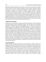
FIGURE 11.10.4
Unit vector geometry for the double-

rod pendulum.
n
n
n
θ

1
1
z
2
2
n
n
n
n
1
1r
2
2r
θ
θ
θ
nnnnn
nnnnn
22112112122
2211211 2122
rr
r
=−
()

+−
()
=+
=−
()
+−
()
=− +
cos sin cos sin
sin cos sin cos
θθ θθ θ θ
θθ θθ θ θ
θ
θθ
F
1
*
F
2
*
T
1
*
T
2
*
F
1
*
F

2
*
T
1
*
T
2
*
Fm m m
G
r
r
11
2
111
22
*
˙˙˙
=− =
()
−
()
annllθθ
θ
Fnn
11
2
11 11 1
2
11 12

22
*
˙
cos
˙˙
sin
˙
sin
˙˙
cos=
()
+
()
+
()
−
()
mmllθθθθ θθθθ
Fa n n n n
21
2
111 2
2
222
2
22
*
˙˙˙ ˙ ˙˙
=− = − +
()

−
()
mm m m m
G
rr
ll l lθθ θ θ
θθ
Fn
n
2111
2
12 22
2
21
111
2
12 22
2
22
22
22
*
˙˙
sin cos
˙˙
sin
˙
cos
˙˙
cos

˙
sin
˙˙
cos
˙
sin
=++
()
+
()
[]
+− + −
()
+
()
[]
m
m
l
l
θθθθθ θθ θ
θθθθθ θθ θ
Tn
1
2
13
12
*
˙˙
=−

()
ml θ
Tn
2
2
23
12
*
˙˙
=−
()
ml θ
0593_C11_fm Page 382 Monday, May 6, 2002 2:59 PM
Generalized Dynamics: Kinematics and Kinetics 383
(11.10.19)
and
(11.10.20)
Finally, from Eq. (11.9.6) the generalized inertia forces are:
(11.10.21)
and
(11.10.22)
Observe how routine the computation is; the principal difficulty is the detail. We will
discuss this later.
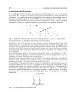
Example 11.10.4: Spring-Supported Particles in a Rotating Tube
Consider again the system of Section 11.7 consisting of a cylindrical tube T containing
three spring-supported particles P
1
, P
2
, and P

3
(or small spheres) as in Figure 11.10.5. As
before, T has mass M and length L and it rotates in a vertical plane with the angle of
rotation being θ as shown. The particles each have mass m, and their positions within T
are defined by the coordinates x
1
, x
2
, and x
3
as in Figure 11.10.6, where ᐉ is the natural
length of each of the springs.
FIGURE 11.10.5
A rotating tube containing spring-supported
particles.
FIGURE 11.10.6
Coordinates of particles within the tube.
vn n n
vn n n
v
vn n n
˙
˙
˙
˙
sin cos
sin cos
sin cos
θ
θ

θ
θ
θ
θ
θ
θθ
θθ
θθ
1
1
1
2
2
1
2
2
22 2
0
22 2
11112
11112
22122
G
G
G
G
=
()
=−
()

+
()
==− +
=
=
()
=−
()
+
()
ll l
ll l
ll l
ωωωωωωωω
˙˙˙˙
,,,
θθθθ
1
1
1
2
2
1
2
2
33
00
BBBB
====nn
F

θ
θθθθ θθθ
1
43 12 12
2
1
2
221
2
2
2
21
*
˙˙ ˙˙
cos
˙
sin=−
()
−
()
−
()
+
()
−
()
mm mll l
F
θ
θθθθ θθθ

2
13 12 12
2
2
2
121
2
1
2
21
*
˙˙ ˙˙
cos
˙
sin=−
()
−
()
−
()
−
()
−
()
mm mll l
P
P
P
n
n

n
T
2
1
3
3
1
2
R

j
i
3ᐉ
2ᐉ
ᐉ
P
P P
n
n
n
T
x
x
x
2
1
3
3
3
1

1
2
2
0593_C11_fm Page 383 Monday, May 6, 2002 2:59 PM
384 Dynamics of Mechanical Systems
The velocities and accelerations of P
1
, P
2
, and P
3
in the fixed or inertial frame R are (see
Eqs. (11.7.2), (11.7.3), and (11.7.4)):
(11.10.23)
(11.10.24)
(11.10.25)
where n
1
, n
2
, and n
3
are the unit vectors shown in Figures 11.10.5 and 11.10.6. Let G be
the mass center of T. Then, from Eq. (11.7.1), the velocity and acceleration of G in R are:
(11.10.26)
Finally, the angular velocity and the angular acceleration of T in R are:
(11.10.27)
As noted in Section 11.7, the system has four degrees of freedom represented by the
coordinates x
1

, x
2
, x
3
, and θ. The corresponding partial velocities and partial angular
velocities are recorded in Eqs. (11.7.5), (11.7.6), and (11.7.7) as:
(11.10.28)
From Eqs. (11.10.23) to (11.10.27), the inertia forces on the particles and the tube may be
represented by:
(11.10.29)
vn na n n
PP
xx xx xx
11
11 1 2 1 1
2
11 12
2=++
()
=−+
()
[]
++
()
+
[]
˙
˙
,
˙˙

˙˙˙˙
˙
lllθθθθ
vn na n n
PP
xx xx xx
22
21 2 2 2 2
2
1222
2222=++
()
=−+
()
[]
++
()
+
[]
˙
˙
,
˙˙
˙˙˙˙
˙
lllθθθθ
vn na n n
PP
xx xx xx
33

31 3 2 3 3
2
1332
3332=++
()
=−+
()
[]
++
()
+
[]
˙
˙
,
˙˙
˙˙˙˙
˙
lllθθθθ
vna nn
GG
LLL=
()
=−
()
+
()
222
2
2

12
˙
,
˙˙˙
θθθ
ωωαα==
˙˙˙
θθnn
33
and
vn v v v n
vvnvv n
vvvnv
˙˙˙˙
˙˙ ˙˙
˙˙˙ ˙
,, ,
,,,
,, ,
x
P
x
P
x
PP
x
P
x
P
x

PP
x
P
x
P
x
PP
x
x
1
1
2
1
3
11
1
2
2
2
3
22
1
3
2
3
3
3
112
122
1

00
002
00
====+
()
====+
()
===
θ
θ
θ
l
l
33
123
123
3
000 2
000
32
2
3
=+
()
====
()
====
l x
L
x

G
x
G
x
GG
xxx
n
vvv vn
n
˙˙˙ ˙
˙˙˙ ˙
,,,
,,,
θ
θ
ωωωωωωωω
Fa n n
Fa n n
Fa
P
P
P
P
P
P
mmxx mx x
mmx x mx x
m
1
1

2
2
3
11
2
1112
22
2
1222
2
222
*
*
*
˙˙
˙˙˙˙
˙
˙˙
˙˙˙˙
˙
=− =− − +
()
[]
−+
()
+
[]
=− =− − +
()
[]

−+
()
+
[]
=−
ll
ll
θθθ
θθθ
33
33
2
1332
2
12
2
3
332
22
12
=− − +
()
[]
−+
()
+
[]
=− =
()
−

()
=− ⋅ − × ⋅
()
=−
()
mx x m x x
MML ML
ML
T
G
TG G
˙˙
˙˙˙˙
˙
˙˙˙
˙˙
*
*
llθθθ
θθ
θ
nn
Fa n n
TI nααωωωωI
0593_C11_fm Page 384 Monday, May 6, 2002 2:59 PM
Generalized Dynamics: Kinematics and Kinetics 385
Finally, from Eq. (11.9.6), the generalized inertia forces are:
(11.10.30)
(11.10.31)
(11.10.32)

or
(11.10.33)
Example 11.10.5: Rolling Circular Disk
As a final example consider again the rolling circular disk D with mass m and radius r of
Figure 11.10.7. (We first considered this system in Section 4.12 and later in Sections 8.13
and 11.3.) As we observed in Section 11.3, this is a nonholonomic system having three
FIGURE 11.10.7
A circular disk rolling on a horizontal
surface.
FvFvFvFvF T
x
x
P
P
x
P
P
x
P
P
x
T
x
T
mx x
1
1
1
1
1

2
2
1
3
3
11
11
2
*
˙
*
˙
*
˙
*
˙
**
˙
*
˙˙
˙
=⋅+⋅+⋅+⋅+⋅
=− − +
()
[]
ω
θl
F vF F vF vF T
x
x

P
P
x
P
P
x
P
P
x
G
T
x
T
v
mx x
2
2
1
1
2
2
2
2
3
3
22
22
2
2
*

˙
*
˙
*
˙
*
˙
*
˙
*
˙˙
˙
=⋅+⋅+⋅+⋅+⋅
=− − +
()
[]
ω
θl
F vF F vF vF T
x
x
P
P
x
P
P
x
P
P
x

G
T
x
T
v
mx x
3
3
1
1
3
2
2
3
3
3
33
33
2
3
*
˙
*
˙
*
˙
*
˙
*
˙

*
˙˙
˙
=⋅+⋅+⋅+⋅+⋅
=− − +
()
[]
ω
θl
F
mx x xm x x x
mx
P
P
P
P
P
P
G
TTθ
θθ θ θθ
ω
θθ θθ
*
˙
*
˙
*
˙
*

˙
*
˙
*
˙
˙˙ ˙
˙
˙˙ ˙
˙
=⋅+⋅+⋅+⋅+⋅
=− +
()
+
()
+
[]
−+
()
+
()
+
[]
−+
(
vF vF vF vF T
1
1
2
2
3

3
11 1 2 2 2
3
222 2
3
ll l l
l
))
+
()
+
[]
−
()
−
()
32 2 12
33
2
2
l x x ML ML
˙˙ ˙
˙
˙˙ ˙˙
θθ θ θ
Fmx x x ML
mxx xx xx
θ
θθ
θ

*
˙˙ ˙˙
˙˙˙
˙
=− +
()
++
()
++
()
[]
−
()
−+
()
++
()
++
()
[]
lll
ll l
1
2
2
2
3
2
2
11 22 33

23 3
223
D
Y
N
Z
N
n
G
c
n
L
N
X
θ
φ
n
3
2
1
1
2
3
ψ
0593_C11_fm Page 385 Monday, May 6, 2002 2:59 PM
386 Dynamics of Mechanical Systems
degrees of freedom. Recall that if we introduce six parameters (say, x, y, z, θ, φ, and ψ) to
define the position and orientation of D we find that the conditions of rolling lead to the
constraint equations (see Eq. (11.3.8), (11.3.9), and (11.3.10)):
(11.10.34)

(11.10.35)
(11.10.36)
where x, y, and z are the Cartesian coordinates of G and θ, φ, and ψ are the orientation
angles of D as in Figure 11.10.7.
The last of these equations is integrable leading to the expression:
(11.10.37)
This expression simply means that D must remain in contact with the surface S. It is
therefore a geometric (or holonomic) constraint. Equations (11.10.34) and (11.10.35), how-
ever, are not integrable in terms of elementary functions. These equations are kinematic
(or nonholonomic) constraints. They ensure that the instantaneous velocity of the contact
point C, relative to S, is zero.
To obtain the generalized inertia forces for this nonholonomic system we may simply
select three of the six parameters as our independent variables. Then the partial velocities
and partial angular velocities may be determined from the coefficients of the derivatives
of these three variables in the expressions for the velocities and angular velocity. That is,
observe that the coordinate derivatives are linearly related in Eqs. (11.10.34), (11.10.35),
and (11.10.36). This means that we can readily solve for the nonselected coordinate deriv-
atives in terms of the selected coordinate derivatives. To illustrate this, suppose we want
to describe the movement of D in terms of the orientation angles θ, φ, and ψ. We may
express the velocity of the mass center G as:
(11.10.38)
where N
1
, N
2
, and N
3
are unit vectors parallel to the X-, Y-, and Z-axes as in Figure 11.10.7.
Then, from Eqs. (11.10.34), (11.10.35), and (11.10.36), we may express v
G

as:
(11.10.39)
˙
˙
sin cos
˙
cos sinxr=+
()
+
[]
ψφ θ φθ θ θ
˙
˙
sin sin
˙
cos cosyr=+
()
−
[]
ψφ θ φθ θ φ
˙
˙
sinzr=− θ θ
zr= cosθ
vNNN
G
xy z=++
˙
˙
˙

123
vN
N
N
G
r
r
r
=+
()
+
[]
++
()
−
[]
−
˙
˙
sin cos
˙
cos sin
˙
˙
sin sin
˙
cos cos
˙
sin
ψφ θ φθ θ φ

ψφ θ φθ θ φ
θθ
1
2
3
0593_C11_fm Page 386 Monday, May 6, 2002 2:59 PM
Generalized Dynamics: Kinematics and Kinetics 387
From Figure 11.10.7, we see that N
1
, N
2
, and N
3
may be expressed in terms of the unit
vectors n
1
, n
2
, and n
3
as:
(11.10.40)
Hence, by substituting into Eq. (11.10.39) v
G
becomes:
(11.10.41)
Also, the angular velocity ωω
ωω
of D relative to S may be expressed as (see Eq. (4.12.2)):
(11.10.42)

Observe that the result of Eq. (11.10.41) could have been obtained directly as ωω
ωω
× rn
3
, the
expression for velocities of points of rolling bodies (see Section 4.11, Eq. (4.11.5)).
The partial velocities of G and the partial angular velocities of D with respect to θ, φ,
and ψ are then:
(11.10.43)
and
(11.10.44)
The inertia force system on D may be represented by a single force F
*
passing through G
together with a couple with torque T
*
where F
*
and T
*
are (see Section 8.13, Eqs. (8.13.7)
to (8.13.12)):
(11.10.45)
and
(11.10.46)
where
(11.10.47)
Nn n n
Nn n n
Nnn

11 1 3
21 2 3
323
=− +
=+ −
=+
cos sin cos sin sin
sin cos cos cos sin
sin cos
φφθθφ
φφθφθ
θθ
vnn
G
rr=+
()
−
˙
˙
sin
˙
ψφ θ θ
12
ωω= + +
()
+
˙
˙
˙
sin

˙
cosθψφθφθnnn
123
vnv nvn
˙˙ ˙
, sin ,
θ
φ
ψ
θ
GG G
rr r=− = =
211
ωωωωωω
˙˙ ˙
, sin cos ,
θ
φ
ψ
θθ==+ =nnnn
1232
Fa nnn
*
=− =− + +
()
mmaaa
G
11 22 33
Tnnn
*

=++TTT
11 22 33
T
T
T
1 1 11 2 3 22 33
2 2 22 3 1 33 11
3 3 33 1 2 11 22
=− + −
()
=− + −
()
=− + −
()
αωω
αωω
αωω
ΙΙΙ
ΙΙΙ
ΙΙΙ
0593_C11_fm Page 387 Monday, May 6, 2002 2:59 PM
388 Dynamics of Mechanical Systems
where a
G
is the acceleration of G relative to the fixed surface S (the inertia frame); where
ω
i
and α
i
(i = 1, 2, 3) are the n

i
components of ωω
ωω
and the angular acceleration αα
αα
of D relative
to S; and, finally, where:
(11.10.48)
From Eqs. (4.12.7) and (4.12.8), a
G
and αα
αα
are:
(11.10.49)
and
(11.10.50)
Hence, F
*
and T
*
may be written as:
(11.10.51)
and
(11.10.52)
Finally, by using Eq. (11.9.6), the generalized inertia forces become:
(11.10.53)
ΙΙ Ι
11 33
2
22

2
42== =mr mr,
an
n
G
rr
r
=+ +
()
+−+ +
()
+− − −
()
˙˙
˙˙
sin
˙
˙
cos
˙˙
˙
˙
cos
˙
sin cos
˙
˙
sin
˙
sin

˙
ψφ θ φθ θ θψφ θφ θ θ
ψφ θ φ θ θ
2
1
2
22 2
3
αα= −
()
++ +
()
+− +
()
˙˙
˙
˙
cos
˙˙
˙˙
sin
˙
˙
cos
˙˙
cos
˙
˙
sin
˙

˙
θψφθ ψφθθφθ
φθφθθψθ
nn
n
12
3
Fn
nn
*
˙˙
˙˙
sin
˙
˙
cos
˙˙
˙
˙
cos
˙
sin cos
˙
˙
sin
˙
sin
˙
=− + +
()

+− +
(
[
+
)
+− − −
()
]
mr ψφ θ φθ θ θψφ θ
φθθ ψφθφ θθ
2
1
2
2
22 2
3
Tn
n
n
*
˙˙
˙
˙
cos
˙
sin cos
˙˙
˙˙
sin
˙

˙
cos
˙˙
cos
˙
˙
=−
()
−−
()
[
++ +
()
++
()
]
mr
22
1
2
3
42
22 2
2
θψφθφ θθ
ψφθθφθ
φθψθ
F
mr
mr

mr
G
θ
θθ
θψθ θφ θ θ
θψφθφ θθ
θψφθφθθ
*
˙
*
˙
*
˙˙
˙
˙
cos
˙
sin cos
˙˙
˙
˙
cos
˙
sin cos
˙˙
˙
˙
cos
˙
sin cos

=⋅+⋅
=−+ +
()
−
()
−−
()
=−
()
+
()
+
()
[]
vF Tωω
22
22
22
42
54 32 54
0593_C11_fm Page 388 Monday, May 6, 2002 2:59 PM
Generalized Dynamics: Kinematics and Kinetics 389
(11.10.54)
and
(11.10.55)
As an aside, we can readily develop the generalized applied (or active) forces for this
system. Indeed, the only applied forces are gravity and contact forces, and of these only
the gravity (or weight) forces contribute to the generalized forces. (The contact forces do
not contribute because they are applied at a point of zero velocity.)
The weight forces may be represented by a single vertical force W passing through G

given by:
(11.10.56)
Then, from Eq. (11.10.43), the generalized forces are:
(11.10.57)
11.11 Potential Energy
In elementary mechanics, potential energy is often defined as the “ability to do work.”
While this is an intuitively satisfying concept it requires further development to be com-
putationally useful. To this end, we will define potential energy to be a scalar function of
the generalized coordinates which when differentiated with respect to one of the coordi-
nates produces the negative of the generalized force for that coordinate. Specifically, we
define potential energy P(q
r
) as the function such that:
(11.11.1)
F
mr
mr
mr
mr
G
φ
φφ
θψ φ θ φθ θ
θψ φ θ θφ θ
θφ θ ψθ
ψθ φ
*
˙
*
˙

*
sin
˙˙
˙˙
sin
˙
˙
cos
sin
˙˙
˙˙
sin
˙
˙
cos
cos
˙˙
cos
˙
˙
˙˙
sin
˙˙
sin
=⋅+⋅
=− + +
()
−
()
++

()
−
()
+
()
=−
()
−
()
vF Tωω
2
2
2
22
2
422 2
42
32 32
θθφθθθ
φθ ψθθ
−
()
[
−
()
+
()
]
52
14 12

2
˙
˙
sin cos
˙˙
cos
˙
˙
cos
Fmr
mr
mr
ψ
ψφ θ φθ θ
ψφθθφθ
ψφθθφθ
*
˙˙
˙˙
sin
˙
˙
cos
˙˙
˙˙
sin
˙
˙
cos
˙˙

˙˙
sin
˙
˙
cos
=− + +
()
−
()
++
()
=−
()
+
()
+
()
[]
2
2
2
2
42 2 2
32 32 52
WN n n=− =− +
()
mg mg
323
sin cosθθ
Fmg F F

xθφ
θ===sin , ,00
Fqrn
rr
=
−∂ ∂ = …
()
D
P 1, ,
0593_C11_fm Page 389 Monday, May 6, 2002 2:59 PM
390 Dynamics of Mechanical Systems
where as before, n is the number of degrees of freedom of the system. (The minus sign is
chosen so that P is positive in the usual physical applications.)
To illustrate the consistency of this definition with the intuitive concept, consider a
particle Q having a mass m in a gravitational field. Let Q be at an elevation h above a
fixed level surface S as in Figure 11.11.1. Then, if Q is released from rest in this position,
the work w done by gravity as Q falls to S is:
(11.11.2)
From a different perspective, if h is viewed as a generalized coordinate, the velocity v
of Q and, consequently, the partial velocity v
h
of Q (relative to h) are:
(11.11.3)
where k is the vertical unit vector as in Figure 11.11.1. The generalized force due to gravity
is then:
(11.11.4)
Let P be a potential energy defined as:
(11.11.5)
Then, from Eq. (11.11.1), F
h

is:
(11.11.6)
which is consistent with the results of Eq. (11.11.4).
As a second illustration, consider a linear spring as in Figure 11.11.2. Let the spring have
modulus k and natural length ᐉ. Let the spring be supported at one end, O, and let its
other end, Q, be subjected to a force with magnitude F producing a displacement x of Q,
as depicted in Figure 11.11.2. The movement of Q has one degree of freedom represented
by the parameter x. The velocity v and partial velocity of Q are then:
(11.11.7)
FIGURE 11.11.1
A particle Q above a level surface S.
FIGURE 11.11.2
A force applied to a linear spring.
w mgh=
vk k==
˙
hv
h
and
Fmg mg
hh
=− ⋅ =−kv
P ==w mgh
Fhmg
h
=−∂ ∂ =−P
v
˙
x
vn vn==

˙
˙
x
x
and
k
h
Q(m)
S
n
k
Q
F
x
ᐉ
O
0593_C11_fm Page 390 Monday, May 6, 2002 2:59 PM
Generalized Dynamics: Kinematics and Kinetics 391
The force S exerted on Q by the spring is:
(11.11.8)
The generalized force F
x
relative to x is then:
(11.11.9)
Let a potential energy function P be defined as:
(11.11.10)
Then, from Eq. (11.11.1), we have:
(11.11.11)
which is consistent with Eq. (11.11.9).
It happens that Eqs. (11.11.5) and (11.11.10) are potential energy functions for gravity

and spring forces in general. Consider first Eq. (11.11.5) for gravity forces. Suppose Q is
a particle with mass m. Let Q be a part of a mechanical system S having n degrees of
freedom represented by the coordinates q
r
(r = 1,…, n). Recall from Eq. (11.6.5) that the
contribution of the weight force on Q to the generalized force F
r
for the coordinate q
r
is:
(11.11.12)
where h is the elevation of Q above a reference level as in Figure 11.11.3.
From Eq. (11.11.2), if a potential energy function P is given by mgh, Eq. (11.11.1) gives
the contribution to the generalized force of q
r
for the weight force as:
(11.11.13)
which is consistent with Eq. (11.11.12).
Consider next Eq. (11.11.10) for spring forces. Suppose Q is a point at the end of a spring
which is part of a mechanical system S as depicted in Figure 11.11.4. Let S have n degrees
FIGURE 11.11.3
Elevation of a particle Q of a mechanical system S.
FIGURE 11.11.4
A spring within a mechanical system S.
Sn n=− =−Fkx
Fkx
x
x
=⋅ =−Sv
˙

P =
()
12
2
kx
−∂ ∂ =− =P xkxF
x
ˆ
F
r
ˆ
Fmghq
rr
=− ∂ ∂
ˆ
F
r
ˆ
Fqmghq
rr r
=−∂ ∂ =− ∂ ∂P
Q(m)
r
h(q ,t)
R
S
k
R
O
Q

n
S
0593_C11_fm Page 391 Monday, May 6, 2002 2:59 PM
392 Dynamics of Mechanical Systems
of freedom represented by the coordinates q
r
(r = 1,…, n). Then, from Eq. (11.6.7), we
recall that the contribution of the spring force to the generalized force on S, for the
coordinate q
r
, is:
(11.11.14)
where f(x) is the magnitude of the spring force due to a spring extension, or compression,
x. For a linear spring f(x) is simply kx; hence, for a linear spring, is:
(11.11.15)
From Eq. (11.11.10), if we let the potential energy function P be (1/2)kx
2
, we obtain from
Eq. (11.11.1) as:
(11.11.16)
which is consistent with Eq. (11.11.15).
Alternatively, for a nonlinear spring, we may let the potential energy function have the
form:
(11.11.17)
Then, from Eq. (11.11.1), becomes
(11.11.18)
which is consistent with Eq. (11.11.14).
The definition of Eq. (11.11.1) and these simple examples show that if a potential energy
function is known we can readily obtain the generalized applied (or active) forces. Indeed,
the examples demonstrate the utility of potential energy for finding generalized forces.

Moreover, for gravity and spring forces, Eqs. (11.11.5), (11.11.10), and (11.11.17) provide
expressions for potential energy functions. This, however, raises a question about other
forces; that is, what are the potential energy functions for forces other than gravitational
or spring forces? The answer is found by considering again Eq. (11.11.1): If
(11.11.19)
Unfortunately, it is not always possible to perform the integration indicated in Eq.
(11.11.19). Indeed, the integral represents an anti-partial differentiation with respect to
ˆ
F
r
ˆ
Ffx
x
q
r
r
=−
()
∂
∂
ˆ
F
r
ˆ
Fkx
x
q
r
r
=−

∂
∂
ˆ
F
r
ˆ
Fq
q
kx kx
x
q
rr
rr
=−∂ ∂ =−
∂
∂
()
[]
=−
∂
∂
P 12
2
P =
()
∫
fd
x
0
ξξ

ˆ
F
r
ˆ
FP
rr
r
x
r
q
q
fd fx
x
q
=−∂ ∂ =
∂
∂
()








=−
()
∂
∂

∫
0
ξξ
∂
∂
=− =−
∫
x
q
Fdq
r
rrr
FP then
0593_C11_fm Page 392 Monday, May 6, 2002 2:59 PM
Generalized Dynamics: Kinematics and Kinetics 393
each of the q
r
. Also, if the F
r
involve derivatives of the (such as with “dissipation forces”),
the integrals will not exist, because P is to depend only on the q
r
.
Further, observe that if knowledge of the generalized forces is needed to obtain a
potential energy function which in turn is to be used to obtain the generalized forces, little
progress has been made. Therefore, in the solution of practical problems as in machine
dynamics, potential energy is useful primarily for gravity and spring forces. Finally, it
should be noted that potential energy is not a unique function. Indeed, from Eq. (11.11.1),
we see that the addition of a constant to any valid potential energy function P also produces
a valid potential energy function.

It may be helpful to consider another illustration. Consider again the system of the
rotating tube containing three spring-supported particles as in Figures 11.11.5 and 11.11.6.
We discussed this system in Section 11.7, and we will use the same notation here without
repeating the description (see Section 11.7 for the details).
Recall from Eqs. (11.7.14) to (11.7.17) that the generalized forces for the coordinates x
1
,
x
2
, x
3
, and θ are:
(11.11.20)
(11.11.21)
(11.11.22)
(11.11.23)
FIGURE 11.11.5
A rotating tube containing spring-
connected particles.
FIGURE 11.11.6
Coordinates of the particles within
the tube.
˙
q
r
F
x
mg kx kx
1
21

2=+−cosθ
F
x
mg kx kx kx
2
31 2
2=++−cosθ
F
x
mg kx kx
3
2
32
=−+cosθ
F
θ
θθ=−
()
−+++
()
Mg L mg x x x26
123
sin sinl
0593_C11_fm Page 393 Monday, May 6, 2002 2:59 PM
394 Dynamics of Mechanical Systems
In the development of these generalized forces we discovered that the only forces
contributing to these forces were gravity and spring forces. The contact forces between
the smooth tube and the particles did not contribute to the generalized forces; hence, we
should be able to form a potential energy function for the system. To this end, using Eqs.
(11.11.5) and (11.11.10) we obtain the potential energy function:

(11.11.24)
where the reference level for the gravitational forces is taken through the support pin O.
From Eq. (11.11.1) we can immediately determine the generalized forces. That is,
(11.11.25)
By substituting from Eq. (11.11.24) into (11.11.25), we obtain results identical to those of
Eqs. (11.11.20) to (11.11.23).
11.12 Use of Kinetic Energy to Obtain Generalized Inertia Forces
Just as potential energy can be used to obtain generalized applied (active) forces, kinetic
energy can be used to obtain generalized inertia (passive) forces. In each case, the forces
are obtained through differentiation of the energy functions. In this section, we will
establish the procedures for using kinetic energy to obtain the generalized inertia forces.
To begin the analysis, recall Eq. (11.4.7) concerning the projection of the acceleration of
a particle on the partial velocity vectors:
(11.12.1)
This expression, which is valid only for holonomic systems (see Section 11.3), provides a
means for relating the generalized inertia forces and kinetic energy. To this end, let P be
a particle with mass m of a holonomic mechanical system S having n degrees of freedom
represented by the coordinates q
r
(r = 1,…, n). Then, the inertia force F
*
on P is:
(11.12.2)
where a is the acceleration of P in an inertial reference frame R. Recall further that the
kinetic energy K of P is:
(11.12.3)
P =− +
()
−+
()

−+
()
−
()
+
()
+
()
−
()
+
()
−
()
mg x mg x mg x
Mg L kx k x x k x x
lll
123
1
2
21
2
32
2
23
21212 12
cos cos cos
cos
θθθ
θ

FPFP PFP
xx x
xxFx
12 3
123
=−∂ ∂ =−∂ ∂ =−∂ ∂ =−∂ ∂,,,
θ
θ
av
vv
⋅=
∂
∂






−
∂
∂






˙
q

rr
r
d
dt q q
1
2
1
2
22
Fa
*
=−m
K =
1
2
2
v
0593_C11_fm Page 394 Monday, May 6, 2002 2:59 PM
Generalized Dynamics: Kinematics and Kinetics 395
By multiplying Eq. (11.12.1) by the mass m of P, we have:
(11.12.4)
or by using Eqs. (11.12.2) and (11.12.3) we have:
(11.12.5)
Consider next a set of particles P
i
(i = 1,…, N) as parts of a mechanical system S having
n degrees of freedom. Then, by superposing (or adding together) equations as Eq. (11.12.5)
for each of the particles, we obtain an expression identical in form to Eq. (11.12.5) and valid
for the set of particles. Finally, if the set of particles is a rigid body, Eq. (11.12.5) also holds.
To illustrate the use of Eq. (11.12.5), consider again the elementary examples of the

foregoing section.
Example 11.12.1: Simple Pendulum
Consider first the simple pendulum as in Figure 11.12.1, where we are using the same
notation as before. Recall that this system has one degree of freedom represented by the
angle and that the velocity and partial velocity of the bob P are (see Eqs. (11.10.1) and
(11.10.4)):
(11.12.6)
The kinetic energy of P is then:
(11.12.7)
Then, by using Eq. (11.12.5), the generalized inertia force is:
(11.12.8)
This result is identical with that of Eq. (11.10.5).
FIGURE 11.12.1
The simple pendulum.
m
d
dt q
m
q
q
rr
r
av v v⋅=
∂
∂











−
∂
∂




˙
˙
1
2
1
2
22
F
q
rr
r
d
dt
K
q
K
q
*

˙
=−
∂
∂






+
∂
∂
vn vn
PP
==ll
˙
˙
θ
θ
θ
θ
and
Km m
P
=
()
=
()
1

2
12
2
22
v l
˙
θ
F
θ
*
F
θ
θ
θ
θ
θθ
*
˙˙˙
=−
∂
∂











+
∂
∂




=−
d
dt
mmm
1
2
1
2
22 22 2
lll
θ
ᐉ
R
O
P
n
n

r
θ
0593_C11_fm Page 395 Monday, May 6, 2002 2:59 PM
396 Dynamics of Mechanical Systems

Example 11.12.2: Rod Pendulum
Consider next the rod pendulum of Figure 11.12.2, using the same notation as before.
Recall that the mass center velocity v
G
and the angular velocity of the rod are (see Eqs.
(11.10.6) and (11.10.7)):
(11.12.9)
Hence, the kinetic energy K of the rod is:
(11.12.10)
Then, from Eq. (11.12.5), the generalized inertia force is:
(11.12.11)
This result is the same as in Eq. (11.10.11).
Example 11.12.3: Double-Rod Pendulum
To extend this last example, consider again the double-rod pendulum of Figure 11.12.3.
Unlike the two above examples, this system has two degrees of freedom, as represented
by the angles θ
1
and θ
2
.
FIGURE 11.12.2
The rod pendulum.
FIGURE 11.12.3
A double-rod pendulum.
vn n
Gz
=
()
=l 2
˙˙

θθ
θ
and ωω
Km
mm
m
GG
=
()
+
()
=
()()
+
()( )
=
()
12 12
12 2 12 112
16
22
2
222
22
vIωω
ll
l
˙˙
˙
θθ

θ
F
θ
*
F
θ
θ
*
˙˙
=−
()
13
2
ml
O
θ
B

G
G
B
1
2
1
1
2
2
Q
θ
0593_C11_fm Page 396 Monday, May 6, 2002 2:59 PM

Generalized Dynamics: Kinematics and Kinetics 397
In our earlier analysis of this system we found that the mass center velocities and the
angular velocities of the rods were (see Eqs. (11.10.12)):
(11.12.12)
where, as before, the unit vectors are as shown in Figure 11.12.4.
The kinetic energy of the system is then:
(11.12.13)
Then, from Eq. (11.12.5), the generalized inertia forces and are:
(11.12.14)
and
(11.12.15)
These results are identical with the Eqs. (11.10.21) and (11.10.22).
FIGURE 11.12.4
Unit vector geometry for the double-
rod pendulum.
θ

n
n
n
n
n
n
n
1
1r
2θ
2r
3
2

1
θ
vnvnn
nn
GG
BB
12
12
22
11 11 22
13 23
=
()
=+
()
==
lll
˙
,
˙˙
˙
,
˙
θθθ
θθ
θθθ
ωωωω
Kv
v
=

()
()
+
()
()
+
()
()
+
()
()
=
()
()
+
()( )
+
()
+−
()
+
12 12
12 12
12 4 12 112
12
1
1
1
2
2

2
22
22
2
1
22
1
2
2
1
22
12 2 1
2
m
m
mm
m
G
G
B
G
G
B
I
I
ωω
ωω
lll
ll l
˙˙

˙˙˙
cos
θθ
θθθθθ
44
12 112
23 12
16
2
2
2
2
2
2
1
22
12 2 1
2
2
2
()
[
+
()( )
=
()
+
()
−
()

+
()
˙
˙
˙˙˙
cos
˙
θ
θ
θθθθθ
θ
mm
mm
m
l
ll
l
F
θ
1
*
F
θ
2
*
F
θ
θθθθ θθθ
1
43 12 12

2
1
2
221
2
2
2
21
*
˙˙ ˙˙
cos
˙
sin=−
()
−
()
−
()
+
()
−
()
mm mll l
F
θ
θθθθθθθ
2
13 12 12
2
2

2
121
2
1
2
21
*
˙˙ ˙˙
cos
˙
sin=−
()
−
()
−
()
−
()
−
()
mm mll l
0593_C11_fm Page 397 Monday, May 6, 2002 2:59 PM
398 Dynamics of Mechanical Systems
Example 11.12.4: Spring-Supported Particles in a Rotating Tube
For another example illustrating the use of kinetic energy to obtain generalized inertia
forces, consider again the system of spring-supported particles in a rotating tube as in
Figure 11.12.5. (We considered this system in Sections 11.7 and 11.11.) Recall that this
system has four degrees of freedom represented by the coordinates x
1
, x

2
, x
3
, and θ, as
shown in Figures 11.12.5 and 11.12.6.
The velocities of the particles, the tube mass center velocity, and the angular velocity of
the tube in the inertia frame R are (see Eqs. (11.10.23) through (11.10.27)):
(11.12.16)
where the notation is the same as we used in Section 11.7 and 11.11.
The kinetic energy of the system is then:
(11.12.17)
FIGURE 11.12.5
Rotating tube containing spring-supported
particles.
FIGURE 11.12.6
Coordinates of particles in the tube.
P
P
P
n
n
n
T
2
1
3
3
1
2
R

θ
j
i
O
3ᐉ
2ᐉ
ᐉ
P
P P
n
n
n
T
x
x
x
2
1
3
3
3
1
1
2
2
vn n
vn n
vn n
vn
n

P
P
P
G
xx
xx
xx
L
1
2
3
11 1 2
21 2 2
31 3 3
2
3
2
3
2
=++
()
=++
()
=++
()
=
()
=
˙
˙

˙
˙
˙
˙
˙
˙
l
l
l
θ
θ
θ
θ
θωω
Kv v v
v
=
()
+
()
+
()
+
()
+
()
=
()
++
()

++ +
()
+
[
++
()
]
+
()( )
1
2
1
2
1
2
1
2
1
2
12 2
3122
12
3
22
2
2
2
1
2
1

2
2
2
2
2
2
2
3
2
3
2
2
2
mmm
M
mx x x x x
xML
PP
P
G
I ωω
˙
˙
˙
˙
˙
˙˙
ll
l
θθ

θ
θθθ
222
12 112+
()( )
ML
˙
0593_C11_fm Page 398 Monday, May 6, 2002 2:59 PM
Generalized Dynamics: Kinematics and Kinetics 399
Using Eq. (11.12.5), the generalized inertia forces are then:
(11.12.18)
(11.12.19)
(11.12.20)
(11.12.21)
These results are the same as those of Eqs. (11.10.30) to (11.10.33).
Example 11.12.5: Rolling Circular Disk
For an example where Eq. (11.12.5) cannot be used to determine generalized inertia forces,
consider again the nonholonomic system consisting of the rolling circular disk on the flat
horizontal surface as shown in Figure 11.12.7. (Recall that Eq. (11.12.5) was developed for
holonomic systems [that is, systems with integrable or nonkinematic constraint equations]
and, as such, it is not applicable for nonholonomic systems [that is, systems with kinematic
or nonintegrable constraint equations].)
Due to the rolling constraint, the disk has three degrees of freedom instead of six, as would
be the case if the disk were unrestrained. Recall from Eqs. (11.10.34), (11.10.35), and (11.10.36)
that the condition of rolling (zero contact point velocity) produces the constraint equations:
(11.12.22)
(11.12.23)
(11.12.24)
FIGURE 11.12.7
Circular disk rolling on a horizontal surface S.

F
x
mx m x
1
11
2*
˙˙
˙
=− + +
()
l θ
F
x
mx m x
2
22
2
2
*
˙˙
˙
=− + +
()
l θ
F
x
mx m x
3
33
2

3
*
˙˙
˙
=− + +
()
l θ
F
θ
θ
θ
θ
*
˙˙
˙˙˙
˙
˙˙
=− +
()
++
()
++
()
[]
−+
()
++
()
++
()

[]
−
()
mx x x
mxx xx xx
ML
lll
ll l
1
2
2
2
3
2
11 22 33
2
23
223
3
˙
˙
˙
sin cos
˙
cos sinxr=+
()
+
[]
ψφ θ φθ θ φ
˙

˙
˙
sin sin
˙
cos cosyr=+
()
−
[]
ψφ θ φθ θ φ
˙
˙
sinzr=− θ θ
0593_C11_fm Page 399 Monday, May 6, 2002 2:59 PM
400 Dynamics of Mechanical Systems
The first two of these equations are nonintegrable in terms of elementary functions;
therefore, the system is nonholonomic.
With three constraint equations, the disk has three degrees of freedom. These may
conveniently be represented by the angles θ, φ, and ψ, and in terms of these angles the
mass center velocity and the disk angular velocity are (see Eqs. (11.10.41) and (11.10.42)):
(11.12.25)
and
(11.12.26)
Hence, the kinetic energy of the disk is:
(11.12.27)
where the moments of inertia I
11
, I
22
, and I
33

are:
(11.12.28)
Assuming (erroneously) that Eq. (11.12.5) can be used to determine the generalized
inertia forces, we have:
(11.12.29)
(11.12.30)
(11.12.31)
In Section 11.10, in Eqs. (11.10.53), (11.10.54), and (11.10.55), we found , , and to be:
(11.12.32)
vnn
G
rr=+
()
−
˙
˙
sin
˙
ψφ θ θ
12
ωω= + +
()
+
˙
˙
˙
sin
˙
cosθψφθφθnnn
123

Km
mr r
G
=
()
()
+⋅⋅
=+
()
+






+++
()
+
()






12
1
2
1

2
1
2
2
2
2
22
11
2
22
2
33
2
vIωωωω
˙
˙
sin
˙
˙
˙
˙
sin
˙
cos
ψφ θ θ
θψφθ φθII I
II I
11 33
2
22

2
42== =mr mr,
F
θ
θ
θ
θψφθφθθ
*
˙
˙˙
˙
˙
cos
˙
sin cos
=−
∂
∂






+
∂
∂
=−
()
−

()
−
()
[]
d
dt
KK
mr
22
54 32 54
F
θ
ψθ φ θ φ θ
ψθ θ θφ θ θ
*
˙˙
sin
˙˙
sin
˙˙
cos
˙
˙
cos
˙
˙
sin cos
=−
()
+

()
+
()
[
+
()
+
()
]
mr
222
32 32 14
3 2 11 4
F
ψ
ψφ θφθ θ
*
˙˙
˙˙
sin
˙
˙
cos=−
()
[
++
()
mr
2
32

F
θ
*
F
φ
*
F
ψ
*
F
θ
θψφθφθθ
*
˙˙
˙
˙
cos
˙
sin cos=−
()
−
()
−
()
[]
mr
22
54 32 54
0593_C11_fm Page 400 Monday, May 6, 2002 2:59 PM
Generalized Dynamics: Kinematics and Kinetics 401

(11.12.33)
and
(11.12.34)
While Eqs. (11.12.29), (11.12.30), and (11.12.31) are similar to Eqs. (11.12.32), (11.12.33),
and (11.12.34), they are not identical; therefore, Eq. (11.12.5) is not valid for nonholonomic
systems. It happens, however, that Eq. (11.12.5) may be modified and expanded to also
accommodate nonholonomic systems. Although the details of this expansion are beyond
the scope of this text, the interested reader is referred to References 11.2 and 11.4.
11.13 Closure
Our objective in this chapter has been to introduce the principles and procedures of
generalized dynamics. Our intention was to obtain a working knowledge of the elementary
procedures. More advanced procedures, such as those applicable with large multibody
systems and, to some extent, those concerned with nonholonomically constrained systems,
have not been discussed because they are beyond our scope at this time. The interested
reader may want to refer to References 11.2 and 11.4 and later chapters for a discussion
of these topics.
The examples are intended to demonstrate the principal advantages of the generalized
procedures over the procedures used in elementary mechanics, including: (1) non-working
constraint forces do not contribute to the generalized forces so these forces may be simply
ignored in the analysis; and (2) for holonomic systems (which include the vast majority
of systems of interest in machine dynamics), generalized inertia forces may be computed
from kinetic energy functions. This in turn means that vector acceleration need not be
computed, thus saving considerable analysis effort.
In addition to these advantages, if a system possesses a potential energy function, the
generalized active (or applied) forces may be obtained by a single derivative of the
potential energy function. Moreover, for gravity and spring forces (which are prevalent
in machine dynamics), the potential energy functions may often be directly obtained from
Eqs. (11.11.5) and (11.11.10). In the next chapter, we will consider the application of these
procedures in obtaining equations of motion.
References

11.1. Kane, T. R., Dynamics, Holt, Rinehart & Winston, New York, 1968, p. 78.
11.2. Kane, T. R., and Levinson, D. A., Dynamics: Theory and Applications, McGraw-Hill, New York,
1985, p. 100.
F
φ
ψθ φ θ φθθθ
φθ ψθθ
*
˙˙
sin
˙˙
sin
˙
˙
sin cos
˙˙
cos
˙
˙
cos
=−
()
[
+
()
+
()
+
()
−

()
]
mr
22
32 32 52
14 12
F
ψ
ψφθθφθ
*
˙˙
˙˙
sin
˙
˙
cos=−
()
+
()
+
()
[]
mr
2
32 32 52
0593_C11_fm Page 401 Monday, May 6, 2002 2:59 PM
402 Dynamics of Mechanical Systems
11.3. Kane, T. R., Analytical Elements of Mechanics, Vol. 1, Academic Press, New York, 1959, p. 128.
11.4. Huston, R. L., and Passerello, C. E., Another look at nonholonomic systems, J. Appl. Mech., 40,
101–104, 1973.

11.5. Huston, R. L., Multibody Dynamics, Butterworth-Heinemann, Stoneham, MA, 1990.
11.6 Huston, R. L., and Liu, C. Q., Formulas for Dynamic Analysis, Marcel Dekker, New York, 2001.
Problems
Section 11.2 Coordinates, Constraints, and Degrees of Freedom
P11.2.1: Determine the number of degrees of freedom of the following systems:
a. Pair of eyeglasses
b. Pair of pliers or pair of scissors
c. Child’s tricycle rolling on a flat horizontal surface (let the tricycle be modeled
by a frame, two rear wheels, and a front steering wheel)
d. Human arm model consisting of three rigid bodies representing the upper arm,
the lower arm, and the hand (with spherical joints at the wrist and shoulder and
a hinge joint at the elbow)
e. Pencil writing on a sheet of paper
f. Eraser, erasing a chalk board
P11.2.2: An insect A is crawling on the surface of a sphere B with radius r as represented
in Figure P11.2.2. Let the coordinates of A relative to a Cartesian X, Y, Z system with origin
O at the center of the sphere be (x, y, z). What are the constraints and degrees of freedom?
P11.2.3: A knife blade B is being held such that its cutting edge E remains horizontal
(Figure P11.2.3). Let B be used to cut a soft medium such as a soft cheese. Let the cheese
restrict B so that B has no velocity perpendicular to its plane. How many degrees of
freedom does B have? What are the constraint equations?
FIGURE P11.2.2
An insect crawling on a sphere.
FIGURE P11.2.3
A knife blade cutting a soft medium.
0593_C11_fm Page 402 Monday, May 6, 2002 2:59 PM
Generalized Dynamics: Kinematics and Kinetics 403
Section 11.4 Vector Functions, Partial Velocity, and Partial Angular Velocity
P11.4.1: Consider again the double-rod pendulum of Figure 11.4.3 and as shown again in
Figure P11.4.1. As before, let each rod be identical with length

ᐉ. Let the rod orientations
be defined by the “relative” orientation angles β
1
and β
2
as in Figure P11.4.1. Find the
velocities of mass centers G
1
and G
2
, and the angular velocities of B
1
and B
2
. Find the
partial velocities of G
1
and G
2
for β
1
and β
2
and the partial angular velocities of B
1
and B
2
for β
1
and β

2
. Compare the results with those of Eqs. (11.4.23) and (11.4.24).
P11.4.2: A rotating rod B has two collars C
1
and C
2
which can slide relative to B as indicated
in Figure P11.4.2. Let the orientation of B be and let x
1
locate C
1
relative to the pin O and let
x
2
locate C
2
relative to C
1
. Find the partial velocities of C
1
and C
2
with respect to θ, x
1
, and x
2
.
P11.4.3: A box B moving in a reference frame R is oriented in R by dextral (Bryan)
orientation angles and defined as follows: let unit vectors n
x

, n
y
, and n
z
fixed in B be
aligned with unit vectors N
X
, N
Y
, and N
Z
, respectively, fixed in R as depicted in Figure
P11.4.3. Then, let B be successively rotated in R about axes parallel to n
x
, n
y
, and n
z
through
angles α, β, and γ, bringing B into a general orientation in R. Show that the angular velocity
of B in R may then be expressed as:
where s and c are abbreviations for sine and cosine (see Section 4.7).
FIGURE P11.4.1
A double-rod pendulum with relative
orientation angles.
FIGURE P11.4.2
A rotating rod with sliding collars.
FIGURE P11.4.3
A box B moving in a reference frame R.
G

G
n
n
n
B
B
1
1
1
1
2
2
2
2
β

3
β
B
C
C
θ
x
x
1
1
2
2
N
X

N
N
B
n
n
n
z
x
y
Z
Y
X
R
Y
Z
RB
xy
z
cc s c cs
s
ωω= +
()
+−
()
++
()
˙
˙˙
˙
˙

˙
αβ βα
αγ
β
γγ γ
β
γ
β
nn
n
0593_C11_fm Page 403 Monday, May 6, 2002 2:59 PM
404 Dynamics of Mechanical Systems
P11.4.4: See Problem P11.4.3. Express
R
ωω
ωω
B
in terms of the unit vectors N
X
, N
Y
, and N
Z
.
P11.4.5: See Problems 11.4.3 and P11.4.4. Find the partial angular velocities of B in R for
α, β, and γ. (Express the results in terms of both n
x
, n
y
, and n

z
and N
X
, N
Y
, and N
Z
.
P11.4.6: See Problems P11.4.3, P11.4.4, and P11.4.5. Let O be the origin of a Cartesian axis
system X, Y, Z fixed in R, and let Q be a vertex of B as in Figure P11.4.6. Let the velocity
of Q in R be expressed alternatively as:
and
a. Express , , and in terms of , , and .
b. Express , , and in terms of , , and .
P11.4.7: See Problem P11.4.6. Find the partial velocities of Q in R for the coordinates x, y,
z, X, Y, and Z. Express the results in terms of both n
x
, n
y
, and n
z
and N
X
, N
Y
, and N
Z
.
P11.4.8: See Problem 11.4.6. Let the sides of the box B have lengths a, b, and c, as represented
in Figure P11.4.6, and let P be a vertex of B as shown. Find the velocity of P in R. Express

the results in terms of both n
x
, n
y
, and n
z
and N
X
, N
Y
, and N
Z
. Use either , , and or
, , and for convenience.
P11.4.9: See Problems P11.4.3 to P11.4.8. Find the partial velocities of P in R for the
coordinates x, y, z, X, Y, Z, α, β, and γ. Express the results in terms of both n
x
, n
y
, and n
z
and N
X
, N
Y
, and N
Z
.
Section 11.5 Generalized Forces: Applied (Active) Forces
P11.5.1: A simple pendulum with length ᐉ of 0.5 m and bob P mass of 2 kg is subjected

to a constant horizontal force F of 5 N as represented in Figure P11.5.1. Determine the
generalized active force F
θ
on P for the orientation angle θ. (Include the contributions of
F, gravity, and the cable tension.)
FIGURE P11.4.6
A box B moving in a reference frame R.
RQ
XYZ
XYZVNNN=++
˙
˙
˙
RQ
xyz
xyzVnnn=++
˙
˙
˙
˙
x
˙
y
˙
z
˙
X
˙
Y
˙

Z
˙
X
˙
Y
˙
Z
˙
x
˙
y
˙
z
O
N
X
N
N
c
a
b
P
B
n
n
n
Q
z
x
y

Z
Y
X
˙
x
˙
y
˙
z
˙
X
˙
Y
˙
Z
0593_C11_fm Page 404 Monday, May 6, 2002 2:59 PM
Generalized Dynamics: Kinematics and Kinetics 405
P11.5.2: Repeat Problem P11.5.1 for a force F given as follows:
a. F = 4n
y
N
b. F = 3n
x
+ 4n
y
N
c. F = 5n
r
N
d. F = 5n

θ
N
P11.5.3: A double-rod pendulum consists of two identical pin-connected rods each having
mass m and length ᐉ as depicted in Figure P11.5.3. Let there be a particle P with mass M
at the end of the lower rod. Assuming the pin connections are frictionless, find the
generalized active forces for the orientation angles θ
1
and θ
2
shown in Figure P11.5.3.
P11.5.4: Repeat Problem P11.5.3 for the “relative” orientation angles β
1
and β
2
shown in
Figure P11.5.4.
P11.5.5: See Problem P11.5.3. A triple-rod pendulum consists of three pin-connected rods
each having mass m and length ᐉ as depicted in Figure P11.5.5. Let there be a particle P
with mass M at the end of the lower rod. Assuming the pin connections are frictionless,
find the generalized active forces for the orientation angles θ
1
, θ
2
, and θ
3
shown in Figure
P11.5.3.
FIGURE P11.5.1
A simple pendulum subjected to a
horizontal force.

FIGURE P11.5.3
A double-rod pendulum with a concentrated
end mass.
FIGURE P11.5.4
A double-rod pendulum with a concentrated end
mass and relative orientation angles.
θ
n
n

r
F
| F | = 5N
P(2 kg)
ᐉ = 0.5 m
n
n
y
x
θ
θ

1
2
ᐉ

P(M)
ᐉ
θ
1

2
β
ᐉ

P(M)
ᐉ
β
0593_C11_fm Page 405 Monday, May 6, 2002 2:59 PM
406 Dynamics of Mechanical Systems
P11.5.6: Repeat Problem P11.5.5 for the relative orientation angles β
1
, β
2
, and β
3
shown in
Figure P11.5.6.
P11.5.7: See Problem P11.5.5. Let there be linear torsion springs at the pin joints of the
triple-rod pendulum. Let these springs have moduli k
1
, k
2
, and k
3
, and let the resulting
moments generated by the springs be parallel to the pin axes and proportional to the
relative angles β
1
, β
2

, and β
3
between the rods as shown in Figure P11.5.6. Find the
contribution of the spring moments to the generalized active forces for the angles θ
1
, θ
2
,
and θ
3
.
P11.5.8: Repeat Problem P11.5.7 for the relative orientation angles β
1
, β
2
, and β
3
.
P11.5.9: An elongated box kite K, depicted in Figure P11.5.9A, is suddenly subjected to
turbulent wind gusts creating forces on K as represented in Figure P11.5.9B. Let the wind
forces be modeled by forces F
1
, F
2
,…, F
8
, whose directions are shown in Figure P11.5.9B
and whose magnitudes are:
Let the orientation of K be defined by dextral orientation angles α, β, and γ, and let the
angular velocity ωω

ωω
of K be expressed as (see Problem P11.4.3):
where n
1
, n
2
, and n
3
are unit vectors parallel to the edges of K as shown in Figure P11.5.9B.
Finally, let the velocity v of the tether attachment point O of K be:
Find the generalized forces F
α
, F
β
, and F
γ
due to the wind forces F
1
, F
2
,…, F
8
.
P11.5.10: Repeat Problem P11.5.9 by first replacing F
1
, F
2
,…, F
8
by a single force F passing

through O together with a couple with torque T; then, use Eq. (11.5.7) to determine F
α
,
F
β
, and F
γ
.
FIGURE P11.5.5
A triple-rod pendulum with a concentrated end
mass.
FIGURE P11.5.6
A triple-rod pendulum with concentrated end mass
and relative orientation angles.
θ

1
2

3
ᐉ


P(M)
θ
θ
ᐉ
ᐉ
1
2

3
ᐉ


P(M)
β


β
β
ᐉ
ᐉ
FF F F
FF F F
12 3 4
56 7 8
56 6 7
810138
== = =
== = =
lb, lb, lb, lb,
lb, lb, lb, lb
ωω= +
()
+−
()
++
()
˙
˙˙

˙˙
˙
αβ βα αγ
β
γγ γ
β
γ
β
cc s c cs snnn
123
vn n n=−+325
123
ft sec
0593_C11_fm Page 406 Monday, May 6, 2002 2:59 PM