Dynamics of Mechanical Systems 2009 Part 12 pptx

532 Dynamics of Mechanical Systems
Here we see that both the resultant primary and secondary inertia forces are also
balanced, leaving the only unbalance with the resultant primary moments. Thus, we have
still further improvement in the balance.
These examples demonstrate the wide range of possibilities available to the engine
designer; however, the examples are not meant to be exhaustive. Many other practical
configurations are possible. The examples simply show that the crankshaft configuration
can have a significant effect upon the engine balance. In the following section, we will
extend these concepts and analyses to eight-cylinder engines.
15.10 Eight-Cylinder Engines: The Straight-Eight and the V-8
If we consider engines with eight cylinders the number of options for balancing increases
dramatically. The analysis procedure, however, is the same as in the foregoing section. To
illustrate the balancing procedure, consider an engine with eight cylinders in a line (the
straight-eight engine) and with crank angles φ
i
for the connecting rods arranged incremen-
tally at 90° along the shaft. Table 15.10.1 provides the listing of the φ
i
for the eight cylinders
(i = 1,…, 8) together with the trigonometric functions needed to test for balancing. A glance
at the table immediately shows that the engine with this incremental 90° crank angle
sequence has a moment unbalance.
This raises the question as to whether there are crank angle configurations where com-
plete balancing would occur, within the approximations of our analysis. To respond to this
question, consider again the four-cylinder engine of the previous section. For the crank
angle configuration of Table 15.9.5, we found that the four-cylinder engine was balanced
except for the primary moment. Hence, it appears that we could balance the eight-cylinder
engine by considering it as two four-cylinder engines having reversed crank angle config-
urations. Specifically, for the four-cylinder engine of Table 15.9.5, the crank angles are 0,
90, 270, and 180°; therefore, let the first four cylinders have the crank angles 0, 90, 270, and
180°, and let the second set of four cylinders have the reverse crank angle sequence of 180,

270, 90, and 0°. Table 15.10.2 provides a listing of the crank angles φ; together with the
trigonometric functions needed to test for balancing. As desired (and expected), the engine
is balanced for both primary and secondary forces and moments.
TABLE 15.10.1
Engine Balance: Listing of Terms of Eqs. (15.7.8) to (15.7.11) for the Eight-Cylinder Uniformly
Ascending Crank Angle Configuration
i φφ
φφ
i
(°) cosφφ
φφ
i
sinφφ
φφ
i
cos2φφ
φφ
i
sin2φφ
φφ
i
(i – 1)cosφφ
φφ
i
(i – 1)sinφφ
φφ
i
(i – 1)cos2φφ
φφ
i

(i – 1)sin2φφ
φφ
i
1010 10 0 0 0 0
2900 1 –10 0 1 –10
3 180 –10 10 –20 20
4 270 0 –1 –10 0 –3 –30
5 360 1 0 1 0 4 0 4 0
6 450 0 1 –10 0 5 –50
7 540 –10 10 –60 60
8 630 0 –1 –10 0 –7 –70
Totals 0 0 0 0 –4 –4 –40
0593_C15_fm Page 532 Tuesday, May 7, 2002 7:05 AM
Balancing 533
A practical difficulty with a straight-eight engine, however, is that it is often too long
to conveniently fit into a vehicle engine compartment. One approach to solving this
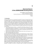
problem is to divide the engine into two parts, into a V-type engine as depicted in Figure
15.10.1. The two sides of the engine are called banks, each containing four cylinders.
Because the total number of cylinders is eight, the engine configuration is commonly
referred to as a V-8.
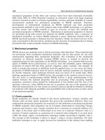
A disadvantage of this engine configuration, however, is that the engine is no longer in
balance, as compared to the straight-eight engine: To see this, consider again the crank
configuration of the straight-eight as listed in Table 15.10.2. Taken by themselves, the first
four cylinders are unbalanced with an unbalanced primary moment perpendicular to the
plane of the cylinders as seen in Table 15.9.6; hence, the second set of four cylinders has
an unbalanced primary moment perpendicular to its plane. With the cylinder planes
themselves being perpendicular, these unbalanced moments no longer cancel but instead
have a vertical resultant as represented in Figure 15.10.2. This unbalance will have a
tendency to cause the engine to oscillate in a yaw mode relative to the engine compartment.
This yawing, however, can often be kept small by the use of motor mounts having high

damping characteristics. Thus, the moment unbalance is usually an acceptable tradeoff in
exchange for obtaining a more compact engine.
TABLE 15.10.2
Engine Balance: Listing of Terms of Eqs. (15.7.8) to (15.7.11) for the Eight-Cylinder Crank Angle
Configuration from Table 15.9.6.
i φφ
φφ
i
(°) cosφφ
φφ
i
sinφφ
φφ
i
cos2φφ
φφ
i
sin2φφ
φφ
i
(i – 1)cosφφ
φφ
i
(i – 1)sinφφ
φφ
i
(i – 1)cos2φφ
φφ
i
(i – 1)sin2φφ

φφ
i
101010 0 0 0 0
2900 1 –10 0 1 –10
3 270 0 –1 –10 0 –2 –20
4 180 –10 10 –30 30
5 180 –10 10 –40 40
6 270 0 –1 –10 0 –5 –50
7900 1 –10 0 6 –60
801010 7 0 7 0
Totals 0 0 0 0 0 0 0 0
FIGURE 15.10.1
A V-type engine.
FIGURE 15.10.2
Unbalance primary moments and
their resultants.
(Resultant)
0593_C15_fm Page 533 Tuesday, May 7, 2002 7:05 AM
534 Dynamics of Mechanical Systems
15.11 Closure
Our analysis shows that if a system is out of balance it can create undesirable forces at
the bearings and supports. If the balance is relatively small, it can often be significantly
reduced or even eliminated by judicious placing of balancing weights.
Perhaps the most widespread application of balancing principles is with the balancing
of internal-combustion engines and with similar large systems. Because such systems have
a number of moving parts, complete balance is generally not possible. Designers of such
systems usually attempt to minimize the unbalance while at the same time making com-
promises or tradeoffs with other design objectives.
We saw an example of such a tradeoff in the balancing of an eight-cylinder engine: the
engine could be approximately balanced if the cylinders were all in a line. This arrange-

ment, however, creates a relatively long engine, not practical for many engine compart-
ments. An alternative is to divide the engine into two banks of four cylinders, inclined
relative to each other (the V-8 engine); however, the engine is then out of balance in yaw
moments, requiring damping at the engine mounts to reduce harmful vibration.
Optimal design of large engines thus generally involves a number of issues that must be
resolved for each individual machine. While there are no specific procedures for such
optimal design, the procedures outlined herein, together with information available in the
references, should enable designers and analysts to reach toward optimal design objectives.
References
15.1. Wilson, C. E., Sadler, J. P., and Michaels, W. J., Kinematics and Dynamics of Machinery, Harper
& Row, New York, 1983, pp. 609–632.
15.2. Wowk, V., Machine Vibrations, McGraw-Hill, New York, 1991, pp. 128–134.
15.3. Paul, B., Kinematics and Dynamics of Planar Machinery, Prentice Hall, Englewood Cliffs, NJ,
1979, chap. 13.
15.4. Mabie, H. H., and Reinholtz, C. F., Mechanisms and Dynamics of Machinery, Wiley, New York,
1987, chap. 10.
15.5. Sneck, H. J., Machine Dynamics, Prentice Hall, Englewood Cliffs, NJ, 1991, pp. 211–227.
15.6. Swight, H. B., Tables of Integrals and Other Mathematical Data, Macmillan, New York, 1057, p. 1.
15.7. Shigley, J. E., and Uicker, J. J., Jr., Theory of Machines and Mechanisms, McGraw-Hill, New York,
1980, p. 499.
15.8. Martin, G. H., Kinematics and Dynamics of Machines, McGraw-Hill, New York, 1982, p. 419.
15.9. Taylor, C. F., The Internal-Combustion Engine in Theory and Practice, Vol. II: Combustion, Fuels,
Materials, Design, MIT Press, Cambridge, MA, 1985, pp. 240–305.
Problems
Section 15.2 Static Balancing
P15.2.1: A 125-lb flywheel in the form of a thin circular disk with radius 1.0 ft and thickness
1.0 in. is mounted on a light (low-weight) shaft which in turn is supported by nearly
0593_C15_fm Page 534 Tuesday, May 7, 2002 7:05 AM
Balancing 535
frictionless bearings as represented in Figure P15.2.1. If the flywheel is mounted off-center

by 0.25 in., what weight should be placed on the flywheel rim, opposite to the off-center
offset, so that the flywheel is statically balanced?
P15.2.2: Repeat Problem P15.2.1 if the flywheel mass is 50 kg, with a radius of 30 cm, a
thickness of 2.5 cm, and an off-center mounting of 7 mm.
P15.2.3: See Problem P15.2.1. Suppose the flywheel shaft has frictionless bearings. What
would be the period of small oscillations?
P15.2.4: Repeat Problem P15.2.3 for the data of Problem P15.2.2.
P15.2.5: See Problem P15.2.3. Suppose a slightly unbalanced disk flywheel, supported in
a light shaft with frictionless bearings, is found to oscillate about a static equilibrium
position with a period of 7 sec. How far is the flywheel mass center displaced from the
shaft axis?
Section 15.3 Dynamic Balancing
P15.3.1: A shaft with radius r of 3 in. is rotating with angular speed Ω of 1300 rpm. Particles
P
1
and P
2
, each with weight w of 2 oz. each, are placed on the surface of the shaft as shown
in Figure P15.3.1. If P
1
and P
2
are separated axially by a distance ᐉ of 12 in., determine
the magnitude of the dynamic unbalance.
P15.3.2: Repeat Problem P15.3.1 if r, w, and ᐉ have the values r = 7 cm, w = 50 g, and
ᐉ = 0.333 m.
P15.3.3: See Problem P15.3.1. Suppose the dynamically unbalanced shaft is made of steel
with a density of 489 lb/ft
3
. Suppose further that it is proposed that the shaft be balanced

by removing material by drilling short holes on opposite sides of the shaft. Discuss the
feasibility of this suggestion. Specifically, if the holes are to be no more than 0.5 in. in
diameter, no more than 0.5 in. deep, and separated axially by no more than 18 in., suggest
a drilling procedure to balance the shaft. That is, suggest the number, size, and positioning
of the holes.
P15.3.4: Repeat Problem P15.3.3 for the shaft unbalance of Problem P15.3.2 if the mass
density of the shaft is 7800 kg/m
3
.
FIGURE P15.2.1
A flywheel on a light shaft in nearly
frictionless bearings.
FIGURE P15.3.1
A rotating shaft with unbalance particles.
1 in.
Flywheel (125 lb)
12 in.
P
P
Ω
ᐉ
1
2
0593_C15_fm Page 535 Tuesday, May 7, 2002 7:05 AM
536 Dynamics of Mechanical Systems
Section 15.4 Dynamic Balancing: Arbitrarily Shaped Rotating Bodies
P15.4.1: Suppose n
1
, n
2

, and n
3
are mutually perpendicular unit vectors fixed in a body B,
and suppose that B is intended to be rotated with a constant speed Ω about an axis X
which passes through the mass center G of B and which is parallel to n
1
. Let n
1
, n
2
, and
n
3
be nearly parallel to principal inertia directions of B for G so that the components I
ij
of
the inertia dyadic of B for G relative to n
1
, n
2
, and n
3
are:
Show that with this configuration and inertia dyadic that B is dynamically out of balance.
Next, suppose we intend to balance B by the addition of two 12-oz. weights P and
placed opposite one another about the mass center G. Determine the coordinates of P
and relative to the X-, Y-, and Z-axes with origin at G and parallel to n
1
, n
2

, and n
3
.
P15.4.2: Repeat Problem P15.4.1 if the inertia dyadic components are:
and if the masses of P and are each 0.5 kg.
P15.4.3: Repeat Problems P15.4.1 and P15.4.2 if B is rotating about the Z-axis instead of
the X-axis.
Section 15.5 Balancing Reciprocating Machines
P15.5.1: Suppose the crank AB of a simple slider/crank mechanism (see Figures 15.5.1 and
P15.5.1, below) is modeled as a rod with length of 4 in. and weight of 2 lb. At what distance
away from A should a weight of 4 lb be placed to balance AB?
P15.5.2: See Problem P15.5.1. Suppose is to be 1.5 in. What should be the weight of the
balancing mass ?
P15.5.3: Repeat Problem P15.5.1 if rod AB has length 10 cm and mass 1 kg.
P15.5.4: Consider again the simple slider/crank mechanism as in Figure P15.5.4, this time
with an objective of eliminating or reducing the primary unbalancing force as developed
in Eq. (15.5.23). Specifically, let the length r of the crank arm be 4 in., the length ᐉ of the
connecting rod be 9 in., the weight of the piston C be 3.5 lb, and the angular speed w of
FIGURE P15.5.1
A simple slider crank mechanism.
I
ij
=
−
−−
−











18 01 025
01 12 015
0 25 0 15 6



slug ft
2
ˆ
P
ˆ
P
I
ij
=
−−
−
−











30 02 03
02 20 025
03 025 10



kg m
2
ˆ
P
ˆ
r
C
r
m
A
B
ˆ
ˆ
B
ˆ
r
ˆ
m
B
0593_C15_fm Page 536 Tuesday, May 7, 2002 7:05 AM

Balancing 537
the crank be 1000 rpm. Determine the weight (or mass ) of the balancing weight to
eliminate the primary unbalance if the distance h of the weight from the crank axis is 3
in. Also, determine the maximum secondary unbalance that remains and the maximum
unbalance in the Y-direction created by the balancing weight.
P15.5.5: Repeat Problem P15.5.4 if the balancing weight compensates for only (a) 1/2 and
(b) 2/3 of the primary unbalance.
P15.5.6: Repeat Problems P15.5.4 and P15.5.5 if r is 10 cm,
ᐉ is 25 cm, h is 5 cm, and the
mass of C is 2 kg.
Section 15.6 Lanchester Balancing
P15.6.1: Verify Eqs. (15.6.1), (15.6.2), and (15.6.3).
P15.6.2: Observe that the geometric parameters of Eq. (15.6.5) are such that the Lanchester
balancing mass m
ᐉ
need only be a fraction of the piston mass m
C
. Specifically, suppose
that (r/ᐉ) is 0.5 and (ξ/r) is also 0.5. What, then, is the mass ratio m
ᐉ
/m
C
?
Sections 15.7, 15.8, 15.9 Balancing Multicylinder Engines
P15.7.1: Consider a three-cylinder, four-stroke engine. Following the procedures outlined
in Sections 15.7, 15.8, and 15.9, develop a firing order and angular positioning to optimize
the balancing of the engine.
FIGURE P15.5.4
A slider crank mechanism.
A

B
θ
Y
r
ᐉ
C(m )
C
X
w
ˆ
m
0593_C15_fm Page 537 Tuesday, May 7, 2002 7:05 AM
0593_C15_fm Page 538 Tuesday, May 7, 2002 7:05 AM

539

16

Mechanical Components: Cams

16.1 Introduction

In this chapter, we consider the design and analysis of cams and cam–follower systems.
As before, we will focus upon basic and fundamental concepts. Readers interested in
more details than those presented here may want to consult the references at the end
of the chapter.
A cam (or

cam-pair

) is a mechanical device intended to transform one kind of motion
into another kind of motion (for example, rotation into translation). In this sense, a cam
is primarily a kinematic device or mechanism. The most common cam-pairs transform
simple uniform (constant speed) rotation into translation (or rectilinear motion).
Figure 16.1.1 shows a sketch of such a device. In such mechanisms, the actuator (or active)
component (in this case, the rotating disk) is called the

cam

. The responding (or passive)
component is called the

follower

.
Some cam-pairs simply convert one kind of translation into another kind of translation,
as in Figure 16.1.2. Here, again, the actuator or driving component is the cam and the
responding component is the follower. An analogous cam-pair that transforms simple
rotation into simple rotation is a pair of meshing gears depicted schematically in
Figure 16.1.3. Because gears are used so extensively, they are usually studied separately,
which we will do in the next chapter. Here, again, however, the actuator gear is called the

driver

and the responding gear is called the

follower

. Also, the smaller of the gears is called
the

pinion

and the larger is called the

gear

.
To some extent, the study of cams employs different procedures than those used in our
earlier chapters; the analysis of cams is primarily a kinematic analysis. Although the study
of forces is important in mechanism analyses, the forces generated between cam–follower
pairs are generally easy to determine once the kinematics is known. The major focus of
cam analysis is that of cam design. Whereas in previous chapters we were generally given
a mechanical system to analyze, with cams we are generally given a desired motion and
asked to determine or design a cam–follower pair to produce that motion.
In the following sections, we will consider the essential features of cam and follower
design. We will focus our attention upon simple cam pairs as in Figure 16.1.1. Similar
analyses of more complex cam mechanisms can be found in the various references. Before
directing our attention to simple cam pairs, it may be helpful to briefly review configu-
rations of more complex cam mechanisms. We do this in the following section and then
consider simple cam–follower design in the subsequent sections.

0593_C16_fm Page 539 Tuesday, May 7, 2002 7:06 AM

540

Dynamics of Mechanical Systems

16.2 A Survey of Cam Pair Types

As noted earlier, the objective of a cam–follower pair is to transform one kind of motion
into another kind of motion. As such, cam-pairs are kinematic devices. When, in addition
to transforming and transmitting motion, cam-pairs are used to transmit forces, they are
called

transmission

devices.
There are many ways to transform one kind of motion into another kind of motion.
Indeed, the variety of cam–follower pair designs is limited only by one’s imagination. In
addition to those depicted in Figures 16.1.1, 16.1.2, and 16.1.3, Figures 16.2.1, 16.2.2, and
16.2.3 depict other common types of cams. Figures 16.2.4 and 16.2.5 depict various common

FIGURE 16.1.1

A simple cam–follower pair.

FIGURE 16.1.2

A translation to translation cam–follower pair.

FIGURE 16.1.3

A gear pair.

FIGURE 16.2.1

Cam–follower with cam–follower track.

FIGURE 16.2.2

Cylindrical cam with cam–follower track.
Follower
Cam
Follower
Cam
Driver
Follower
Cam Follower
Cam Follower Track
Cam
Rotation
Rotation
Cam Follower Track
Cam Follower

0593_C16_fm Page 540 Tuesday, May 7, 2002 7:06 AM

Mechanical Components: Cams

541
follower types. Figures 16.2.2 and 16.2.3 show that cam–follower pairs may be used not
only for exchanging types of planar motion but also for converting planar motion into
three-dimensional motion.
In the following sections, we will direct our attention to planar rotating cams (or

radial
cams

) with translating followers as in Figure 16.2.4. Initially, we will consider common

nomenclature and terminology for such cams.

16.3 Nomenclature and Terminology for Typical Rotating Radial Cams
with Translating Followers

Consider a radial cam–follower pair as in Figure 16.3.1 where the axis of the follower shaft
intersects the axis of rotation of the cam. Let the follower shaft be driven by the cam

FIGURE 16.2.3

Conical cam with cam–follower.

FIGURE 16.2.4

Types of translation followers.

FIGURE 16.2.5

Types of rotation followers.
Cam Follower Track
Cam Follower
Point Follower Plane Follower Roller Follower
Slider Follower
Roller Follower

0593_C16_fm Page 541 Tuesday, May 7, 2002 7:06 AM

542

Dynamics of Mechanical Systems

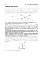
through a follower wheel as shown. Figure 16.3.2 shows the commonly employed termi-
nology and nomenclature of the radial cam–follower pair [16.1]. Brief descriptions of these
items follow:
• Cam profile — contact boundary of the rotating cam
• Follower wheel — rolling wheel of the follower contacting the cam profile to
reduce wear and to provide smooth operation
• Trace point — center of rolling follower wheel; also, point of

knife-edge

follower
• Pitch curve — path of the trace point
• C — typical location of the trace point on the pitch curve
•

θ

— pressure angle
Observe the pressure angle in Figure 16.3.2. It is readily seen that the pressure angle is
a measure of the lateral force exerted by the cam on the follower. Large lateral forces (as
opposed to longitudinal or axial forces) can lead to high system stress and eventually
deleterious wear. A large pressure angle

θ

can create large lateral forces. Specifically, the
lateral force is proportional to sin

θ

.
Observe further in Figure 16.3.2 that if the cam profile is circular the pressure angle is
zero. In this case, no lateral forces are exerted on the follower by the cam. However, with
the circular profile, no longitudinal force will be exerted on the follower, so the follower
will remain stationary. A stationary follower corresponds to a

dwell

region for the cam.

FIGURE 16.3.1

A radial cam–follower pair.

FIGURE 16.3.2

Radial cam–follower pair terminology and nomenclature.

Direction of
Follower Motion
Cam Normal
Follower
Trace Point
Follower Wheel
Cam Profile
Pitch Curve

0593_C16_fm Page 542 Tuesday, May 7, 2002 7:06 AM

Mechanical Components: Cams

543
These observations show that there is no follower movement without a nonzero pressure
angle; hence, a cost of follower movement is the lateral force generated by the pressure angle.
Thus, cam designers generally attempt to obtain the desired follower motion with the smallest
possible pressure angle. This is usually accomplished by a large cam, as space permits.
Finally, observe that the follower wheel simply has the effect of enlarging the cam profile
creating the

pitch curve

, with the follower motion then defined by the movement of the
trace point.

16.4 Graphical Constructions: The Follower Rise Function

The central problem confronting the cam designer is to determine the cam profile that
will produce a desired follower movement. To illustrate these concepts and some graphical
design procedures, consider again the simple knife-edge radial follower pair of
Figure 16.4.1. Let the cam profile be represented analytically as (see Figure 16.4.2):
(16.4.1)
where

r

and

θ

are polar coordinates of a typical point

P

on the cam profile. The angle

θ

may also be identified with the rotation angle of the cam. Thus, given

f

(

θ

), we know

r

as
a function of the rotation angle. Then with the knife-edge follower, we can identify

r

with
the movement of the follower.
If the angular speed

ω

of the cam (

ω

= ) is constant, the speed

v

of the follower is:
(16.4.2)
and the acceleration

a

of the follower is:
(16.4.3)

FIGURE 16.4.1

Knife-edge radial cam–follower pair.

FIGURE 16.4.2

Polar coordinates of a cam profile.
rf=
()
θ
˙
θ

v r dr dt df dt
df
d
d
dt
df
d
== = = =
˙
θ
θ
ω
θ
ar
d
dt
df
d
d
dt
df
d
d
d
df
d
d
dt
df
d

==




=




=










=
˙˙
ω
θ
ω
θ
ω
θθ
θ

ω
θ
2
2
2
Y
X
P
O
r
θ

0593_C16_fm Page 543 Tuesday, May 7, 2002 7:06 AM

544

Dynamics of Mechanical Systems

Let

r

min

be the minimum value of

r

in Eq. (16.4.1). Let

h

be the difference between

r

and

r

min

at any cam position: That is, let
(16.4.4)
Then,

h

(

θ

) represents the rise (height) of the follower above its lowest position.
We can obtain a graphical representation of

h

(

θ

) by dividing the cam into equiangular
segments and then by constructing circular arcs from the segment line/cam profile inter-
section to the vertical radial line. Then, horizontal lines from these intersections determine
the

h

(

θ

) profile, as illustrated in Figure 16.4.3.
By inspecting the construction of Figure 16.4.3, we see that given the cam profile it is
relatively easy — at least, in principle — to obtain the follower rise function

h

(

θ

). The
inverse problem, however, is not as simple; that is, given the follower rise function

h

(

θ

),
determine the driving cam profile. This is a problem commonly facing cam designers
which we discuss in the following section.

16.5 Graphical Constructions: Cam Profiles

If we are given the follower rise function

f

(

θ

), we can develop the cam profile by reversing
the graphical construction of the foregoing section. To illustrate this, consider a general
follower rise function as in Figure 16.5.1.
Next, we can construct the cam profile by first selecting a minimum cam radius

r

min

.
Then, the cam radius at any angular position is defined by Figure 16.5.1. Graphically, this
may be developed by constructing a circle with radius

r

min

and then by scaling points on
radial lines according to the follower rise function. To illustrate this, let this minimum
radius circle (called the

base circle

) and the radial lines be constructed as in Figure 16.5.2.
Next, let the follower rise be plotted on radial lines according to the angular position as

FIGURE 16.4.3

Graphical construction of follower rise profile.
hrr f r h=− =
()
−=
()
min min
θθ

0593_C16_fm Page 544 Tuesday, May 7, 2002 7:06 AM

Mechanical Components: Cams

545
in Figure 16.5.3 where, for illustrative purposes, we have used the data of Figure 16.5.1.
Then, by fitting a curve through the plotted points on the radial line we obtain the cam
profile as in Figure 16.5.3. The precision of this process can be improved by increasing the
number of radial lines.

Although this procedure seems to be simple enough, hidden difficulties may emerge in
actual construction, including the effects of differing cam–follower geometries and the
more serious problem of obtaining a cam profile that may produce undesirable accelera-
tions of the follower. We discuss these problems and their solutions in the following
sections.

16.6 Graphical Construction: Effects of Cam–Follower Design

In reviewing the procedures of the two foregoing sections, we see and recall from Figure
16.4.1 that our discussions assumed a simple knife-edge radial follower. If the follower
design is modified, however, the graphical procedures will generally need to be modified
as well.
To illustrate these changes, consider again an elliptical cam profile for which the follower
is no longer radial but instead is offset from the cam rotation axis. Also, let the contact
surface between the follower and cam be an extended flat surface as in Figure 16.6.1.

FIGURE 16.5.1

A typical follower rise function.

FIGURE 16.5.2

Base circle and radial lines.

FIGURE 16.5.3

Cam profile for follower rise function of
Figure 16.5.1.
Base
Circle

Cam Profile

0593_C16_fm Page 545 Tuesday, May 7, 2002 7:06 AM

546

Dynamics of Mechanical Systems

If, as before, we attempt to determine the follower rise function (assuming constant cam
angular speed) by considering equiangular radial lines, we see that, due to the offset, the
follower axis will not coincide with the radial lines. Also, due to the flat follower surface,
we see that the base of the follower at the axis of the follower will not, in general, be in
contact with the cam profile (see Figure 16.6.2).
A question that arises then is how do these geometrical changes affect the graphical
construction of the follower rise profile as in Figure 16.4.3? To answer this question,
consider again constructing radial lines on the cams as in Figure 16.4.3 and as shown
again here in Figure 16.6.3.
Next, for each radial line let a profile of the follower be superposed on the figure such
that the axis of the follower is parallel to the radial line but offset from it by the offset of
the follower axis and the cam axis. Let the follower profile be placed so that the flat edge

FIGURE 16.6.1

An offset flat-surface follower.

FIGURE 16.6.2

Contact between cam and follower at a typical cam
orientation.

FIGURE 16.6.3

Cam profile with superposed radial lines.

FIGURE 16.6.4

Representation of the follower at various positions
about the cam profile.

0593_C16_fm Page 546 Tuesday, May 7, 2002 7:06 AM

Mechanical Components: Cams

547
is tangent to the cam profile. A representation of this procedure at 45°-angle increments
is shown in Figure 16.6.4.
Finally, let the points of tangency between the flat edge of the follower and the cam
profile be used to develop the follower rise function using the procedure of Figure 16.4.3
and as demonstrated in Figure 16.6.5.
The inverse problem of determining the cam profile when given the follower rise
function is a bit more difficult, but it may be solved by following similar procedures to
those of Figures 16.6.3, 16.6.4, and 16.6.5. (As noted earlier, this problem is of greater
interest to designers, whereas the problem of determining the follower rise function is of
greater interest to analysts.)
To illustrate the procedure, suppose we are given a follower rise function as in Figure
16.5.1 and as shown again in Figure 16.6.6. To accommodate such a function with an offset
flat surface follower as in Figure 16.6.1, we need to slightly modify the procedure of
Section 16.5 in Figures 16.5.2 and 16.5.3. Specifically, instead of constructing radial lines
through the cam axis as in Figure 16.5.2, we need to account for the offset of the follower
axis. This means that, instead of radial lines through the cam axis, we need to construct

tangential lines to a circle centered on the cam axis with radius equal to the offset and
thus tangent to the follower axis.
To see this consider again the representation of the offset flat surface follower of
Figure 16.6.1 and as shown in Figure 16.6.7. Let the offset between the follower and cam

FIGURE 16.6.5

Graphical construction of follower rise profile.

FIGURE 16.6.6

A typical follower rise function.

0593_C16_fm Page 547 Tuesday, May 7, 2002 7:06 AM

548

Dynamics of Mechanical Systems

rotation axis be

ρ

as shown. Next, construct a circle with radius

ρ

and with tangent lines
representing the follower axis and placed at equal interval angles around the circle as
shown in Figure 16.6.8.

The third step is to select a base circle radius, as before, and to superimpose it over the
offset axes circle (coincident centers) as in Figure 16.6.9. Fourth, using the follower rise
function of Figure 16.6.6, we can use the curve ordinates of the various cam rotation angles
as the measure of the follower displacement above the base circle, along the corresponding
radial lines of Figure 16.6.9. Figure 16.6.10 shows the location of these displacement points.
Finally, by sketching the flat surface of the follower placed at these displacement points
we form an

envelope

[16.2] of the cam profile. That is, the flat follower surfaces are tangent
to the cam profile. Then, by sketching the curve tangent to these surfaces, we have the
cam profile as shown in Figure 16.6.11.
Observe in this process that accuracy is greatly improved by increasing the number of
angle intervals. Observe further that, while this process is, at least in principle, the same
as that of the foregoing section (see Figure 16.5.3), the offset of the follower axis and the
flat surface of the follower require additional graphical construction details. (One effect

FIGURE 16.6.7

Offset flat surface follower of Figure 16.6.1.

FIGURE 16.6.8

Offset axes circle and tangent line.

FIGURE 16.6.9

Base circle superposed over offset axis circle.
ρ

0593_C16_fm Page 548 Tuesday, May 7, 2002 7:06 AM

Mechanical Components: Cams

549
of this is that the cam profile can fall inside the base circle as seen in Figure 16.6.11.) Finally,
observe that, although the cam profiles of Figures 16.5.3 and 16.6.11 are not identical, they
are similar.

16.7 Comments on Graphical Construction of Cam Profiles

Although the foregoing constructions are conceptually relatively simple, difficulties are
encountered in implementing them. First, because they are graphical constructions, their
accuracy is somewhat limited — although emerging computer graphics techniques will
undoubtedly provide a means for improving the accuracy. Next, analyses assuming point
contact between the cam and follower (as in Sections 16.4 and 16.5) may produce cam
profiles that are either impractical or incompatible with roller-tipped followers. For exam-
ple, for an arbitrary follower rise function, it is possible to obtain cam profiles with cusps
or concavities as in Figure 16.7.1. Finally, if the cam is rotating rapidly (as is often the

FIGURE 16.6.10

Follower displacement points relative to the base circle.

FIGURE 16.6.11

Envelope of follower flat defining the cam profile.

0593_C16_fm Page 549 Tuesday, May 7, 2002 7:06 AM

550

Dynamics of Mechanical Systems

case with modern mechanical systems), the cam profile may create very large follower
accelerations. These accelerations in turn may lead to large and potentially destructive
inertia forces. In the next section, we consider analytical constructions intended to over-
come these difficulties.

16.8 Analytical Construction of Cam Profiles

As with graphical cam profile construction, analytical profile construction has the same
objective; that is, given the follower motion, determine the cam profile that will produce
that motion. Because the follower motion may often be represented in terms of elementary
functions, it follows that the cam profile may also often be represented in terms of ele-
mentary functions. When this occurs, the analytical method has distinct advantages over
the graphical method. Conversely, if the follower motion cannot be represented in terms
of elementary functions, the analytical approach can become unwieldy and impractical,
necessitating the use of numerical procedures and approximations. Also, as we will see,
the design of cam profiles with elementary functions may create undesirable inertia forces
with high-speed systems.
With these possible deficiencies in mind, we outline the analytical construction in the
following text. As with the graphical construction, we develop the fundamentals using
the simple planar cam–follower pair, with the follower axis intersecting the rotation axis
of the cam as in Figure 16.8.1. Also, we will assume the cam rotates with a constant angular
speed

ω

0

.
In many applications, the follower is to remain stationary for a fraction of the cam
rotation period. After passing through this stationary period, the follower is then generally
required to rise away from this stationary position and then ultimately return back to the
stationary position. Figure 16.8.2 shows such a typical follower motion profile. The sta-
tionary positions are called

periods of dwell

for the follower and, hence, also for the cam.
The principle of analytical cam profile construction is remarkably simple. The follower
rise function

h

(

θ

) (as shown in Figure 16.8.2) is directly related to the cam profile function.
To see this, note that, because the cam is rotating at a constant angular speed

ω

0
, the
angular displacement θ of the cam is a linear function of time t. That is,
(16.8.1)

where the initial angle θ
0
may conveniently be taken as zero without loss of generality.
FIGURE 16.7.1
Incompatible and impractical cam profiles for a roller follower.
(a) (b)
If thenωθ θωθ
000
==+ddt t,
0593_C16_fm Page 550 Tuesday, May 7, 2002 7:06 AM
Mechanical Components: Cams 551
Next, because the follower rise h is often expressed as a function of time t, say h(t), we
can solve Eq. (16.8.1) for t (t = θ/ω
0
) and then express the follower displacement as a
function of the rotation angle θ as in Figure 16.8.3. Then, in view of the graphical con-
structions of the foregoing sections and in view of Figure 16.8.1, we see that the follower
rise function is simply the deviation of the cam profile from its base circle. That is, if the
cam profile is expressed in polar coordinates as r(θ), then r(θ) and h(θ) are related as:
(16.8.2)
where r
0
is the base circle radius.
16.9 Dwell and Linear Rise of the Follower
To illustrate the application of Eq. (16.8.2), suppose the follower displacement is in dwell.
That is, let the rise function hθ be zero as in Figure 16.9.1. Then, the cam profile r(θ) has
the simple form:
(16.9.1)
That is, the cam profile is circular, with radius equal to the base circle, and no follower
motion is generated.

FIGURE 16.8.1
Knife-edge radial cam–follower
pair.
FIGURE 16.8.2
Typical follower rise function.
FIGURE 16.8.3
Follower displacement as a function
of the cam rotation angle θ.
Dwell
Dwell
Dwell
Cam Rotation (Period T)
Follower
Rise
h(t)
0
T
t
rrhθθ
()
=+
()
0
rrθ
()
=
()
0
a constant
0593_C16_fm Page 551 Tuesday, May 7, 2002 7:06 AM

552 Dynamics of Mechanical Systems
Next, suppose the follower rise function is not zero but instead is still a constant (say,
h
0
) as in Figure 16.9.2. In this case, the follower is still in dwell, but after a displacement
(or rise) of h
0
. From Eq. (16.8.2) the cam profile is then:
(16.9.2)
Here, again, the cam profile is circular with a radius h
0
greater than the base circle radius.
Next, suppose the rise of the follower increases linearly with time (or cam rotation) as
in Figure 16.9.3. If the follower rise is to begin at θ = θ
1
, then the slope of the rise is:
(16.9.3)
The follower displacement may then be expressed in the form:
(16.9.4)
FIGURE 16.9.1
A zero or dwell follower rise function.
FIGURE 16.9.2
A nonzero dwell follower rise function.
FIGURE 16.9.3
A linear rise in the follower displacement.
FIGURE 16.9.4
Linear rise over quarter cam angle.
Dwell
Follower
Rise

h(θ)

Cam Rotation θ
Dwell
Follower
Rise
h(θ)

Cam Rotation θ
h
O
Dwell
Follower
Rise

h
h
Dwell
Linear
Rise
θ θ
θ
2
1
2
1
rrhθ
()
=+
()

00
a constant
slope =
D
hh
m
21
21
−
−
=
θθ
h
h
m
h
θ
θθ
θθ θ θθ
θθ
()
=
≤
−
()
≤≤
≥






11
11 2
22
0593_C16_fm Page 552 Tuesday, May 7, 2002 7:06 AM
Mechanical Components: Cams 553
Hence, from Eq. (16.8.2) the cam profile radius r(θ) is:
(16.9.5)
Using Eq. (16.9.4) produces a profile as in Figure 16.9.4, where a linearly increasing radius
is shown for 90° of the cam angle.
16.10 Use of Singularity Functions
The foregoing analysis may be facilitated by the use of singularity or delta functions. To
develop this idea, let us first introduce the step function δ
1
(x) defined as (see References
16.3 to 16.6):
(16.10.1)
where δ
1
(0) is left undefined (or, on occasion, defined as 1/2). Then, by shifting the
independent variable, we have:
(16.10.2)
We can immediately apply Eq. (16.10.2) with the follower rise function h(θ). For example,
consider the linear rise function of Eq. (16.9.4):
(16.10.3)
Then, by using Eq. (16.10.2), the follower rise function may be written as:
(16.10.4)
By integrating, we may generalize the definition of Eq. (16.10.1) and thus introduce
higher order step-type functions (or singularity [16.6] functions) as:

(16.10.5)
where δ
2
(0) is defined as 0. Similarly, we have:
rrhθθ
()
=+
()
0
δ
1
00
10
x
x
x
()
=
<
>



D
δ
1
0
1
xa
xa

xa
−
()
=
<
>



h
h
m
h
θ
θθ
θθ θ θθ
θθ
()
=
≤
−
()
≤≤
≥





11

11 2
22
hhm
hhh
θθθδθθδθθ
θθ
θθ
δθ θ δθ θ
()
=+ −
()
−
()
−−
()
[]
=+ −
()
−
−






−
()
−−
()

[]
111112
121
1
21
1112
δδ
21
0
00
xxx
xx
x
()
=
()
=
>
<



D
0593_C16_fm Page 553 Tuesday, May 7, 2002 7:06 AM
554 Dynamics of Mechanical Systems
(16.10.6)
(16.10.7)
(16.10.8)
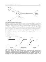
Observe that the definitions:
(16.10.9)

allow the functions to be continuous at x = 0.
Graphically, these functions may be represented as in Figure 16.10.1. Observe that except
for δ
1
(x) all the functions are continuous at x = 0.
Observe further that just as δ
n+1
(x) represents the integration (or antiderivative) of δ
n
(x),
it follows that δ
n
(x) is the derivative of δ
n+1
(x). This raises the question, however, as to the
derivative of δ
1
(x). From the definition of Eq. (16.10.1), we see that, if x ≠ 0, then dδ
1
(x)/dx
is zero. At x = 0, however, the derivative is undefined, representing an infinite change in
the function. Thus, we have:
(16.10.10)
δ
0
(x) is often referred to as Dirac’s delta function — analogous to Kronecker’s delta
function of Section 2.6. The analogy is seen through the “sifting” or “substitution” property
of the functions. Recall from Eq. (2.6.7) that we have:
(16.10.11)
Similarly, it is seen (see References 16.1 to 16.5) that:

(16.10.12)
or
(16.10.13)
Interpreting an integral as a sum, we see that Eqs. (16.10.11) and (16.10.11) are simply
discrete and continuous forms of the same procedure with analogous results.
δδ δ
3
2
1
2
3
2
20
00
00xx x
xx
x
()
=
()
()
=
>
<
()
=



DD

,
δδ δ
4
3
1
3
4
6
60
00
00xx x
xx
x
()
=
()
()
=
>
<
()
=



DD
,
δδ δ
n
n

n
n
xxnx
xn x
x
++
()
=
()
()
=
>
<
()
=



11 1
0
00
00
DD
!
!
,
δδ δδ
23 1
00 0 00
()

=
()
=…=
()
=
()
=
+nn
d x dx x
x
x
δδ
10
00
0
()
=
()
=
≠
∞=



D

δ
ij j i
vv=
fx xdx f b

b
b
() ()
=
()
>
()
−
∫
δ
0
00
fx x adx fa b a
b
b
()
−
()
=
()
>
()
−
∫
δ
0
0593_C16_fm Page 554 Tuesday, May 7, 2002 7:06 AM
Mechanical Components: Cams 555
The functions δ
2

(x), δ
3
(x), δ
4
(x),…, δ
n+1
(x) of Eqs. (16.10.5) through (16.10.8), as well as
δ
0
(x) of Eq. (16.10.10), may also be represented with the independent variable shifted as
in Eq. (16.10.2). That is,
(16.10.14)
and
(16.10.15)
From Eq. (16.10.15), we see that δ
0
(x – a) may be represented graphically as in
Figure 16.10.2.
Symbolically, or by appealing to generalized function theory [16.5], we may develop
derivatives of Dirac’s delta function as:
(16.10.16)
where δ
–1
(x) has the form of an impulsive doublet function as in Figure 16.10.3. (Graphical
representations of the higher order derivatives are not as readily obtained, thus the graph-
ical representations of the higher order derivatives are not as helpful.)
There has been extensive application of these influence or interval functions in structural
mechanics — particularly in beam theory (see, for example, Reference 16.6). For cam profile
analysis, they may be used to conveniently define the profile, as in Eq. (16.10.4). The
principal application of the functions in cam analysis, however, is in the differentiation of

FIGURE 16.10.1
Graphical form of the singularity function.
1
0
x
δ (x)
1
0
x
δ (x)
2
0
x
δ (x)
3
0
x
δ (x)
n
. . .
δδ
δδ
23
2
4
3
1
0
2
0

6
00
xa
xa xa
xa
xa
xa xa
xa
xa
xa xa
xa
xa
xa n xa
xa
n
n
−
()
=
−≥
≤



−
()
=
−
()
≥

≤





−
()
=
−
()
≥
≥





…−
()
=
−
()
≥
≤






+
, ,
,,
!
δ
0
0
xa
xa
xa
−
()
=
≠
∞=



dxdx x d xdx x
d x dx x
n
n
δδδ δ
δδ
0112
1
()
=
() ()
=

()
…
()
=
()
−− −
−
−+
()
,

0593_C16_fm Page 555 Tuesday, May 7, 2002 7:06 AM
556 Dynamics of Mechanical Systems
the follower rise function, providing information about the follower velocity, acceleration,
and rate of change of acceleration (jerk).
To demonstrate this, consider again the piecewise-linear follower rise function of Figure
16.9.3 and as expressed in Eq. (16.10.4):
(16.10.17)
where as before m is (h
2
– h
1
)/(θ
2
– θ
1
) (see Figure 16.9.3). The velocity v and the acceleration
a of the follower are then:
(16.10.18)
and

(16.10.19)
where, as before, we have assumed the cam rotation dθ/dt (= ω) to be constant. Then, by
substituting from Eq. (16.10.17) into (16.10.18) and (16.10.19), we find v and a to be:
(16.10.20)
and
(16.10.21)
We can readily see that the final terms in both Eqs. (16.10.20) and (16.10.21) are zero. To
see this, consider first the expression xδ
0
(x). If x is not zero, then δ
0
(x) and thus xδ
0
(x) are
FIGURE 16.10.2
Representation of Dirac’s delta function.
FIGURE 16.10.3
Representation of the derivative of Dirac’s delta
function.
0
a
x
δ (x - a)
0
0
a
x
δ (x - a)
-1
hhmθθθδθθδθθ

()
=+ −
()
−
()
−−
()
[]
111112
v
dh
dt
dh
d
d
dt
dh
d
== =
θ
θ
ω
θ
a
dh
dt
d
dt
dh
dt

d
d
dh
dt
d
dt
d
d
dh
d
dh
d
==




=




=











=
2
2
2
2
2
θ
θ
θ
ω
θ
ωω
θ
vm m=−
()
−−
()
[]
+−
()
−
()
−−
()
[]
ωδθθ δθθ ω θθδθθ δθθ
1112 10102

am=−
()
−−
()
[]
+−
()
−
()
−−
()
[]
−−
2
2
0102 11112
ω δθθ δθθ ωθθδ θθ δθθ
0593_C16_fm Page 556 Tuesday, May 7, 2002 7:06 AM