Automation and Robotics Part 4 docx

Vision Guided Robot Gripping Systems


69
obtained with and without the distortion parameters. Although distortions seemed not to
influence the accuracy for the lens focal length of 16 mm, the authors suggest that they
should be included in the camera model when the camera is equipped with lenses of shorter
focal lengths.
The figures show that the measuring accuracy of the system without the corrected hand-eye
parameters is unsatisfactory for Baselines 1 and 3. The desired accuracy was achieved for
Baseline 2, though here the camera-checkerboard transformations computed by MCT had
very small errors as compared to those obtained for the other two baselines. Yet, the system
with Baseline 2 had the best accuracy because the distances from the Camera 1 to the Object
CS were relatively smaller in this configuration. Fig. 12 shows the distances between these
two CSs varying from 250 mm to 600 mm, while we set the focus of the cameras at the
distance of 400 mm. Although images were blurred at minimal and maximal distances, such
deviations proved to be acceptable. Not surprisingly, Baseline 3, the shortest one, produced
the worst accuracy.


Automation and Robotics


70



Fig. 11. Repeatability error of the kx, ky, kz coordinates and the A, B, C angles for Baselines
1, 2, 3 : square – with the distortion coefficients and with hand-eye corrections; circle –
without the distortion coefficients and with the hand-eye corrections; triangle – with the

distortion coefficients and without the hand-eye corrections

The proposed manual calibration of the stereovision system satisfied the criterions of
repeatability of measurements. Although there are some errors shown in Fig. 11 that exceed
the desired accuracy, it has to be noticed that some pictures were taken at very acute angles.
In overall, the camera’s yaw angle varied between -50 and +100 deg and the pitch angle
varied between -60 and +40 deg throughout the whole test, what far exceeds the real
working conditions. Moreover, the image data were collected for GA only at the first OP for
each baseline (marked as blue rectangles in the figures) and they were very noisy in several
cases. We suppose that noise must have decreased the GA’s efficiency in searching for the
best solutions, but the evolutionary approach itself allowed preserving stability and
robustness of the ultimate robotic system.
Vision Guided Robot Gripping Systems


71

Fig. 12. Distance between the origins of the Object CS and the Camera 1 CS for each VP
6. Conclusion and future work
A manipulator equipped with vision sensors can be ‘aware’ of the surrounding scene, what
admits of performing tasks with higher flexibility and efficiency. In this chapter a robotic
system with stereo cameras has been presented the purpose of which was to release humans
from handling (picking, moving, etc.) non-constrained objects in a three-dimensional space.
In order to utilize image data, a pinhole camera model has been introduced together with a
“Plumb Bob” model for lens distortions. A precise description of all parameters has been
given. Two conventions (i.e. the Euler-angle and the unit quaternion notations) have been
presented for describing the orientation matrix of rigid-body transformations that are
utilized by leading robot manufacturers. The problem of 3D object pose estimation has been
explained based on retrieved information from single and stereo images. Epipolar geometry
of stereo camera configurations has been analyzed to explain how it can be used to make

image processing more reliable and faster. We have outlined certain pose estimation
algorithms to provide the reader with a wide integrated spectrum of methods utilized in
robot positioning applications when considering specific constraints (like analytical, or
iterative). Moreover, we have also supplied various references to other algorithms. Two
methods for a three-dimensional robot positioning system have been developed and
bridged with the object pose estimation algorithms. Singularities of the robot positioning
systems have been indicated, as well.
A challenging task has been to find a hand-eye transformation of the system, i.e. the
transformation between a camera and a robot end-effector. We have explained the classic
approach by Tsai and Lenz solving this problem and have used a Matlab Calibration
Toolbox to perform calibration. We have extended this approach by utilizing a genetic
algorithm (GA) in order to improve the system measurement precision in the sense of
satisfactory repeatability of positioning the robotic gripper. We have then outlined other
calibration algorithms and suggested an automated calibration as a step towards making the
entire system autonomous and reliable.
The experimental results obtained have proved that our GA-based calibration method yields
the system precision of ±1 mm and ±1 deg, thus satisfying the industrial demands on the
accuracy of automated part acquisition. A future research effort should be placed on (
•)
optimization of the mathematical principles for positioning the robot through some
orthogonality constraints of rotation to increase the system’s accuracy, (
•) development of a
Automation and Robotics


72
method for computing 3D points using two non-overlapping images (to be utilized for large
objects), (
•) implementation of a hand-eye calibration method based on the structure-from-
motion algorithms, and (

•) implementation of algorithms for tracking objects.
7. References
Andreff, N.; Horaud, R. & Espiau, B. (2001). Robot hand-eye calibration using structure-
from-motion. The International Journal of Robotics Research, vol. 20, no. 3, pp. 228-248
Daniilidis, K. (1998). Hand-Eye Calibration Using Dual Quaternions, GRASP Laboratory,
University of Pennsylvania, PA (USA)
Fischler, M.A. & Bolles, R.C. (1981). Random sample consensus: A paradigm for model
fitting with applications to image analysis and automated cartography. Graphics and
Image Processing, vol. 24, no. 6, pp. 381-395
Gruen, A.W. (1985). Adaptive least squares correlation: A powerful image matching
technique. South African Journal of Photogrammetry, Remote Sensing and Cartography,
vol. 14, no. 3, pp. 175-187
Haralick, R.M.; Joo, H.; Lee, C.; Zhuang, X.; Vaidya, V.G. & Kim, M.B. (1989). Pose
estimation from corresponding point data. IEEE Transactions on Systems, Man and
Cybernetics, vol. 19, no. 6, pp. 1426-1446
Horn, B.K.P. (1987). Closed-form solution of absolute orientation using unit quaternions.
Journal of the Optical Society of America A, vol. 4, no.4, pp. 629-642
Kowalczuk, Z. & Bialaszewski, T. (2006) Niching mechanisms in evolutionary computations.
International Journal of Applied Mathematics and Computer Science, vol. 16, no. 1, pp.
59-84
Kowalczuk, Z. & Wesierski, D. (2007). Three-dimensional robot positioning system with
stereo vision guidance. Proc. 13th IEEE/IFAC Int. Conf. on Methods and Models in
Automation and Robotics, Szczecin (Poland), CD-ROM, pp. 1011-1016
Lu, C.P.; Hager, G.D. & Mjolsness, E. (1998). Fast and globally convergent pose estimation
from video images. IEEE Transactions on Pattern Analysis and Machine Intelligence,
vol. 22, no. 6, pp. 610-622
Michalewicz, Z. (1992). Genetic Algorithms + Data Structures = Evolution Programs. Springer,
New York
Phong, T.Q.; Horaud, R.; Yassine, A. & Tao, P.D. (1995). Object pose from 2D to 3D point
and line correspondences. International Journal of Computer Vision, vol. 15, no. 3, pp.

225-243
Schweighofer, G. & Pinz, A. (2006). Robust pose estimation from planar target. IEEE
Transactions on Pattern Analysis and Machine Intelligence, vol. 28, no. 12, pp. 2024-
2030
Szczepanski, W. (1958). Die Lösungsvorschläge für den räumlichen Rückwärtseinschnitt.
Deutsche Geodätische Komission, Reihe C: Dissertationen-Heft, No. 29, pp. 1-144
Thompson, E. H. (1966). Space resection: Failure cases. Photogrammetric Record, vol. X, no. 27,
pp. 201-204
Tsai, R. & Lenz, R. (1989). A new technique for fully autonomous and efficient 3D robotics
hand/eye calibration. IEEE Transactions on Robotics and Automation, vol. 5,, no. 3,
pp. 345-358
Weinstein, D.M. (1998). The analytic 3-D transform for the least-squared fit of three pairs of
corresponding points. Technical Report, Dept. of Computer Science, University of
Utah, UT (USA)
Wrobel, B.P. (1992). Minimum solutions for orientation. Proc. IEEE Workshop Calibration and
Orientation Cameras in Computer Vision, Washington D.C. (USA)
4
Closed-Loop Feedback Systems in
Automation and Robotics,
Adaptive and Partial Stabilization
G. R. Rokni Lamooki
Center of Excellence in Biomathematics, Faculty of mathematics statistics and Computer
Science, College of Science, University of Tehran
Iran
1. Introduction
Feedback controls have applications in various fields including engineering, mechanics,
biomathematics, and mathematical economics; see (Ogata, 1970), (de Queiroz, et al. 2000),
(Murray, 2002), and (Seierstad & Sydsaeter, 1987) for more details. Lyapunov based control
of mechanical system is a well-known technique. This includes Lyapunov direct/indirect
methods. Such techniques can be employed to control the whole state variables or a part of

the state variables. Sometimes there are some uncertainties or some reference trajectories
which requires adaptive control. Back-stepping is a yet powerful approach to design the
required controller. However, this approach leads to a complicated controller, especially
when the chain of integrators is long. Back-stepping can also be used when the aim of
control is the stability with respect to a part of the variables. These three concepts emerge in
a mechanical system like a robot. Adaptive control can be carried out through two different
approaches: indirect and direct adaptive control. Nevertheless there are some drawbacks in
such control systems which are a matter of concern. For example, when there is the
possibility of fault or it is considered to turn off the adaptation for saving energy, when the
system seems to be relaxed at its equilibrium situation, the outcome can be dramatically
destructive. Adaptively controlled systems with unknown parameters exhibit partial
stability phenomenon when the persistence of excitation is not assumed to be satisfied by
the designed controllers. Partial stability technique is most useful when a fully stabilized
system losses some control engine or some phase variables are not actively controlled. Such
situation is most applicable for automatic systems which need to work remotely without a
proper access to maintenance; e.g., satellite, robots to work on other planets or under hard
conditions which are required to continue their mission even if some fault happens, or when
a minimum of controller is required. It is also applicable to biped robots when one of the
engines is turned off, or weakened, for lack of energy or fault or when the robot is passively
designed. It is worth noting that another useful aspect of partial stability and control is the
possibility of controlling the required part of the phase variables without spending energy
to control the part of the variables which is not relevant to the mission of the designed
system. These concepts will be explained through some examples. The results will be
illustrated by numerical computations. This chapter is organized as follows. In section 2 the
Automation and Robotics

74
notion of stability and partial stability will be briefly discussed. In section 3 the adaptive
back stepping design will be introduced with two examples of fully stabilized and partially
stabilized systems. The notion of single-wedge bifurcation will be discussed. In section 4, the

question is: whether in mechanical system single-wedge bifurcation is likely to appear or
not? If so, what sort of instability may occur when such bifurcation takes place? In this
section an example of a simple mechanical system with unknown parameter will be studied.
This mechanical system is a pendulum with one unknown parameter. The reason of
considering such simple system is to emphasize that such undesirable situation is more
likely to take place in more complicated mechanical systems when that is possible in a
simple case. In section 5 a robot will be studied where only one of the phase variables is
actively controlled while there are a reference trajectory and some unknown parameters.
This falls into the category of adaptive stabilization with respect to a part of the variables.
Such technique does not always leads to the objective of the control. We would like to see
that how the geometric boundedness of the system can lead to a successful design.
2. Stability and partial stability
Consider the differential equation
().
x
fx
=

(1)
For any initial value
0
x
the solution
00
() (,)
t
x
xt x
φ
=

is called the flow of the system (1).
The point
x
∗
is called an equilibrium for (1) if ()
t
x
x
φ
∗
∗
=
for all 0≥t . Such points
satisfy () 0fx
∗
= . Suppose that the vector field
f
is complete so that the solutions exist for
all time. We call
x
∗
an asymptotic stable equilibrium if for any neighborhood U around
x
∗

there is another neighborhood V such that all solutions starting in V are bounded by
U and converge to
x
∗
asymptotically. In order to check the stability, one needs to resort

different techniques. Lyapunov has developed important techniques for the problem of
stability, so-called direct and indirect methods. Lyapunov indirect method basically
guarantees local stability of the nonlinear system. Here, the eigenvalues of the linearization
of the system, about the equilibrium
x
∗
are examined. If all of them have negative real parts
then the linearized system is globally stable. However, the original nonlinear system is
typically stable only for small perturbations of initial conditions around the equilibrium.
The set of admissible initial perturbations is usually a difficult task to determine. On the
other hand, Lyapunov direct method examines the vector field directly. It is based on the
existence of a so-called Lyapunov function, a positive-definite function defined in a
neighborhood of the equilibrium
x
∗
, with a negative-definite time derivative. This
guarantees the stability of the system in a neighborhood of
x
∗
.
The case where the Lyapunov function is not negative-definite, but just negative can only
guarantees the stability, but not asymptotic stability. However, through some invariant
properties we can have asymptotic stability too. This is formulated in La' Salle invariant
principle (Khalil, 1996).
Now, we consider the system
Closed-Loop Feedback Systems in Automation and Robotics, Adaptive and Partial Stabilization

75

(, ), (,) , , .

pq s
x
fxw x yz R w R p q n
+
=
=∈ ∈+=

(2)
Here, (0,0) 0f = ,
x
is the state and ()wwx
=
is the feedback controller such that
(0) 0w = . The vector field
f
is considered smooth. In the standard Lyapunov based
stabilization with respect to all variables
(,)
x
yz
=
around the equilibrium, lets say 0x = ,
we choose a control
()wx such that there exists a positive-definite Lyapunov function with
a negative-definite time derivative in a domain around the equilibrium, which then
guarantees the asymptotic stability of 0x
=
. In the problem of stabilization with respect to a
part of the variables the notion of
y

−
positive-definite Rumyantsev function (Rumyantsev,
1957) plays a key role. The domain of a Rumyantsev function is a cylinder

}
{
( , ) | || || , || || ,Dyz yH z=≤≤∞
(3)
for some
0H > .
Definition: The function
:VD R→ is called a y
−
positive definite Rumyantsev function if
there exists a continuous function
()Wy with (0) 0W
=
which is positive in cylinder (2) so
that
(,) ()Vyz Wy≥ for all (,)yz D
∈
.
Definition: The system
(, ())
x
fxwx=

is called y
−
stable or stable with respect to

y
if for
any
0
ε
> there exists 0
δ
> such that for all initial conditions
0
x
with
0
|| ||x
δ
< the
solution
()yt satisfies || ( ) ||yt
ε
<
. The system (, ())
x
fxwx
=

is called asymptotically
y − stable or asymptotically stable with respect to
y
if, in addition, there exists a number
0Δ> such that for all initial condition
0

x
with
0
|| ||x
<
Δ the solution ()yt satisfies
lim ( ) 0
t
yt
→∞
= .
There are several approaches towards analyzing the partial stability. These approaches are
given by (Rumyantsev, 1957); (Rumyantsev, 1970); and (Rumyantsev & Oziraner, 1987); see
also (Vorotnikov, 1998).
There are two major directions to prove asymptotic
y
−
stability: the method of sign-definite
time derivative Rumyantsev function and the method of sign-constant time derivative
Rumyantsev function. The former requires a Rumyantsev function with a y − negative-
definite time-derivative, whereas the later considers a Rumyantsev function with a
y − negative time-derivative. For simplicity, we refer to these methods by terms sign-
definite and sign-constant method respectively. See (Rumyantsev, 1957), (Rumyantsev,
1970) and (Vorotnikov, 1998) for more details. The method of the sign-constant is based on
two concepts of the boundedness and precompactness; see (Andreev, 1991), (Andreev, 1987)
and (Oziraner, 1973).
3. Adaptive back-stepping design
Consider the following system with one fixed unknown parameter

1

2
(, , ),
(, ,).
xfxy
yfxyu
θ
∗
=
⎧
⎨
=
⎩


(4)
Automation and Robotics

76
Assume
1
(0,0, ) 0f
θ
=
for all
θ
. Adaptive back-stepping has two steps. First a feedback
ˆ
(, )
y
x

κθ
= is designed with
ˆ
(0, ) 0
κθ
=
for all
ˆ
θ
, using an estimation
ˆ
θ
for the unknown
parameter
θ
∗
. The estimation
ˆ
θ
is updated according to the adaptation
ˆ
(, )Gx
θ
θ
=

such
that the
x
− equation is stabilized. In the next step we need to specify the actual controller

u and parameter adaptation so that
ˆ
() () ( (), ())tyt xt t
ςκθ
=− and ()
x
t converge to zero as
time goes to infinity. As an example, consider the system

(),
.
x
yx
yu
θϕ
∗
=+
⎧
⎨
=
⎩


(5)
Here,
,
x
yR∈ are state variables, u is the controller and
R
θ

∗
∈
is the unknown parameter.
Suppose
φ
is smooth and (0) 0
φ
=
. Using the back-stepping technique, one can construct
the following controller and parameter adaptation.

(
)
(
)
()
[]
⎪
⎩
⎪
⎨
⎧
++=
−+−+−−−=
,
ˆ
)(')(')(
ˆ
,
ˆ

)()(
ˆ
)(')(')(
θφμςφθ
θφςμφφμςν
xxxx
xxxxxu

(6)
to achieve the following closed-loop system.

()
()()
⎪
⎪
⎩
⎪
⎪
⎨
⎧
−++−=
−++−−=
++−=
∗
∗
.
~
)((')(')(
~
),(

~~
)((')(')(
),(
~
)(
θθφμςφθ
φθθθφμςνς
φθςμ
xxxx
xxxx
xxx



(7)
Here,
ˆ
θ
θθ
=−

is the error of estimation. One can observe that in such system
θ

is bounded
and indeed converges to some fixed value depends on initial cinditions. This fixed value
defines a non-adaptive controlle so called limit controller which is accordingly
corresponding to a non-adaptive closed system so called limit system. Surprisingly, such
limit system is not guaranteed to be stabilized. Sometimes such limit system attracts a large
subset of all initial conditions. The occurrence of this situation is called single-wedge

bifurcation. The term single-wedge reffers to the fact that the shape of all initial conditions
absorbed to such destabilized non-adaptive limit systems looks like a wedge. The system
(7), dramatically undergoes a singl-wedge bifurcation; that is a transcritical bifurcation
corresponding to a destabilized limit system, possibly with finite escape time, and with a
large basin of attraction; see (Townley, 1999) and (Rokni, et al. 2003) for more details on this
issue and derivation of (6)-(7). The problem is not merely about the destabilizing limit
system, that is also about the finite escape time.
Now, we focus on the system

.,,),(
),,,(
),,,(
nqpRwRzyx
uwxhw
wxfx
sqp
=+∈∈=
⎪
⎩
⎪
⎨
⎧
=
=
+
∗


θ
(8)

Closed-Loop Feedback Systems in Automation and Robotics, Adaptive and Partial Stabilization

77
Here
w
x
, are the phase variables,
θ
∗
is a vector of unknown parameters, and
m
uR∈ is the
controller. Suppose
(0,0, ) 0, (0,0,0) 0fh
θ
=
= for all
θ
. The aim is to design a controller
u such that the closed-loop system is stabilized with respect to
y
while other variables
including parameter adaptation stay bounded. We use the back-stepping design, but at each
step we only aim to stabilize
y
. We use the partial stability approach described in section 2
to design a controller
u together with a y
−
positive definite function V with y − negative-

definite
V

. In case of sign constant V

, we also need the boundedness property of non-
stabilized variables. Consider the following example.

[
]
.
.
),(
),,(
,
2
1
2
⎪
⎪
⎩
⎪
⎪
⎨
⎧
=
+=
+=
∈=
∗

∗
uw
zycwz
zybwy
Rzyx
T



φθ
φθ
(9)
Suppose
φ
is smooth and
0)0,0(
=
φ
. The adaptive partial stabilization of this system has
two stages. First we stabilize the
−
x
equation with respect to
y
by assuming that w is the
controller. At this stage we can define
))(
ˆ
()
ˆ

,(
11
yhbxw +−==
−
φθθκ
where
ˆ
θ
is the
estimation for
θ
. Here h satisfies () 0yh y > . Next, we stabilize two variables
ˆ
(, )
wx
ς
κθ
=− and y using a suitable controller u . This leads to

()
.
.
ˆ
'
ˆˆ
),(
ˆ
)(
ˆˆ
))(('

ˆˆ

12
1
11
1
1
2111
1
1
1
111
⎪
⎪
⎪
⎪
⎩
⎪
⎪
⎪
⎪
⎨
⎧
+
⎟
⎟
⎠
⎞
⎜
⎜

⎝
⎛
∂
∂
+
⎟
⎟
⎠
⎞
⎜
⎜
⎝
⎛
+
∂
∂
=
−
⎥
⎦
⎤
⎢
⎣
⎡
+−−
∂
∂
−
⎥
⎦

⎤
⎢
⎣
⎡
−
⎟
⎟
⎠
⎞
⎜
⎜
⎝
⎛
+
∂
∂
++−=
−−
−−−
−−
φφ
φ
θφ
φ
θςθ
ςμφθφθς
φ
θ
ς
φ

θθφ
y
z
bh
y
b
yhcbcbc
z
b
yhbh
y
bbbyu

(10)
Here,
μ
is another function satisfying () 0
ςμ ς
> . It can be shown that under some mild
conditions on
φ
, in this closed-loop system, the error of parameter estimation
ˆ
θ
θθ
=−


converges to some value depending on initial conditions. The variable
w converges to zero

and z stay bounded. This system exhibits destabilized limit systems, but no single-wedge
type behavior.
Partial stability phenomena frequently appear in mechanical systems, for example, in
rotating bodies. One classical example is Euler’s equations for tumbling box when one or
more controller is omitted. Another well-known case of partially stabilized systems is
adaptively controlled systems without persistence of excitation. Sometimes the system
capability requires partial stabilization and sometimes the control strategy implies that. In
mathematical model of certain biological systems of
n
−
spices a chain of integrators
appears with the controller located at the last integrator; see (Murray, 2002). Such systems
Automation and Robotics

78
are referred to as strict feedback form and are locally asymptotically stabilizable about the
nominal equilibrium via a recursive design. Such controller is usually very complicated and
contains many unnecessary cancellations; see (Krstić, et al. 1995) for some techniques for
avoiding unnecessary cancellations. However, it might not be necessary to stabilize all the
spices. If that is required, or enough, to fully control a part of these spices while the other
stay bounded, then the designed controller will be simpler and more economic. In these
types of systems, unknown parameters are likely to appear. Therefore, that is vital to study
the possibility of single-wedge bifurcation to avoid destabilizing when the adaptation turns
off. In this chapter we focus on mechanical cases, but the method can be applied to other
fields too.
4. Simple pendulum
A simple pendulum with fixed given length and mass can be represented by

,sin uk =−+
φφαφ


(11)
Here,
φ
is the angle between the rod and the vertical axis, and 0
α
> represents the
friction. The pendulum is inverted when
0k > and is not inverted when 0k
<
. We assume
kR∈
to cover both situations. The absolute value of
k
is proportional to the gravitation
constant which is assumed to be fixed but unknown. The aim is to design an adaptive
controller which works for any value of k . Note that the case 0k
=
, no gravity, is not
generic. The purpose of the control is
0),( →
φφ

asymptotically. The focus is the
possibility of single-wedge bifurcation. Suppose that there is no friction; that is 0
α
= .
Suppose
ˆ
k

is the estimation of k and
ˆ
kkk
=
−

is the error of the estimation. Through a
recursive back-stepping design we can find an adaptive controller with a tuning function for
parameter adaptation. We denote
φ
=
x
and
φ

=y
. Then, the equation (11) becomes

⎩
⎨
⎧
+−=
=
.sin
,
uyxky
yx
α



(12)
It needs to remind that we assumed 0
α
=
. We use the adaptive back-stepping approach to
design an adaptive controller. At first step, we consider
y
as the controller for
x
− equation. Using
2
1
2Vx
=
as the Lyapunov function the time derivative of
1
V is negative
definite by choosing
()yhx
=
− , where h satisfies () 0xh x > . Then, we apply the change of
variable ()yhx
ς
=+ . In the new system of coordinate, the equation (12) becomes

⎩
⎨
⎧
+
′

−++=
−=
.))())((sin)
~
ˆ
(
),(
uxhxhxkk
xhx
ςς
ς


(13)
Now, we propose the Lyapunov function
222
2Vx k
ς
=
++

. The time derivative of V is

[
]
.
ˆ
sin
~
)(')()('sin

ˆ
)(
⎥
⎦
⎤
⎢
⎣
⎡
−++−+++−= kxkuxhxhxhxkxxxhV


ςςς
(14)
Closed-Loop Feedback Systems in Automation and Robotics, Adaptive and Partial Stabilization

79
We choose

⎪
⎩
⎪
⎨
⎧
=
+−−−−=
.sin
ˆ
),(')()('sin
ˆ
)(

xk
xhxhxhxkxu
ς
ςςμ

(15)
Here,
μ
is a function satisfying () 0
ςμ ς
> , then

() ().Vxhx
ςμ ς
=− −

(16)
The three-dimensional auxiliary closed-loop system is

(),
sin ( ),
sin .
xhx
kxx
kx
ς
ςμς
ς
⎧
=−

⎪
⎪
=−−
⎨
⎪
=−
⎪
⎩





(17)
The closed-loop system (17) is partially asymptotically stabilized with respect to (,)
x
ς
. To
see this, one can observe that the auxiliary closed loop system (17) is
k
−

bounded. This
boundedness property together with the fact that
V is
(, , )
x
k
ς
−


positive definite while V


is sign constant results the required partial stability. Therefore, the origin of the actual
closed-loop system (11) and (15) is partially asymptotically stabilized with respect to
),(
φφ


regardless the actual value of
k and its initial condition. This stabilization is global. In Fig.
1 ()
x
t and ()t
ς
are drawn for
23
()hx x x x
=
++
and
23
()
μς ς ς ς
=
++
for initial condition
(,,) (2,6,6)xk
ς

=−

.

7









-2




0 7
(a)

3

-1


0 7
(b)
Fig. 1.
()
x
t and ()t
ς
are drawn for
23
()hx x x x
=
++and
23
()
μς ς ς ς
=
++for initial
condition
(,,) (2,6,6)xk
ς
=
−

. The horizontal axis is time. The vertical axis in (a) is ()t
ς

and
in (b) is ()
x
t .
Automation and Robotics

80
The closed-loop system (17) has a one dimensional manifold of equilibria defined
by (,) 0x
ς
= . Every equilibrium on this manifold has one zero eigenvalue due to the
degeneracy appeared in
k
−

equation as a result of adaptive back-stepping design. The
stability type of equilibria on this manifold is characterized by two more eigenvalues given
by the linearization of the vector field around those equilibria. One can observe that the
arbitrary equilibrium
(0,0, )k
∞

has two eigenvalues given by the polynomial

2
11 11
() 1 0,hhk
λμλμ
∞
+

+++−=

(18)
where
1
'(0)hh= and
1
'(0)
μμ
=
. The single-wedge bifurcation may take place when
11
10hk
μ
∞
+− =

, and
11
0h
μ
+
> . This later condition is always the case as long as both
linear parts of
h and
μ
are not simultaneously zero. We denote this critical equilibrium
with
(0,0, )
c

k

. We use the change of variables

1
11
11
,.
xp
MM
h
q
μ
ς
−
⎡
⎤
⎡⎤ ⎡⎤
==
⎢
⎥
⎢⎥ ⎢⎥
−−
⎣⎦ ⎣⎦
⎣
⎦
(19)
Here, the column of
M
are the eigenvectors of the linearization matrix of the (, )x

ς
− part of
the vector field (17) around the critical equilibrium corresponding to the eigenvalues
111
0h
λμ
=− − < and
2
0
λ
=
respectively. Such transformation keeps k

invariant. In order
to analyze the closed-loop system (17) around its critical equilibrium, we first represent the
system (17) in terms of
(,,)pqk

and then reduce the resultant system to the center
manifold. Here, the center manifold is given by
(, )pHqk=

. The center manifold is
invariant and tangent to the linear eigenspace corresponding to the eigenvalue
2
0
λ
= .
Therefore,

.
H
H
pqk
q
k
∂∂
=+
∂
∂




(20)
The lengthy, but straightforward procedure of center manifold calculation leads to the
following truncation of the reduced system

22
12
22
1
(| , | ),
(| , | ).
qq qkqOqk
kqqOqk
ββ
γ
⎧
=++

⎪
⎨
=+
⎪
⎩




(21)
Here,

2
12 1 2
1211
11 11
1
,,,
hh
h
hh
μμ
ββγ
μμ
+
=
==−
++
(22)
Closed-Loop Feedback Systems in Automation and Robotics, Adaptive and Partial Stabilization

81
where,
2
2 ''(0)hh= and
2
2''(0)
μ
μ
=
. It can be observed that the reduced system (21) is
degenerate. We utilize the singular time reparametrization (Dumortier & Roussarie, 2000);
that is
1
t
q
τ
= to achieve the divided out system

2
12
2
1
(| , | ),
(| , | ),
dq
qqkOqk
d
dk
kqOqk

d
ββ
τ
γ
τ
⎧
′
== + +
⎪
⎪
⎨
⎪
′
== +
⎪
⎩



(23)
which is generically hyperbolic around the origin. The singular time reparametrization
keeps the orbits but the direction of which are reversed when
0q
<
. In order to have single-
wedge bifurcation for the closed-loop system (17), it is sufficient that the origin of the system
(23) become a node, either stable or unstable. The characteristic equation of the origin of the
system (23) is

2

121
0.
λβλβγ
−
−= (24)
The sign of the discriminant of this algebraic equation is equivalent to the sign of

22
22 22
,ABhCh
δ
μμω
=
++ − (25)
where,

42 2 2
11 11 111
,,2,44.
A
hB C h h h
μ
μω μ
== = =+ (26)
The origin of the divided out system (23) is a center when
0
<
δ
. This implies that the
center manifold (21) has a semi-center at the origin. This causes that the critical equilibrium

of the closed-loop system (17) to have a semi-center. However, when
0>
δ
, the origin of
the divided out system (23) is a node; therefore, the critical equilibrium of the closed-loop
system (17) undergoes a single-wedge bifurcation. It can be observed that
0<
δ
is
corresponding to the stripe

11
22
11 11
22
11,
2
C
h
hh Ahh
μ
μ
μ
−+<+ <+ (27)
in
22
(,)h
μ
− parameter space. It is worth noting that the second order derivatives of h and
μ

control the occurrence of the single-wedge bifurcation. When
22
0h
μ
=
= , we have
0
δ
< and there will be no single-wedge bifurcation. When
22
|| ( , ) ||h
μ
is large enough, that
is
0.5
22111
|/(2)|2/(1/)CAh h h
μμ
+>+
, the parameter
δ
become positive and single-
wedge bifurcation takes place. With
2
0
μ
=
, the critical values of
2
h are

0.5
21111
2/ (1 / )
c
hh h
μμ
=± + , and for
2
0h
=
, the critical values of
2
μ
are
0.5
2111
2/ (1 / )
c
hh
μμ
=± +
.
Automation and Robotics

82
In Fig. 2, the single-wedge bifurcation appeared in the reduced system (23) is shown for the
case
23
() 2hx x x x=+ + and
23

() 2
μ
ςςςς
=
++. Here
12 1
4, 0.5, 1
β
βγ
=
==−. The
wedge region is the set of all initial conditions attracting to the origin where the limit system
is unstable. The black curves are orbits converging the bifurcation point. The wedge is the
lower right area limited by the border, tick horizontal line and one of the orbits.
Remark 1: The single-wedge bifurcation generically appears due to the nonlinear terms in
feedbacks. One might argue that by applying linear feedbacks such situation can be
avoided. However, linear feedbacks are applying through devices which may introduce
some amount of nonlinearities. The width of the stripe defined by (27) depends on
1
h and
1
μ
and is bounded by
0.5
111
4/ (1 / )hh
ημ
=+ . The linear coefficients
1
h and

1
μ
determine
the local convergence. When they are small the convergence will slow down. One can
observe that if we expect similar rate of local convergence for both
x
and
ς
, then
1
42/h
η
= approximately. For large enough
1
h the area where the single-wedge
bifurcation does not take place will narrow down. To extend this region one needs to slow
down the convergence process which may not be desirable. Another reason to consider this
situation is to illustrate that how such behavior happens in a simple system. In a more
complicated case, such dramatic behavior may occur generically.

1
-1

-0.5 0.5
Fig. 2. The single-wedge bifurcation is shown for
23
() 2hx x x x
=
++ and
23

() 2
μς ς ς ς
=+ +
. The horizontal axis is k

and the vertical axis is q . The tick horizontal
line represents the manifold of equilibria.
Remark 2: In our analysis, we assumed that 0
α
= . By some algebraic calculation, it can be
observed that including the term
y
α
with 0
α
≠
will only shift the value of
1
μ
by the
amount of
α
. It can be understood from equation (21) that the limit system corresponding
to
0k
∞
>

is unstable, but due to the linear part
2

kq
β
∞

, the limit system will be only
unstable and finite escape time will not arise. It suggests that the closed-loop inverted
Closed-Loop Feedback Systems in Automation and Robotics, Adaptive and Partial Stabilization

83
pendulum with limit controller and without parameter adaptation can stay stabilized if it
will not fall into the basin of attraction of the equilibrium (0,0, )
c
k

.
5. Biped robots
A passive bipedal robot with elastic elements has been studied in (Asano & Wei Luo, 2007),
where a feedback control has been designed. Here we consider the same model when there
is an unknown parameter. The governing equation is

.),()( Su
q
Q
qqhqqM =
∂
∂
++

(28)
Here

[
]
122
qb
θθ
= are the geometrical variables of the robot, ()
M
q is the inertia matrix,
(,)hqq

is the vector of Coriolis centrifugal and gravity forces. The elastic energy is defined
as

,)(
2
1
2
02
bbkQ −=
(29)
where,
0
b is the normal length of the leg and k is an unknown parameter; see (Asano &
Wei Luo, 2007) for more details.
The vector
[]
001
T
S = requires that the walk is passive and only the elastic element is
under control. We introduce the following variables

[
]
[
]
123 122 0 0
,, .
X
xxx b YX X bS
θθ
== ==

(30)
This leads to

⎪
⎩
⎪
⎨
⎧
+−−−=
=
−−−
.)(
,
1
0
11
SuMXXkMhMY
YX



(31)
We omitted the arguments of the functions for simplicity, but all changes in variables need
to be applied in functions arguments. Suppose
dd
X
Sx
=
is the reference signal. We define
the error by
d
eX X=−. The equation (31) becomes

⎪
⎩
⎪
⎨
⎧
+−−−−=
−=
−−−
.)(
,
1
0
11
SuMXeXkMhMY
YXe
d

d



(32)
We proceed with adaptive back-stepping technique to partially stabilize the system with
respect to
33
(,)ee

. Suppose
2
31
||eV
≤
is an
3
e
−
positive definite Rumyantsev function with
time derivative
Automation and Robotics

84

).(
11
1
YX
e

V
e
e
V
V
d
−
∂
∂
=
∂
∂
=



(33)
The first step of back-stepping approach can be proceeded by considering
Y
as the
controller of
X
− equation. We can choose

().
d
YX e
μ
=+


(34)
The time derivative of
1
V will become

).()(
1
1
ewe
e
V
V −=
∂
∂
−=
μ

(35)
By choosing a suitable function
μ
we achieve an
3
e
−
positive definite w . Now, we
introduce an auxiliary variable

(()).
d
YX e

ςμ
=− +

(36)
For simplicity we take

2
13
1
2
Ve= (37)
In this new coordinates we get the following auxiliary system

[]
⎩
⎨
⎧
+−−−−−−=
−−=
−−
.)(')(
),(
0
11
3
333
ueeXXeXkMhMS
ee
dd
T

ημς
μς




(38)
Here,
1T
SM S
η
−
= . Suppose
ˆ
kkk
=
+

, where
ˆ
k is the estimation of
k
and k

is the error
of estimation. We introduce the following Rumyantsev function

12 3
() () ( ).VVeV Vk
ς

=++

(39)
Without loss of generality we can take

22
233
11
,.
22
VVk
ς
==

(40)
The time derivative of
V becomes

[]
.)(
ˆ
~
]'')(
ˆ
[
)(
0
1
3
30

11
3
33
⎥
⎦
⎤
⎢
⎣
⎡
−−−−+
+−+−−−−−−+
−=
−
−−
XeXMSkk
ueXXeXMkhMS
eeV
d
T
dd
T
ς
ηςμμμς
μ



(41)
We choose the controller and the parameter adaptation as
Closed-Loop Feedback Systems in Automation and Robotics, Adaptive and Partial Stabilization

85

()
).(
ˆ
,'')(
ˆ
)(
0
1
30
11
3
XeXMSk
eXXeXMkhMS
u
d
T
dd
T
−−−=
−+−−−−−−−
−
=
−
−−
ς
ςμμμ
ς

ν
η


(42)
We choose a suitable function
ν
such that
3
0
η
ςν
> . These leads to

33
() (. ).
V
Ve
e
μης
ν
ς
∂
=− −
∂

(43)
The function V is positive definite with respect to
33
(, ,)ek

ς

, but (43) states that its time
derivative is negative semidefinite, because
k

is not included in (43). One can observe that
two angels
12
,
θ
θ
are always bounded; see (Asano & Wei Luo, 2007). It is also clear that the
vector field (31) is smooth. We can also assume that feedbacks are smooth. Therefore, the
non-stabilized variables stay bounded. So we can construct the cylinder (3) and employ the
boundedness property stated in section 2 to achieve the required partial stability.
6. Conclusion
We have seen that in relatively simple mechanical systems like a pendulum, having an
unknown parameter may leads to an adaptive controller which undergoes an undesirable
behaviour, dramatically. According to the questions addressed in introduction of this
chapter, we have found that the destabilising limit system with a large basin of attraction
does not perform a finite escape time. Instead, that will be only unstable. It is clear that
when the pendulum is not inverted, we do not expect to see such situation. That is apparent
from the centre manifold analysis too. It is worth noting that, lack of adaptation, does not
mean that there is no control. It only means that the controller is converged to a limit
controller, but the system is still closed-loop. For inverted pendulum, such non-adaptive
limit controller works perfectly, as long as the system does not fall into the region of
attraction of the critical limit system. This shows a drawback of back-stepping approach.
There is still a question: how such situation can be overcome without further knowledge of
the system?

When we design a partially stabilized system, the method of sign definite and sign constant
work in two different ways. When the time derivative of Rumyantsev function is not
negative definite, one would employ boundedness or precompactness. None of them can be
directly applied to the system, without any further knowledge of the system’s dynamics or
geometry. In case of section 5, assuming that two angels are both bounded during procedure
and that the vector field is smooth, we can conclude that the closed-loop system is indeed
stabilized with respect to leg’s length. Otherwise, such conclusion would not be
straightforward. The difficulty relates to differences between the appearance of non-
stabilized variables and the unknown parameters. One can assume that non-stabilized
variables satisfy the precompactness property. In another assumption, one can observe that
the parameter estimation stay bounded if the controller is designed properly. However, in
many systems, these two sets of non-stabilized variables and parameter estimation may
belong to different categories satisfying precompactness or boundedness. In the example of
section 5, both stayed bounded and we achieved the aim of stabilization. However, this
Automation and Robotics

86
method has a drawback. Stabilization with respect to one variable and the boundedness of
others does not guarantee that the system works properly, since they are just bounded. One
would not worry about the parameter estimation as long as that is bounded and converges
to some value depending on initial conditions, but the phase variables may exceed the
mechanical capacity of the system. Therefore, after designing a partially adaptive controller
for a system, one needs to work out on mechanical advantage and disadvantage of the
closed-loop system. Such procedure is not accomplished in section 5. Another issue in
controller designed by (42) is the asymptotic convergence. This is always the case when we
have some unknown parameter.
7. References
Andreev, A. S. (1987) Investigation of partial asymptotic stability and instability based on
the limiting equations, J. Appl. Maths. Mechs., 2, 51, 196 201.
Andreev, A. S. (1991). An investigation of partial asymptotic stability, J. Appl. Maths. Mechs.,

4, 5, 429-435.
Asano, F. & Wei Luo, Zh. (2007) Parametrically excited dynamic bipedal walking, in Habib,
M. K. (2007) Bioinspiration and Robotics: Walking and Climbing Robots, I-Tech
Education and Publishing, Vienna, Austria, 1-14.
Dumortier, F. & Roussarie, R. (2001) Geometric singular perturbation theory beyond normal
hyperbolicity, in Jones, C. K. R. T. and Khibnik, A. I. (editors) Multiple-time-scale
dynamical systems, Springer-Verlag, New York, 29-63.
Khalil, H. K. (1996) Nonlinear systems, Prentice-Hall, London.
Krstić, M. & Kanellakopoulos, I. & Kokotović (1995) Nonlinear and Adaptive Control Design,
John-Wiley & Sons, New York.
Murray, J. D. (2002) Mathematical biology, 3
rd
ed., Springer, Berlin.
Ogata, K. (1970) Modern control engineering, Prentice-Hall, London.
Oziraner, A. S. (1973) On asymptotic stability and instability relative to a part of variables, J.
Appl. Maths. Mechs, 37, 659-665.
de Queiroz, M. S. & Dawson, D. M. & Nagarkatti, S. P. & Zhang, F. (2000) Lyapunov-based
control of mechanical systems, Birkhauser, Boston.
Rokni Lamooki, G. R. & Townley, S. & Osinga, H. M. (2003) Bifurcation and limit dynamics
in adaptive control systems, Int. J. Bif. Chaos, 15, 5, 1641-1664.
Rumyantsev, V. V. (1957) On the stability of motion with respect to the part of the variables,
Vestnik Moscow. Univ. Ser. Mat. Mech Fiz. Astron. Khim., 4, 9-16.
Rumyantsev, V. V. (1970) On the optimal stabilization of controlled systems, J. Appl. Maths.
Mechs, 3, 34, 440-456.
Rumyantsev, V. V. and Oziraner, A. S. (1987) The Stability and Stabilization of Motion with
Respect to some of the Variables, Nauka, Moscow.
Seierstad, A. & Sydsaeter, K. (1987) Optimal control theory with economic applications, North-
Holland, Netherland.
Townley, S. (1999) An example of a globally stabilizing adaptive controller with a
generically destabilizing parameter estimate, IEEE Trans. Automat. Control, 44, 11,

2238-2241.
Vorotnikov, V. I. (1998) Partial Stability and Control, Birkhauser , Boston, MA.
5
Nonlinear Control Law for
Nonholonomic Balancing Robot
Alicja Mazur and Jan Kędzierski
Institute of Computer Engineering, Control and Robotics,
Wrocław University of Technology,
ul. Janiszewskiego 11/17, 50-372 Wrocław,
Poland
1. Introduction
In the paper a new control algorithm for special mobile manipulator, namely
for nonholonomic balancing robot, has been presented. A mobile manipulator is defined as a
robotic system composed of a mobile platform equipped with non-deformable wheels and a
manipulator mounted on the platform. Balancing robot is in fact a mobile robot, which
platform can be considered as an inverted pendulum (i.e. rigid manipulator) mounted on
the axis with two conventional fixed wheels. Such the axis it is called in the literature a
mobile robot with structure of unicycle (Canudas de Wit et al., 1996). The balancing robot
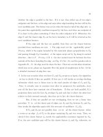
considered in this work is presented in Fig. 1.
Taking into account the type of mobility of their components, there are 4 possible
configurations of mobile manipulators: type
(
)
hh, - both the platform and the manipulator
holonomic, type
(
)
nhh, - a holonomic platform with a nonholonomic manipulator, type
()
nhh, - a nonholonomic platform with a holonomic manipulator, and finally type

()
nhnh,-
both the platform and the manipulator nonholonomic. The balancing robot is a mobile
manipulator of
()
hnh, type because nonholonomic constraints occur only in the motion of
the mobile part (wheels) and the motion of the inverted pendulum (rigid manipulator with
only one degree of freedom) is holonomic.
In the literature it can be found control laws for balancing robot but all solutions to this
problem use either local linearization of the model (Segbot, 2004) or linear controllers (R.
Chi Ooi, 2003). Such linear models and controllers are valid only local, near the desired
configuration and therefore their application is limited only to stabilization of the pendulum
about
0=
d
α
. However, if the fully nonlinear character of the dynamics is explored, then it
is possible to obtain other nonlinear control laws preserving not only point stabilization of
the pendulum but the trajectory tracking, too. In this work a new nonlinear control
algorithm for balancing robot guaranteeing trajectory tracking for the inverted pendulum is
introduced.
This paper is organized as follows. In Section 2 a mathematical model of nonholonomic
balancing robot is obtained. Nonholonomic constraints in the model come from an
assumption about frictionless motion of robot's wheels. In Section 3 control problem is
Automation and Robotics

88
formulated. Section 4 is devoted to the design of nonlinear control algorithm. The proof of
the convergence of this algorithm is included. Section 5 contains simulation results which
illustrate proper working of the proposed nonlinear controller. In Section 6 some

conclusions are presented.


Fig. 1. Balancing robot: inverted pendulum with two fixed wheels on common axis
2. Mathematical model of nonholonomic balancing robot
We consider the mobile manipulator which consists of two subsystems, namely of rigid
manipulator (inverted pendulum) and mobile platform (two fixed wheels located on
common axis – unicycle).
2.1 Nonholonomic constraints
The motion of wheels can be described using generalized coordinates
5
Rq
m
∈
and genera-
lized velocities
5
Rq
m
∈

.
(
)
21
φφθ
yxq
T
m
=

where
()
yx, denote Cartesian coordinates of the center of the axis relative to the basic frame
00
YX ,
θ
is an angle between
p
X and
0
X axis and
i
φ
is a rotation angle of ith wheel. The
mobile subsystem should move without slipping of wheels. This assumption implies the
existence of 3 independent nonholonomic constraints which can be expressed in the so-
called Pfaff’s form

(
)
0
=
mm
qqA

, (1)
Nonlinear Control Law for Nonholonomic Balancing Robot

89

where
(
)
m
qA is a full rank matrix of (3 x 5) size. Due to (1), since the platform velocity is
always in the null space of
A, it is always possible to find a vector of special auxiliary
velocities
m
R∈
η
, 235
=
−
=
m , such that

(
)
η
mm
qGq
=

, (2)
where
(
)
m
qG is an 5 x 2 full rank matrix satisfying

(
)
(
)
0
≡
mm
qGqA .
2.2 Dynamic model of the mobile manipulator of (nh, h) type
Let a vector of generalized coordinates of the mobile manipulator be denoted as
6
R
q
q
m
∈
⎟
⎟
⎠
⎞
⎜
⎜
⎝
⎛
=
α
,
where
5
Rq

m
∈
is a vector of generalized coordinates for the mobile platform and R∈
α

describes an angle between the inverted pendulum (axis X
w
) and vertical direction. Because
of the nonholonomic character of constraints, to obtain the dynamic model of the balancing
robot, the d'Alembert Principle should be used

(
)
(
)
(
)
(
)
(
)
τλ
qBqAqDqqqCqqM
m
+=++

,
. (3)
The model of dynamics (3) can be expressed in more detail as
⎟

⎟
⎠
⎞
⎜
⎜
⎝
⎛
+
⎟
⎟
⎠
⎞
⎜
⎜
⎝
⎛
=
⎟
⎟
⎠
⎞
⎜
⎜
⎝
⎛
+
⎟
⎟
⎠
⎞

⎜
⎜
⎝
⎛
⎥
⎦
⎤
⎢
⎣
⎡
+
⎟
⎟
⎠
⎞
⎜
⎜
⎝
⎛
⎥
⎦
⎤
⎢
⎣
⎡
0
0
0
2221
1211

2221
1211
τ
λ
αα
B
A
D
q
CC
CCq
MM
MM
T
mm





where
()
qM

=
⎥
⎦
⎤
⎢
⎣

⎡
2221
1211
)(
)()(
MqM
qMqM
- inertia matrix,
()
qqC

,
=
⎥
⎦
⎤
⎢
⎣
⎡
0),(
),(),(
21
1211
qqC
qqCqqC


- matrix coming from Coriolis and centrifugal forces,
()
qD

=
⎟
⎟
⎠
⎞
⎜
⎜
⎝
⎛
D
0
- vector of gravity,
3
R∈
λ

- vector of Lagrange multipliers,
()
qB
=
⎥
⎦
⎤
⎢
⎣
⎡
00
0)(
m

qB
- input matrix,
τ

=
⎟
⎟
⎠
⎞
⎜
⎜
⎝
⎛
0
m
τ
- vector of controls.
The model of dynamics (3) of the
(
)
hnh, mobile manipulator is often called a model in
generalized coordinates.
Automation and Robotics

90
Now we want to express the dynamics using auxiliary velocities (2) for the mobile platform.
We compute
(
)
(

)
ηη
mmm
qGqGq



+=

and eliminate from the model (3) the vector of Lagrange multipliers (using the condition
(
)
(
)
0≡
m
T
m
T
qAqG
) by left-sided multiplying the mobile platform equations by
()
m
T
qG

matrix. After substituting for
m
q


and
m
q

we get

(
)
⎟
⎟
⎠
⎞
⎜
⎜
⎝
⎛
=
⎟
⎟
⎠
⎞
⎜
⎜
⎝
⎛
+
⎟
⎟
⎠
⎞

⎜
⎜
⎝
⎛
⎥
⎥
⎦
⎤
⎢
⎢
⎣
⎡
+
+
⎟
⎟
⎠
⎞
⎜
⎜
⎝
⎛
⎥
⎦
⎤
⎢
⎣
⎡
0
0

2221
121111
2221
1211 m
T
TT
TT
BG
D
CGC
CGGMGCG
MGM
MGGMG
τ
α
η
α
η




(4)
We introduce a new symbol covering centrifugal and Coriolis forces as well as gravity. Then
we obtain the model expressed in more compact form as follows

⎟
⎟
⎠
⎞

⎜
⎜
⎝
⎛
=
⎟
⎟
⎠
⎞
⎜
⎜
⎝
⎛
+
⎟
⎟
⎠
⎞
⎜
⎜
⎝
⎛
⎥
⎥
⎦
⎤
⎢
⎢
⎣
⎡

0
*
*
2
*
1
*
22
*
21
*
12
*
11
m
B
F
F
MM
MM
τ
α
η


(5)
where the arguments of matrices and vectors are omitted for the sake of simplicity. We will
refer to the model (5) as the model of dynamics of the
(
)

hnh, mobile manipulator expressed
in auxiliary variables.
2.3 Partial global linearization
The dynamic model of nonholonomic balancing robot can be considered as a mobile
manipulator with one passive degree of freedom (degree of freedom without actuator). The
role of this passive joint plays the inverted pendulum. For such the object it is possible to
introduce due to (De Luca et al., 2001) partial global linearization, which transforms the
model in auxiliary velocities to a form more convenient from control's point of view. For this
reason we extract
α

from the second matrix equation of (5)

(
)
(
)
*
2
*
21
1
*
22
FMM +−=
−
ηα

(6)
and put it into the first equation, (Ratajczak & Tchoń, 2007). Then we get the following

expression

(
)
(
)
m
BqqFqM
τη
*
, =+


, (7)
where
(
)
(
)
(
)
(
)
qMqMqMMqM
*
21
1
*
22
*

12
*
11
−
−=

(
)
(
)
(
)
(
)
qqFqMqMFqqF

,,
*
2
1
*
22
*
12
*
1
−
−=

Now a linearizing control law with a new control input

u should be introduced

(
)
() ()
{
}
qqFuqMB
m

,
1
*
+=
−
τ
(8)
Nonlinear Control Law for Nonholonomic Balancing Robot

91
to get a model (5) defined as a partially linearized control system

(
)( )
⎪
⎩
⎪
⎨
⎧
=

+−=
−
u
FMM
η
ηα


*
2
*
21
1
*
22
(9)
Such a system is a point of departure to design a new nonlinear control algorithm
preserving not only point stabilization but trajectory tracking as well.
3. Control problem statement
In the paper we will find a control law guaranteeing the proper behaviour of the balancing
robot. The task of the robot is to follow the desired trajectory
(
)
t
d
α
(trajectory tracking or
point stabilization) of the inverted pendulum without slipping of platform's wheels.
A goal of this paper will be to address the following control problem for balancing robot
given by the model (9):

Find control law
u such that the balancing robot with the known dynamics follows a
desired trajectory
(
)
t
d
α
without slippage of platform's wheels and tracking errors
converge against zero.
To design a controller for the such the mobile manipulator, it is necessary to observe that
complete nonholonomic system (9) is a cascade with two subsystems. For this reason the
structure of the controller is divided into two parts due to backstepping-like procedure
(Krstić et al., 1995):
1.
kinematic level -
r
η
represents an embedded control input, which ensures the
convergence the real trajectory
α
of the inverted pendulum to the desired trajectory
()
t
d
α
for the equation of constraints (6) if the dynamics were not present,
2.
dynamic level - as a consequence of cascaded structure of the system model, the
pendulum's angle

α
cannot be commanded directly, as is assumed in the design of
control on kinematic level, and instead it must be realized as the output of the partially
linearized dynamics driven by
u. The dynamic input u intends to regulate
η
toward
the embedded control input
r
η
, and therefore, attempts to provide control input
necessary to track the desired trajectory.
Because there exists a difference between the real velocity of the mobile platform
η
and the
embedded control input
r
η
at the start position, it is necessary to account for the influence of
the error
r
e
η
η
η
−= on the behaviour of the full mathematical model of the nonholonomic
balancing robot.
4. Nonlinear control law
4.1 Reference auxiliary velocities
r

η

Let some reference functions describing desired accelerations of platform's wheels will be
defined as follows

(
)
(
)
αα
αη
eKeKFMM
pddr
−−=+−
−


*
2
*
21
1
*
22
, 0, >
pd
KK , (10)
Automation and Robotics

92

where
d
e
α
α
α
−
=

is a tracking error of the inverted pendulum. It is obvious that
r
η
is not unique defined,
because this equation is scalar and
2
R
r
∈
η
. However, it is possible to assume some
relationship between
r1
η
and
r2
η
(for instance
rr 21
ηη
=

) and to get unique solution of (10).
The motion of wheels with velocities
r
η
preserves convergence of the inverted pendulum to
the desired constant configuration
d
α
or to the desired trajectory
(
)
t
d
α
. The main problem is
that the real velocities of wheels
η
are not equal to the reference velocities
r
η
at the
beginning of the motion. It means that some errors occur on the dynamic level and disturb
the behaviour of the balancing robot. Therefore we want to prove using Lyapunov-like
function that the properly chosen control law on dynamic level can guarantee the
asymptotic convergence of these errors to zero. As a consequence we obtain stabilization of
the pendulum about the desired trajectory (or configuration).
4.2 Nonlinear controller
We consider the model of the balancing robot (9) expressed in auxiliary variables. We
assume that we know the solution
r

η
to the constraints equation (10), which preserves a
convergence of real coordinate
)(t
α
of the inverted pendulum to the desired trajectory
()
t
d
α
. Then we propose a new control algorithm guaranteeing asymptotic trajectory
tracking for all coordinates of the mobile manipulator. This control law is defined by
expression

η
η
eKu
mr
−
=

, 0>
m
K (11)

where K
m
is some diagonal regulation matrix and
⎟
⎟

⎠
⎞
⎜
⎜
⎝
⎛
=
⎟
⎟
⎠
⎞
⎜
⎜
⎝
⎛
−
−
=−=
2
1
22
11
η
η
η
ηη
ηη
ηη
e
e

e
r
r
r


is an error appearing on dynamic level, if real velocities of wheels are not equal to reference
velocities, i.e.
()
(
)
00
r
ηη
≠
. In such a situation, on the dynamic level we have the dynamic of
the closed-loop error given by

0
=
+
ηη
eKe
m

(12)

which due to positive definiteness of K
m
matrix is exponentially fast convergent to 0. On the

other side, on kinematic level (the equation describing constraint, i.e. trajectory of a passive
joint) the motion of the inverted pendulum is disturbed in the following way

(
)
(
)
(
)
(
)
ηααη
αηα
eKMeKeKFMeKMM
mpddmr
1
*
22
*
2
1
*
22
*
21
1
*
22
−−−
+−−=−−−=



. (13)