Frontiers in Robotics, Automation and Control Part 2 pot

Towards a Roadmap for Effective Handset Network Test Automation

23
language, such as XML. For example, consider the XML version of the above BNF
description:

TEST-CASE :: = <test-case>
<tc-head > TC-HEAD </tc-head>
<list> <step> STEP </step> </list>
</test-case>
TC-HEAD ::= <tc-head id=”SYMBOL” description=”NAME” estimated-time = “TIME”>
<list> <precondition> PRECONDITION </precondition> </list>
<list> <reference> REFERENCE </reference> </list>
</tc-head>
STEP ::= <step step-number=”NUMBER” technique=“SYMBOL”>
<procedure> PROCEDURE </procedure> </list>
<expected-result> EXPECTED-RESULT </ expected-result >
</step>

Several ontological concepts are represented in such a description. For example, TEXT-
CASE, TC-HEAD and STEP are examples of classes. TC-HEAD has three attributes: id,
description and estimated-time. Finally, the definition structure itself defines the relations
among the classes. For example, TEST-CASEs contain one TC-HEAD and a non empty list of
STEPs. Modern programming languages, like Java, provide a strong support for the
manipulation of XML-based descriptions via, for example, packages to create parsers and
objects that represent the classes and attributes defined in the description. The next section
shows how this kind of description can be used during the test process.

4. Planning the Test Suite

As discussed before, test automation is an appropriate technique to deal with the current

handset test scenario. We have observed that the common approach used in test automation
is to employ pre-defined recorded test cases, which can be created and edited in tools
provided by simulation environments. Such tools also enable the building of different and
more complex tests from previous ones. However, this entire process is carried out
manually. Thus, we have an automatic execution of tests, but using fixed sequences of test
cases, so that the sequence is not automatically adapted to specific scenarios.
The idea explored in this section is to develop a mechanism that autonomously creates test
cases based on devices and environment features. This mechanism must specify the most
appropriate sequence of test cases for a specific handset, also minimizing the total test time.
For that end we have investigated the Artificial Intelligence (AI) Planning technique (Ghallab
et al., 2004), which is used to create optimal sequences of actions to be performed in some
specific situation. One of the advantages of AI planning is its modelling language, which has
a similar syntax to the language used for test case description. Furthermore, the language is
open, providing a direct way to represent states (situations of tests), goals (desired results of
tests) and actions (steps of each test case). This section details these issues, starting with a
brief introduction to AI planning and its fundamentals.
Frontiers in Robotics, Automation and Control

24
4.1 Fundamentals of AI Planning
AI Planning can be viewed as a type of problem solving in which a system (Planner) uses
beliefs about actions and their consequences to search for a solution over a space of plans or
states. The key idea behind planning is its open representation of states (e.g., test case
scenarios), goals (e.g., expected results of test cases) and actions (e.g., steps of a test case).
States and goals are represented by sets of sentences, and actions are represented by logical
descriptions of preconditions and effects. This enables the planner to make direct
connections between states and actions. The classical approach to describe plans is via the
STRIPS language (Fikes & Nilsson, 1971). This language represents states by conjunctions of
predicates applied to constant symbols. For example, we can have the following predicates
to indicate the initial state of a handset network: FreqRange(cell

a
,900) ∧
FreqRange(cell
b
,1800). Goals are also described by conjunctions of predicates, however they
can contain variables rather than only constants. Actions, also called operators, consist of
three components: action descriptions, conditions and effects. Conditions are the (partial)
mandatory states to the application of the operator and effects are the (partial) final state
after its application. Using these basic definitions, the representation of plans can be
specified as a data structure consisting of the following four elements (Wilkins, 1994):
• A set of plan steps, each of them representing one of the operators;
• A set of tasks ordering constraints. Each ordering constraint is of the form S
i
» S
j
, which is
read as “S
i
before S
j
” and means that step S
i
must occur sometime before step S
j
;
• A set of variable binding constraints. Each variable constraint is of the form v = x, where v
is a variable in some task and x is either a constraint or another variable; and
• A set of causal links. A causal link is written as {T
i
→T

j
}
c
and read as “Ti achieves c for T
j
”.
Causal links serve to record the purpose(s) of steps in the plan. In this description, a
purpose of T
i
is to achieve the precondition c of T
j
.
Using these elements, we can apply a Partial-Order Planning (POP) algorithm, which is able
to search through the space of plans to find one that is guaranteed to succeed. More details
about the algorithm are given later.

4.2 Test Case as Planning Operators
Let us consider now the process of mapping a test case to a planning method. One of the
parts of this research is to codify each of the user cases in a plan operator. As discussed
before, a plan operator has three components: the action description, the conditions and the
effects. Therefore we need to find information inside user tests to create each of these
components. Starting by the action description, this component is just a simple and short
identifier that does not play any active role during the decision process of the planner. For
its representation we are issuing identifiers that relate each action description with a unique
test case TC. Second, we need to specify the operator conditions. The test case definition has
an attribute called precondition that brings exactly the semantic that we intend to use for
operator conditions. Note, however, that this description is a natural language sentence that
must be translated to a logic predicate before being used by the planner. Finally, the effects
do not have a direct mapping from some component of the test case descriptor. However,
each step of the test case (e.g., Table 1) is one action that can change the current state of the

domain. Consequently, the effects can be defined by the conjunction of the expected results
of each step, if this step has the feature of changing the domain status. Another observation
is that sequential steps can change a given status. Thus, only the last change of a status must
Towards a Roadmap for Effective Handset Network Test Automation

25
be considered as an effect. As discussed for preconditions, this conjunction of plan steps
results also must be codified in logic predicates.

Step Procedure Expected result
01
Switch handset on.
“G-Cell B MS->SS RACH CHANNEL REQUEST”
02 Set the LOCATION UPDATE to
cell B.
“G-Cell B SS->MS SDCCH/4 LOCATION
UPDATING ACCEPT”
03 Make a voice call.
“G-Cell B SS->MS SDCCH/4 CALL PROCEEDING”
04 Execute HANDOVER to the cell A.
“G-Cell B SS->MS FACCH CALL CONNECT”
05 Execute HANDOVER to the cell A.
“G-Cell A SS <- MS FACCH HANDOVER
COMPLETE”
06 Deactivate voice call.
“G-Cell A MS->SS FACCH DISCONNECT”
07 Deactivate the handset.
“G-Cell A MS->SS SDCCH/4 IMSI DETACH
INDICATION”
08 Deactivate cells and B.

“Verdict : PASS”
Table 1. Partial specification of a test case.

A close investigation into the test cases shows that they are not dealing with operations
related to changes in some of the network domain parameters, such as frequency band or
number of transceivers in each cell. To have a complete automation of the handsets’ network
tests, the planner needs special operators that are able to change such parameters.
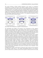
Considering this fact, the set of automation operators can be classified into two groups: the
Test Case Operators (TCO) and the Domain Modify Operators (DMO). The use of both
operators is exemplified in the figure below (Fig. 5).












Fig. 5. Test case for a handover between two cells of 1800 MHz.

During the planning process, a planner should normally consider all the test case operators
(TCO) of a scenario S
1
before applying a DMO and change to S
2
. Actually the number of

changes between scenarios (or use of DMO’s) can be a measure of the planner performance.
Test
Begin
T
1
Test
End
T
2
T
3
T
4
T
5
T
6
DMO
TCO
TCO
TCO
TCO
TCO
TCO
S
1

S
2

Frontiers in Robotics, Automation and Control

26
A complete test case plan is a sequence of these operators in which every precondition, of
every operator, is achieved by some other operator.

4.3 Planning Algorithm
The reasoning method investigated during this project is described via a Partial-Order
Planning (POP) algorithm (Nguyen & Kambhampati, 2001). A POP planner has the ability of
representing plans in which some steps are ordered with respect to each other while other
steps are unordered. This is possible because they implement the principle of least
commitment (Weld, 1994), which says that one should only make choices about things that
it currently cares about, leaving the other choices to be worked out later.
The pseudocode below (1 to 4) describes the concept of a POP algorithm, showing how it
can be applied to the handsets‘ network test domain. This pseudocode was adapted from
the original POP algorithm (Russel & P. Norvig, 2002).

function POP(testBegint,testEnd,operators) return plan
plan ← Make-Basic-Plan(testStart, testFinish)
loop do
if Solution?(plan) then return plan
T
i
, c ← SELECT-SUBGOAL(plan)
CHOOSE-OPERATOR(plan,operators, T
i,
c)
RESOLVE-THREATS(plan)
end

(1)

Code (1) shows that the POP is a loop that must create a plan from a testBegin state (no tests
performed) to a testEnd state (all tests performed). For that end, the loop extends the plan by
achieving a precondition c of a test case T
i
, which was selected as a subgoal of plan.
Code (2) accounts for the selections of this subgoal:

function SELECT-SUBGOAL(plan) returns T
i,
c
pick a test stateT
i
from TEST_STEPS(plan)
with a precondition c that has not been achieved
return step T
i
,c

(2)

Code (3) details the choice of an operator T
add
(TCO or DMO), which achieves c, either from
the existing steps of the plan or from the pool of operators. Note that the causal link for c is
recorded together with an ordering constraint. If T
add

is not in TEST_STEPS (T
i
), it needs to
be added to this collection.
We can improve the SELECT-SUBGOAL function by adding a heuristic to lead the choice of
a test goal. During the test process, if one of the tests fails, the problem must be fixed and all
the test collection carried out again. Imagine an extreme scenario where a problem is
detected in the last test. In this case, the test process will take about twice the normal time to
be performed if any other problem is found. Considering this fact, the SELECT-SUBGOAL
function could identify and keep track of the tests where errors are more commons. This
could be implemented via a module of learning (Langley & Allen, 1993), for example. Based
Towards a Roadmap for Effective Handset Network Test Automation

27
on this knowledge, the function should give preference to tests with a bigger probability to
fail because then the test process will be interrupted earlier.

procedure CHOOSE-OPERATOR(plan,operators, T
i,
c)
choose a step T
add
from operators or TEST_STEPS (plan) that has c as an effect
if there is no such step then fail
add the causal link {T
add
→ T
i
}
c

to LINKS(plan)
add ordering constraint T
add
» T
i
to ORDERINGS(plan)
if T
add
is a newly added step from operators then
add T
add
to TEST_STEPS (T
i
)
add Start » T
add
» Finnish to ORDERINGS(plan)
end




(3)

The last procedure, Code (4), accounts for resolving any threats to causal links. The new
step T
add
may threaten an existing causal link or an existing step may threaten the new
causal link. If at any point the algorithm fails to find a relevant operator or fails to resolve a
threat, it backtracks to a previous choice point.

procedure RESOLVE-THREATS(plan)
for each T
threat
that threatens a link {T
i
→T
j
}
c
in LINKS(plan) do
choose either
Promotion: Add S
threat
» S
i
to ORDERINGS(plan)
Demotion: Add S
j
» S
threat
to ORDERINGS(plan)
if not CONSISTENT(plan) then fail
end


(4)

POP implements a regression approach. This means that it starts with all the handset

network tests that need to be achieved and works backwards to find a sequence of operators
that will achieve them. In our domain, the final state “Test_End” will have a condition in
the form: Done(TC
1
) ∧ Done(TC
2
) ∧ … ∧ Done(TC
n
), where n is the total number of test cases
(TC). Thus, the “Test_Begin” has a effect in the form: ¬Done(TC
1
) ∧ ¬Done(TC
2
) ∧ … ∧
¬Done(TC
n
). In this way, all TCOs must have an effect in the form Done(TC
i
), where i is an
integer between 1 and n. The other effects of each TCO change the current plan state,
restricting the operations that can be used. If there is a fail, this could indicate that a DMO
must be applied to change the scenario (network parameters).
According to [VanBrunt, 1993], the test methodology to handset network, which is based on
GSM, are focused on conformance evaluations used to validate the underlying components
of the air interface technology. However, the launch of new technologies, such as the
WCDMA (Wideband Code Division Multiple Access), could change the current way that tests
are performed, requiring, for example, a more progressive and integrated approach to
evaluation of user equipments. Considering this fact, features like maintenance and
extensibility must be considered during the development of test automation. In our
approach, any new requirement can be easily contemplated via the creation of new

operators. New network configurations could also be defined via the definition of new
scenarios and DMOs that change the conditions of test applications.
Frontiers in Robotics, Automation and Control

28
5. Automation and Autonomic Architectures and Autonomic Computing

Automation test architectures intend to support the execution of tests by computational
processes, independently from human interference. This automation considers a pre-defined
and correct execution, so that concepts such as adaptation and self-correction are not
generally contemplated. The second and more complex level of automation is characterised
by systems that present some level of autonomy to take decisions by themselves. This kind
of autonomic computing brings several advantages when compared with traditional
automation and several approaches can be employed to implement its fundaments. All
these issues are detailed in this section.

5.1 The CInMobile Automation Tool
We have implemented an automation environment by means of CInMobile (Conformance
Instrument for Mobiles). This tool aims to improve the efficiency of the test process that is
being carried out over the network simulation environment. The CInMobile architecture is
illustrated in follow (Fig. 6), where its main components and their communication are
presented. As discussed before (see Fig. 4), simulator scripts can have prompt commands
that request some intervention from human testers. The first step of our approach was to
lead such commands to the serial port so that they could be captured by an external process
called Handset Automator (HA), running in a second computer. In this way, the HA receives
prompt commands, as operations requests, and analyzes the string content to generate an
appropriate operation, which is sent to the handset in evaluation. The HA can use pre-
defined scripts from the Handset Script Base during this operation. The HA also accounts for
sending synchronization messages to the SAS software, indicating that the requested
handset operation was already carried out.

Fig. 6. CinMobile Architecture.

Both SAS and HA generate logs of the test process. However, results of several handset
operations, over the simulated wireless network, can be identified via comparisons of
resulting handset screens to reference images. Our architecture also supports this kind of
evaluation and its results are considered together with the SAS and HA logs. In fact, each of
these results (images comparison, SAS and HA logs) brings a different kind of information
that must be analyzed to provide useful information about a particular test case.
Towards a Roadmap for Effective Handset Network Test Automation

29
One of the functions of the Automation Controller (AC) process is to consolidate all the test
process resulting information, performing a unified analysis so that a unique final report can
be generated (Fig. 7). The advantage of this approach is that we are passing the
responsibility of reporting the test results from the human testers to an automatic process.
Furthermore, the Final Report Generator (see Fig. 7) can be used to customize the final report
appearance (e.g., using templates) according to user needs.


Fig. 7. Test report generation process.

A second important AC function is associated with the control of script loading in simulator.
This is useful, for example, because some of the tests must be repeated several times and
there is an associated approval percentage. For instance, consider that each test is
represented by the 3-tuple <t,η,ϕ>, where t is the test identifier, η is the number of test
repetitions for each device, and ϕ is the approval percentage. Then a 3-tuple specified as
<t
1

,12,75%> means that the t
1
must be performed 12 times and the device will only be
approved if the result is correct at least in 9 of them. However, if the 9 first tests are correct,
then the other 3 do not need to be executed, avoiding waste of time.
A last AC core function is to manage the performance of several handsets automators. Some
tests cases, mainly found in the Bluetooth battery, require the use of two of more handsets to
evaluate, for example, operations of voice conference (several handsets sharing the same
Voice Traffic Channel) over the network. In this scenario, the AC accounts for the tasks of
synchronization, among simulator and handset automators, and consolidation of multiple
handset logs during the generation of test reports.

5.2 Autonomic Computing
The test process, carried out by our Test Center team, currently provides a percentage of
about 53% of automation. However the level of automation provided to such tests is not
enough to support a total autonomic execution, that is, without the presence of human testers.
Considering this fact, our aim is to implement new methods that enable a total autonomic
execution, so that tests can be executed at night, for example, increasing the use time of the
simulation environment per day and, consequently, decreasing the total test time and
operational cost. Our fist experiment was carried out with the E-mail battery. This battery
was chosen because it is currently 100% automatic and represents about nine hours of test
time. Thus, we could decrease in about one day the test process if such a battery could be
performed at night. These new sets of tests, that can run without the human presence, we
call autonomic tests.
Frontiers in Robotics, Automation and Control

30
The study of autonomic computing was mainly leaded by IBM Research and a clear
definition is (Ganek & Corbi2003): “Autonomic computing is the ability of systems to be
more self-managing. The term autonomic comes from the autonomic nervous system, which

controls many organs and muscles in the human body. Usually, we are unaware of its
workings because it functions in an involuntary, reflexive manner for example, we do not
notice when our heart beats faster or our blood vessels change size in response to
temperature, posture, food intake, stressful experiences and other changes to which we're
exposed. And, by the way, our autonomic nervous system is always working“.
An autonomic computing paradigm must have a mechanism whereby changes in its
essential variables can trigger changes in the behavior of the computing system such that the
system is brought back into equilibrium with respect to the environment. This state of stable
equilibrium is a necessary condition for the survivability of a system. We can think of
survivability as the system’s ability to protect itself, recover from faults, reconfigure as
required by changes in the environment, and always to maintain its operations at a near
optimal performance. Its equilibrium is impacted by both the internal and external
environment.
An autonomic computing system (Fig. 8) requires: (a) sensor channels to sense the changes
in the internal and external environment, and (b) return channels to react to and counter the
effects of the changes in the environment by changing the system and maintaining
equilibrium. The changes sensed by the sensor channels have to be analyzed to determine if
any of the essential variables has gone out of their viability limits. If so, it has to trigger some
kind of planning to determine what changes to inject into the current behavior of the system
such that it returns to the equilibrium state within the new environment. This planning
would require knowledge to select the right behavior from a large set of possible behaviors
to counter the change. Finally, the manager, via return channels, executes the selected
change. Thus, we can undersdand the operation of an aunomic system as a continuous cycle
of sensing, analyzing, planning, and executing; all of these processes supported by
knowledge (Kephart & Chess, 2003).


Fig. 8 – The classical autonomic computing architecture.

This classical autonomic architecture (Fig. 8) acts in accordance with high-level policies and

it is aimed at supporting the principles that govern all such systems. Such principles have
been summarized as eight defining characteristics (Hariri et al, 2006):
Towards a Roadmap for Effective Handset Network Test Automation

31
• Self-Awareness: an autonomic system knows itself and is aware of its state and its
behaviour;
• Self-Protecting: an autonomic system is equally prone to attacks and hence it should be
capable of detecting and protecting its resources from both internal and external attack
and maintaining overall system security and integrity;
• Self-Optimizing: an autonomic system should be able to detect performance degradation
in system behaviour and intelligently perform self-optimization functions;
• Self-Healing: an autonomic system must be aware of potential problems and should have
the ability to reconfigure itself to continue to function smoothly;
• Self-Configuring: an autonomic system must have the ability to dynamically adjust its
resources based on its state and the state of its execution environment;
• Contextually Aware: an autonomic system must be aware of its execution environment
and be able to react to changes in the environment;
• Open: an autonomic system must be portable across multiple hardware and software
architectures, and consequently it must be built on standard and open protocols and
interfaces;
• Anticipatory: an autonomic system must be able to anticipate, to the extent that it can, its
needs and behaviours and those of its context, and to be able to manage itself proactively.
An autonomic manager component does not need to implement all these principles and the
choice for one or more depends on the kind of managed element that we are working with.
For example, the implementation of the Self-Protecting principle only makes sense if we are
working with systems that require a high level of security, such as Internet or network
systems. In our case, in particular, we are initially focusing our investigation on three of
these principles: Self-Awareness, Self-Healing and Contextual Awareness.
We can find several similarities if we compare the classical autonomic computing

architecture to the structure (Fig. 9) of an intelligent utility-based agent (Russel & Norvig,
2002). First, both systems present specific components to sense (sensors channels) the
environment (or managed element) and to execute operations (return channels) on such an
environment. Second, the knowledge of autonomic computing architectures can be
compared to the knowledge of agents (knowledge about its state, how the world evolves,
what its actions do and utility of decisions). Finally, in both cases, such knowledge supports
the process of analysis and planning of actions, which are going to be executed on the
environment.


Fig. 9. Utility-based agent structure.
Frontiers in Robotics, Automation and Control

32
The autonomic manager module, which is in development by our team, is based on this
agent approach. For that end, we are specifying the five components of the autonomic
architecture (monitor, knowledge base, analyzer, planner and executor) in the following
way:
• Monitor – this component is a listener of exceptional events (e.g., Java exceptions),
variable content updating (e.g., serial port identifiers) and temporal references (when
specific no-exceptional start events are flagged, a timer is started to check if such events
finish within pre-defined intervals) ;
• Knowledge base – set of objects that represent both a collection of facts and rules. Facts
abstract the current status of the managed element, whereas rules mainly indicate what
the systems must do if some event is flagged;
• Analyzer – events received by the monitor need to be analysed in a holistic way. This
means, rather than analysing some event individually, we must perform such analysis
considering the current status of the knowledge base. For this analysis we use a set of
analysis rules, which are part of the knowledge base;
• Planner – analysis rules insert new facts into the knowledge basis, which are used by the

planner to decide the actions that are going to be performed. The planner is in fact a set of
rules, which we call decision rules;
• Executor – this component has a set of methods that are able to modify the state of the
managed element. This set of methods is limited and must be predefined, according to a
previous study of the system.
The knowledge base, analyzer and planner are being specified as a production system and
for that we are using JEOPS - Java Embedded Object Production System (Filho & Ramalho,
2000). The main reason for its use is its first-order forward-chaining inference approach,
which starts with the available facts and uses inference rules to extract more facts until an
appropriate action is reached. Another reason is its complete integration with Java, which is
used in the development of our software. Such components together provide the
mechanisms to support the principles of Self-Awareness (knowledge base represents an
internal state and updates it), Self-Healing (rules identify problems and trigger recovering
methods) and Context Awareness (rules consider the current context once events are
analysed in a holistic way).

6. Automation Monitoring and Control via DMAIC Concepts

This section discusses the use of DMAIC (Define, Measure, Analyze, Improve, and Control)
(Simon, 2007), a Six Sigma (Harry, 1998) framework based on measures and statistical
analysis, which has commonly been applied during several stages of software development
(Biehl, 2004). We show that, using DMAIC, we could be able to both find out automation
process failures and identify potential points in a test process that require a review.
Furthermore, we could monitor the quality of the test process, as discussed below.

6.1 Six Sigma and DMAIC Concepts
Six Sigma is a set of practices to systematically improve processes by eliminating its defects.
For that, Six Sigma stresses two main points: processes can always be measured, analyzed,
improved and controlled; and continuous efforts to reduce variation in process outputs are
essential to business success.

Towards a Roadmap for Effective Handset Network Test Automation

33
In this discussion we are interested in the statistical fundaments of Six Sigma. In fact, one of
the features of its frameworks is the use of measurements and statistical analysis. However,
it is a mistake to view the core of Six Sigma frameworks as statistics; an acceptable Six Sigma
project can be started with only rudimentary statistical tools. The Six Sigma idea is very
similar to SPC (Statistical Process Control) analysis (Florac & Carleton, 1999), which
identifies both the location of problems (producing defectives) and whether or not you can
cost-effectively fix them.
Six Sigma provides two main frameworks, which can be better applied according to the
scenario that we have. Such scenarios are: (1) there is no process at all (note that a bad
process is as good as no process); and (2) there is already existing process(es) that is working
reasonably well. In the first scenario, whose focus is on process design, Six Sigma suggests
the use of the DMADV framework. DMADV is summarized by the following ideas:

• Define the project goals and customer (internal and external) deliverables;
• Measure and determine customer needs and specifications;
• Analyze the process options to meet the customer needs;
• Design (detailed) the process to meet the customer needs;
• Verify the design performance and ability to meet customer needs.
In the second scenario, whose focus is on significant process improvements, Six Sigma
suggests the use of the DMAIC framework. DMAIC stands for:
• Define process goals in terms of key critical parameters (i.e. critical to quality or critical
to production) on the basis of customer requirements;
• Measure the current process performance in context of goals;
• Analyze the current scenario in terms of causes of variations and defects;
• Improve the process by systematically reducing variation and eliminating defects;
• Control future performance of the process.
Sometimes a DMAIC application may turn into a DMADV application because the process

in question requires complete re-design to bring about the desired degree of improvement.
Such a discovery usually occurs during the improvement phase of DMAIC. In our case we
have decided for DMAIC because we already have a process and our intention is the
improvement of this process and detection of its problems.

6.2 DMAIC Phases Application
As discussed before, Six Sigma specifies more than one problem-solving framework, as
processes and situations can vary on their nature. We have decided for DMAIC because it is
more appropriate for existing processes. In this way, this section summarizes the role of
each DMAIC phase and details how we have specified each of these phases to work during
the measure and analysis of our test process.

Define Phase

The main role of the Define phase is to formally specify the DMAIC project, its elements,
context, importance and purpose. For our test process, in particular, the most relevant
output from this phase is the definition of what is the issue that we intend to improve. This
issue is the prediction of total test time or test effort for a handset.
To better understand this problem, consider a partial list of handset features (MMS,
Bluetooth, EDGE, etc.). Each handset that is going to be evaluated supports a subset of such
Frontiers in Robotics, Automation and Control

34
features, which are used to compose its test suite. For example, if a handset does not support
Streaming, all the tests related to this features are removed from the evaluation set. Thus, we
can conclude that the total test time is not the same for all handset models.
When the development unit sends a handset to our test team, they need to know the total
test time so that they can plan their next actions. To deal with unpredictable problems, we
can add an error limit to our estimations. For example, if we estimate that a battery is
performed in 120 minutes, we can add 20% of error and say that it performs in 144 minutes.

This approach can generate delays in the development unit process and, consequently, in
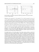
the process as a whole. To exemplify the problem of simple estimations, i.e. estimations
without a real statistical investigation, observe the graph below (Fig. 10) where the Y-axis
represents time and X-axis represent the test batteries. This graph represents the results of
our first evaluation running and it brings information about the estimated time for each test
battery and the real time of its execution
2
.


Fig 10. Relation between estimated and execution time.

All our estimates were too high and in some cases (e.g., MM - Multimedia Messaging Service -
and WP – Wireless Application Protocol) the estimates were very deficient. All these
estimation problems raise collateral effects to the development unit, which could have
defined a better operational plan if they had more effective test time estimates.

Measure Phase


The most important output of the Measure phase is the Baseline, a historical measurement of
indicators chosen to determine the performance before changes made by the DMAIC

2
Zero Execution time means that the related battery was not applied to the handset in test (e.g., ST – Streaming).
Towards a Roadmap for Effective Handset Network Test Automation

35
application. These indicators are also measured to assess the progress during the Improve
phase and to ensure that such an improvement is kept after the Control phase. The lead

indicator, in our case the prediction of the total test time, is used to track variables that affect
its value. Our investigation in this phase is separately performed on each test battery, so
that we can perform a more granular investigation on the results. This approach is justified
because the batteries have very particular features, which can be better identified and
understood if they are analysed in this way. For simplifications, let us consider that there
exists only one battery and the total test time is the time to perform this battery. Considering
this premise, The Shewhart Graph (Florac & Carleton, 1999) (Fig. 12) shows the results related
to initial test executions, which were manually carried out in the simulator environment.


Fig. 12. Shewhart Graph for total time of test runs.

The Shewhart graph contains a Central Line (CL), a Lower Control Line (LCL), an Upper
Control Line (UCL) and values related to the issue that we intend to control or improve. In
our case, these values are related to the total test time of initial test runs. These data is
sequentially plotted along the time, so that we have a historical registry of this information.
This is a continuous process and the more data we have, the better will be our Baseline. The
CL represents a central value or average of the measures performed on the issue. Both
control limits, which are estimates of the process bounds based on measures of the issue
values, indicate the limits to separate and identify exceptional points (Humphrey, 1988). The
control limits are placed at a distance of 3-sigma (or 3σ) from the central line (sigma σ is the
standard deviation).
This graph is an appropriate resource to clarify our objectives in using DMAIC. These
objectives and their relation with the graph are:
• More accurate prediction of total test time: this is indicated by the distance between LCL
and UCL. The shorter this distance is, the more accurate our prediction will be;
Frontiers in Robotics, Automation and Control

36
• Test process improvement: the central line (CL) represents our current prevision for the

performance of a test run, considering the complete set of test batteries. Test process
improvements mean to reduce such a prevision. Our goal is indicated by the red bound
line in the graph (goal line);
• Better control: if all total test times are between the control limits, then the test presents
only common causes of variation and we can say that the test is in a statistically
controlled state (stable test). Differently, if a total test time is out of the control limits, the
test presents special causes of variation and we can say that the test is out of statistical
control (unstable test).
Before continuing to the next phase, it is important to understand the meaning of common
and special causes of variation. Common causes of variation are problems inherent in the
system itself. They are always present and affect the output of the process. Examples are
poor training and inappropriate production methods. Special causes of variation are
problems that arise in a periodic fashion and they are somewhat unpredictable. Examples of
special causes are operator error and broken tools. This type of variation is not critical and
only represents a small fraction of the variation found in a process (Deming, 1975).

Analysis Phase


The Analysis phase accounts for raising and validating main causes of problems during the
handsets network test process. Table 2 summarizes examples of such problems for our
domain.

# Cause ( I ) ( C ) ( P )
1 New testers/operators L M L
2 Operational errors H L H
3 Later found incompatibilities M L M
4 Infra-structure support M H M
5 Bugs in network simulator H H L
6 Test version no longer compatible M L H

Table 2. Summary of problems for the handset test domain

Three parameters are associated with each cause of problems: influence on lead indicator (I),
theoretical cost to fix this cause (C), and priority to apply some solution (P). These
parameters can assume three qualitative values: low (L), medium (M) and high (H). Such
values were set based on our first test experiments and discussions with the technical team.
For example, for the first cause we have concluded that the insertion of new testers
(externals and trainers) has a low impact on the test process, despite the fact that they only
have an initial experience in this process. The cost to carry out a special training is medium,
once that we need to allocate a tester engineer to this task. Thus this task is not a priority.
Towards a Roadmap for Effective Handset Network Test Automation

37
Improve Phase


The Improve phase accounts for selecting and implementing solutions to reduce or
eliminate the causes of problems discovered during the Analysis phase. During the Analysis
phase, we have already started the discussion about potential solutions for these causes. The
following actions are examples of solution that could be implemented in our process:
specification of a more granular and formal test process, which focuses mainly on avoiding
loss of data (e.g., extensive use of backups) and finding the points where we can carry out
tasks in parallel to eliminate dependences and producer-consumer like errors. Solutions are
not fixed and they must be adapted to new causes that may appear. This is also one of the
reasons to monitor the process even after the application of solutions.

Control Phase


The Control Phase accounts for maintaining the improvement after each new cycle. In our

case, this cycle represents the execution of a complete test run. This phase is also related to
the process of monitoring the execution of each test, so that new problems can be detected.
According to DMAIC, a new problem is raised when the lead indicator, in our case the total
test time, is out of the control limits. The graph below (Fig. 13) shows an example of new
limit controls that could appear after the application of some solutions. We can observe that
the central line is not reached. However we can see some improvement in terms of a new
central line (shorter total test time) and narrower control limits. From now on, all the
measures must respect such limits.


Fig. 13. New values after the application of solutions

Our test suit is not complete. Currently we are executing 60% of the total number of tests,
already specified by our telecom test team. Furthermore, the evolution of new technologies,
such as 3G, will certainly bring the need for new test cases. All these facts also contribute to
a continuous and dynamic change of the indicator values, which can be monitored via the
use of statistic methods such as the ones used in this work.
Frontiers in Robotics, Automation and Control

38
6. Test Management Tools

A last point to be discussed in this chapter is the use of test management tools as an
alternative to complete some functions required by an automation test architecture. Current
tools
3
can provide one or more from the following features:
• Specification for plans of tests - considers definition of test cases to be applied, test
priority, test strategies, test schedule and resources to be allocated;
• Test evaluation support - considers specification and customization of test evaluation

documents and summary of tests (test results, test cases coverage, process test
environment);
• Extraction of statistical indicators - considers the capture of statistical indicators,
specification and customization of statistical reports;
• Test cases creation - considers the edition and maintenance of test cases;
• Integration support - considers the existence of an API to enable the integration of a tool
platform with external applications;
We can observe that several of these features are already considered by our proprietary
solution. For example, the specification for test plans is covered by the test suit planner
(Section 4). The main advantage in using external test management tools is the quality
provided by several existing commercial systems. However, we must consider if such
systems are flexible enough so that we can make adaptations and customizations in some of
their functions.

7. Conclusion

The purpose of this chapter was to discuss several aspects related to the process of test
automation. With this objective, we have introduced our domain and initial simulation test
environment. Using this environment we have discussed several solutions and concepts that
are currently under investigation by our research team. Furthermore, we have also
discussed a statistical technique for controlling the process during its continuous evolution.

8. Acknowledgements

The authors would like to thank all the test engineers (Amanda Araujo, Karine Santos,
Rivaldo Oliveira and Paulo Costa), software engineers (Angela Freitas and Kleber Carneiro),
telecom internals (Anniele Costa and Ronaldo Bitu) and product manager (Fernando
Buononato) of the CIn/SIDI-Samsung Test Center, which provided the technical details
about the handsets’ network test domain, simulation environment and GSM principles. The
team is also very grateful for the support received from Samsung/SIDI team, in particular

from Ariston Carvalho, Miguel Lizarraga, Ildeu Fantini and Vera Bier. The National Council
for Scientific and Technological Development (CNPq) has provided valuable support to the
project through the Brazilian Federal Law no. 8010/90.
UFPE and Samsung are authorized to reproduce and distribute reprints and on-line copies
for their purposes notwithstanding any copyright annotation hereon. The views and

3
TestLink (), QATraq (), RHT (
rth/), Salome-TMF ( and so on.
Towards a Roadmap for Effective Handset Network Test Automation

39
conclusions contained herein are those of the authors and should not be interpreted as
necessarily representing the official policies or endorsements, either expressed or implied, of
other parties.

8. References

Anite (1999). SAS 12447D/UMOOI GSM-9OO/DCSI800 /PCS-1900. Stand Alone Simulator
User Manual, Rel. 3.0, Anite Telecoms Ltd, Fleet, Hampshire, UK.
Biehl, R. (2004). Six Sigma for Software, IEEE Software, 21, 2, 68-70, USA.
Deming, W. (1975). On probability as a basis for action, The American Statistician, 29, 4, 146-
152.
De Vriendt, J. ; Laine, P. ; Lerouge, C. & Xiaofeng, X. (2002). Mobile network evolution: a
revolution on the move, IEEE Communications Magazine, 40(4):104-111.
Fikes, R. & Nilsson, N. (1971). STRIPS: A New Approach to the Application of Theorem
Proving to Problem Solving, Proceedings of Second International Joint Conference in
Artificial Intelligence, London, UK.
Filho, C & Ramalho, G. (2000). JEOPS – The Java Embedded Object Production System,
Springer Verlag's Lecture Notes in Artificial Intelligence, 1952, 52-61, Heidelberg

Germany.
Florac, W. & Carleton, A. (1999). Measuring the software process: statistical process control
for software process improvement. The SEI Series in Software Engineering, Addison-
Wesley.
Ganek, A. & Corbi, C. (2003). The Dawning of the autonomic computing era, IBM Systems
Journal, 42, 1, 5-18.
Garg, V. (2001). Wireless Network Evolution 2G to 3G. Prentice Hall, 0-13028-077-1, USA.
Ghallab, M.; Nau, D. & Traverso, P. (2004). Automated Planning: theory and practice, Morgan
Kaufmann Publishers, 1-55860-856-7, USA.
Gruber, R. (1995). Toward Principles for the Design of Ontologies Used for Knowledge
Sharing. International Journal Human-Computer Studies, 43, 5/6, 907-928.
Guarino, N. (1995). Formal Ontology, Conceptual Analysis and Knowledge Representation,
International Journal of Human-Computer Studies, 43, 5/6, 625–640.
Hariri, S. et al. (2006). The Autonomic Computing Paradigm, Cluster Computing: The Journal
of Networks, Software Tools, and Applications, 9, 1, 5-17, Kluwer Academic Publishers.
Harry, M. (1998). Six Sigma: A Breakthrough Strategy for Profitability, Quality Progress
Publications, 31, 5, 60-64.
Humphrey, W. (1988). Characterizing the Software Process: A Maturity Framework. IEEE
Software, 5, 2, 73-79.
Kephart, J. & Chess, D. (2003). The Vision of Autonomic Computing, IEEE Computer, 36, 1,
41-50.
Langley, P. & Allen, J. (1993). A unified framework for planning and learning. In S. Minton
(Ed.), Machine learning methods for planning. San Mateo, CA: Morgan Kaufmann.
Nguyen, X. & Kambhampati, S. (2001). Reviving partial order planning, Proceedings of
Seventeenth International Joint Conference in Artificial Intelligence, 459-466, Seattle,
WA, USA.
Russel, S. & Norvig, P. (2002). Artificial Intelligence: A Modern Approach, 2nd Edition,
Prentice Hall, 0-13790-395-2, USA.
Frontiers in Robotics, Automation and Control

40
Rahnema, M. (1993). Overview of the GSM system and protocol architecture, IEEE
Communications Magazine, 42, 4, 493-502.
Simon, K. (2007). DMAIC versus DMADV, Six Sigma WebPage. Available in:
tent/c001211a.asp
VanBrunt, R. (2003). WCDMA versus GSM: handset performance testing, RF Design, 26, 9,
14-23, Cardiff Publishing Company Inc, USA.
Weld, D. (1994). An introduction to least-commitment planning, AI Magazine, 15, 4, 27-61.
Wilkins, D. (1984). Domain-independent planning: representation and plan generation,
Artificial Intelligence, 11, 3, 269- 301.

3

Automatic Speaker Recognition
by Speech Signal

Milan Sigmund
Brno University of Technology
Czech Republic

1. Introduction

Acoustical communication is one of the fundamental prerequisites for the existence of
human society. Textual language has become extremely important in modern life, but
speech has dimensions of richness that text cannot approximate. From speech alone, fairly
accurate guesses can be made as to whether the speaker is male or female, adult or child. In
addition, experts can extract from speech information regarding e.g. the speaker’s state of
mind. As computer power increased and knowledge about speech signals improved,
research of speech processing became aimed at automated systems for many purposes.
Speaker recognition is the complement of speech recognition. Both techniques use similar

methods of speech signal processing. In automatic speech recognition, the speech processing
approach tries to extract linguistic information from the speech signal to the exclusion of
personal information. Conversely, speaker recognition is focused on the characteristics
unique to the individual, disregarding the current word spoken. The uniqueness of an
individual’s voice is a consequence of both the physical features of the person vocal tract
and the person mental ability to control the muscles in the vocal tract. An ideal speaker
recognition system would use only physical features to characterize speakers, since these
features cannot be easily changed. However, it is obvious that the physical features as vocal
tract dimensions of an unknown speaker cannot be simply measured. Thus, numerical
values for physical features or parameters would have to be derived from digital signal
processing parameters extracted from the speech signal. Suppose that vocal tracts could be
effectively represented by 10 independent physical features, with each feature taking on one
of 10 discrete values. In this case, 10
10
individuals in the population (i.e., 10 billion) could be
distinguished whereas today’s world population amounts to approximately 7 billion
individuals.
People can reliably identify familiar voices. About 2-3 seconds of speech is sufficient to
identify a voice, although performance decreases for unfamiliar voices. One review of
human speaker recognition (Lancker et al., 1985) notes that many studies of 8-10 speakers
(work colleagues) yield in excess of 97% accuracy if a sentence or more of the test speech is
heard. Performance falls to about 54% when duration is shorter than 1 second and/or
distorted e.g., severely highpass or lowpass filtered. Performance also falls significantly if
training and test utterances are processed through different transmission systems. A study
Frontiers in Robotics, Automation and Control

42
using voices of 45 famous people in 2 seconds test utterances found only 27% recognition in
an open-choice test, but 70% recognition if listeners could select from six choices (Lancker et
al., 1985). If the utterances were increased to 4 seconds, but played backward (which distorts

timing and articulatory cues), the accuracy resulted to 57%. Widely varying performance on
this backward task suggested that cues to voice recognition vary from voice to voice and
that voice patterns may consist of a set of acoustic cues from which listeners select a subset
to use in identifying individual voices. Recognition often falls sharply when speakers
attempt to disguise their voices e.g., 59-81% accuracy depending on the disguise vs. 92% for
normal voices (Reich & Duke, 1979). This is reflected in machines, where accuracy decreases
when mimics act as impostors. Humans appear to handle mimics better than machines do,
easily perceiving when a voice is being mimicked. If the target (intended) voice is familiar to
the listener, he often associates the mimic voice with it. Certain voices are more easily
mimicked than others, which lends further evidence to the theory that different acoustic
cues are used to distinguish different voices.
From the performance point of view, automatic
speaker recognition by speech signal can be
seen as an application of artificial intelligence, in which machine performance can exceed
human performance e.g., using short test utterances and a large number of speakers. This is
especially true for unfamiliar speakers, where the training time for humans to learn a new
voice well is very long compared with that for machines. Constraints on how many
unfamiliar voices a person can retain in short-term memory usually limit studies of speaker
recognition by humans to about 10 speakers.

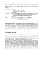
2. Verification and Identification of Speakers

Speaker recognition covers two main areas: speaker verification and speaker identification.
Speaker verification is concerned with the classification into two classes, genuine person and
impostor. In verification, an identity claim is made by an unknown speaker, and an
utterance of the unknown speaker is compared with the model for the speaker whose
identity is claimed. If the match is above a certain threshold, the identity claim is verified.
Figure 1 shows the basic structure of a speaker verification system. A high threshold makes
it difficult for impostors to be accepted by the system, but at the risk of rejecting the genuine
person. Conversely, a low threshold ensures that the genuine person is accepted

consistently, but at the risk of accepting impostors. In order to set a threshold at a desired
level of user acceptance and impostor rejection, it is necessary to know the distribution of
customer and impostor scores.










Fig. 1. Basic structure of speaker verification system.

Similarity
Decision
Feature
Extraction
Threshold
Speech
Input
Speaker ID
Verification
Result
(Accept / Reject)
Threshold
Threshold
Reference
Template

(Speaker # )

Automatic Speaker Recognition by Speech Signal

43
There are two corresponding types of errors, namely the rejection of genuine speakers, often
called false rejection, and the acceptance of impostors, often called false acceptance. The
most common performance measure used for comparing speaker verification systems is the
equal error rate. The equal error rate is found by adjusting the threshold value until the false
acceptance rate is equal to the false rejection rate. In most cases, this value must be
determined experimentally by collecting the recognition scores for a large number of both
accepting and rejecting comparisons. This involves applying an a-posteriory threshold. An
illustration of an error rate graph is shown in Figure 2. The use of an equal error rate implies
a perfect choice of threshold, which is not possible in a real application since the threshold
would have to be determined a-priory. This problem can be solved using probability theory.
The threshold for speaker verification must be updated with long-term voice variability
(Matsui et al., 1996).


Threshold
Error Rate
False Rejection
False Acceptance
0
Equal
Error Rate


Fig. 2. False rejection rate and false acceptance rate as a function of the decision threshold.

In speaker identification, a speech utterance from an unknown speaker is analysed and
compared with models of known speakers. The unknown speaker is identified as the
speaker whose model best matches the input utterance. Figure 3 shows the basic structure of
a speaker identification system.


Maximum
Selection
Feature
Extraction
Speech
Input
Identification
Result
(Speaker ID)
Similarity
Reference
Template or Model
(Speaker # 1)
Similarity
Reference
Template or M odel
(Speaker # N)

Fig. 3. Basic structure of speaker identification system.

There is also the case called “open set“ identification, in which a model for the unknown
speaker may not exist. In this case, an additional decision alternative, “the speaker does not
Frontiers in Robotics, Automation and Control

44
match any of the models“, is required. The fundamental difference between identification
and verification is the number of decision alternatives. In identification, the number of
decision alternatives is equal to the size of the population, whereas in verification there are
only two decision alternatives (accept or reject).

3. Text-Dependent Speaker Recognition

Speaker recognition methods can also be divided into text-dependent and text-independent
methods. The former require the speaker to provide utterances of the key words or
sentences having the same text for both training and recognition trials, whereas the latter do
not rely on a specific text being spoken. The text-dependent methods are usually based on
template matching techniques in which the time axes of an input speech sample and each
reference template or reference model of registered speakers are aligned, and the similarity
between them accumulated from the beginning to the end of the utterance is calculated. The
structure of text-dependent recognition systems is, therefore, rather simple. Since this
method can directly exploit the voice individuality associated with each phoneme or
syllable, it generally achieves higher recognition performance than the text-independent
method.

3.1 Effectiveness of Various Phonemes for Speaker Recognition
The speaker-specific information contained in short-term spectra was used in the initial
experiments. Twelve male speakers read the same text twice. The signal was sampled at 22
kHz with 16-bit linear coding. The speech signals were labeled using own tool (Sigmund &
Jelinek, 2005), and a log-power spectrum (128 point FFT) was calculated in the centre of
continuant sounds. The spectral channel containing maximum intensity was then set at 0 dB.
The reference samples were created by averaging three spectra. Finally, the spectra were
compared by a distance measure derived from a correlation based similarity measure

yx

yx >
<
−=
,
1d
(1)

where x and y represent the spectral vectors. Each phoneme in the test was compared with
each of the corresponding reference phonemes. The reference sample with the minimal
distance was considered to be identified. The identification rate varies from 11% to 72%. The
results obtained indicate that an individual analysis of each phoneme is impossible but that
the data can be reasonably grouped into phonetically defined classes. Table 1 gives average
identification rates. Thus, in terms of speaker-recognition power, the following ranking of
phoneme classes results:
vowels, nasals > liquids > fricatives, plosives.
As expected, vowels and nasals are the best phonemes for speaker identification. They are
relatively easy to identify in speech signal and their spectra contain features that reliably
distinguish speakers. Nasals are of particular interest because the nasal cavities of different
speakers are distinctive and are not easily modified (except when nasal congestion). For our
purposes, Table 1 gives a preliminary general overview of the results.
Automatic Speaker Recognition by Speech Signal

45

Table 1. Speaker identification rate by phoneme classes.

Two experiments were then performed on the data set within the vowel class. Because of the
formant (i.e. local maxima) structure of vowel spectra the identification rate for each vowel
can be estimated. In Table 2, individual vowels are compared in terms of speaker-
recognition power.

Table 2. Speaker identification rate by individual vowels.

It is known that different speakers show not only different formant values but exhibit
different arrangements in their vowel systems. The general distribution patterns of vowels
in formant planes can be used to build up a feature matrix for the vowel system of
individual speakers. Table 3 shows the identification rate for various numbers of different
vowels. The test started with only one vowel (the most effective) and successively other
vowels were added one by one according to their individual effectiveness as ranked in Table
2. The identification rate increased almost logarithmically from 76.2% using the one
individually best vowel “e“ up to 97.4% using all the five vowels simultaneously.

No. of Vowels Vowels Identification Rate (in %)
1 e 76.2
2 e, a 88.7
3 e, a, u 93.8
4 e, a, u, o 95.6
5 e, a, u, o, i 97.4
Table 3. Speaker identification rate depending on number of vowels used.
Phoneme Class Identification Rate (in %)
Vowels (a, e, i, o, u) 68
Nasals (m, n) 67
Liquids (l, r) 53
Fricatives (f, s, sh, z) 46

Plosives (p, t, b, d, g) 32
Vowel No. of Vowels in Test Identification Rate (in %)
i 117 52.7
o 106 61.4
u 85 68.2
a 121 74.8
e 122 76.2
Frontiers in Robotics, Automation and Control

46
3.2 Effectiveness of Speech Features in Speaker Recognition
In order to see which features are effective for speaker recognition, we studied here the
following six parametric representations: 1) autocorrelation coefficients; 2) linear prediction
(LP) coefficients; 3) log area ratios; 4) cepstral coefficients; 5) mel-cepstral coefficients; 6) line
spectral-pair (LSP) frequencies. More details how to compute these parameters could be
found in (Rabiner & Juang, 1993). Although all of these representations provide equivalent
information about the LP power spectrum, it is only the LSP representation that has the
localized spectral sensitivity property. As can be seen in Section 3.1, the vowel phonemes
result the best in recognition performance regarding the speaker identification rate. Thus,
the vowels as speech data used for this purpose were derived from utterances spoken by
nine male speakers. These utterances were low-pass filtered at 4 kHz and sampled at 10
kHz. The steady-state part of the vowel segment was located manually.
For each speaker and for each feature set the first ten coefficients were used. The Euclidean
distance was obtained by comparing a test vector against a template. A match was detected
based on the minimum distance criterion, if the intra-speaker distance was shorter than all
the inter-speaker distances. Otherwise a mismatch was declared. These matches and
mismatches were registered in the confusion matrices for each parametric representation.
Table 4 shows recognition rates for all six parametric representations mentioned above.
From these results, it can be seen that for text-dependent speaker recognition the
autocorrelation coefficients are not very effective, the log area ratio coefficients set generally

surpasses any other feature sets, and mel-cepstral coefficients are comparable with LSP
frequencies in recognition performance. In order to compute the text-dependent speaker
recognition performance for each feature set, the following procedure was used. For each
vowel, five repeats were used as the training set and about thirty randomly chosen vowels
were used as the test set; all this for a given speaker. The training set and the test set were
disjunct.

Parameters Test Patterns Recognition Rate (in %)
Autocor. coeffs. 270 61.3
LP coeffs. 268 83.7
Log area ratios 254 94.1
Cepstral coeffs. 262 87.5
Mel-Cepstal coeffs. 249 91.2
LSP frequencies 241 90.8

Table 4. Performance of vowel-dependent speaker recognizer using various parametric
representations.

4. Text-Independent Speaker Recognition

There are several applications in which predetermined key words cannot be used. In
addition, human beings can recognize speakers irrespective of the content of the utterance.
Therefore, text-independent methods have recently been actively investigated. Another
advantage of text-independent recognition is that it can be done sequentially, until a desired
Automatic Speaker Recognition by Speech Signal

47
significance level is reached, without the annoyance of repeating the key words again and
again. In text-independent speaker recognition, the words or sentences used in recognition
trials cannot generally be predicted. For this recognition, it is important to remove

silence/noise frames from both the training and testing signal to avoid modeling and
detecting the environment rather than the speaker.

4.1 Long-Term Based Methods
As text-independent features, long-term sample statistics of various spectral features, such
as the mean and variance of spectral features over a series of utterances, are used (see Fig. 4).
However, long-term spectral averages are extreme condensations of the spectral
characteristics of a speaker’s utterances and, as such, lack the discriminating power included
in the sequences of short-term spectral features used as models in text-dependent methods.
The accuracy of the long-term averaging methods is highly dependent on the duration of
the training and test utterances, which must be sufficiently long and varied.

Store
Comparison
with Threshold
Speech
Input
Decision
Voiced/
Unvoiced
Features
Extraction
Calculation:
* Means
* Variances
* Histo
g
rams
* Correlation
of Features

Speaker
Identification


Fig. 4. Typical structure of the long-term averaging system.

4.2 Average Vocal Tract Spectrum
In a long-time average spectrum of a speech signal the linguistic information (coded as
frequency variation with time) is lost while the speaker specific information is retained. In
this study, a speaker analysis approach based on linear predictive coding (LPC) is
presented. The basic idea of the approach is to evaluate an average long-time spectrum
corresponding to the anatomy of the speaker’s vocal tract independent of the actually
pronounced phoneme. First, we compute the short-time autocorrelation coefficients R
j
(k),
k=1, ,K for the j-th frame (20 msec) of speech signal s (n)

() ()( )
R k sn sn kj
n
Nk
=+
=
−
∑
1
(2)

where N is the number of samples in each frame, and then we compute the K average
autocorrelation coefficients

() ()
Rk
J
Rk
j
j
J
=
=
∑
1
1
(3)