Frontiers in Robotics, Automation and Control Part 11 pptx

15

Robust Position Estimation of an Autonomous
Mobile Robot

Touati Youcef, Amirat Yacine*, Djamaa Zaheer* & Ali-Chérif Arab
University Paris 8 Saint-Denis
France
*University Paris 12 Val de Marne
France

1. Introduction

In the past few years, the topic of localization has received considerable attention in the
research community and especially in mobile robotics area (Borenstein, 1996). It consists of
estimating the robot’s pose (position, orientation) with respect to its environment from
sensor data. Therefore, better sensory data exploitation is required to increase robot’s
autonomy. The simplest way to estimate the pose parameters is integration of odometric
data which, however, is associated with unbounded errors, resulting from uneven floors,
wheel slippage, limited resolution of encoders, etc. However, such a technique is not reliable
due to cumulative errors occurring over the long run. Therefore, a mobile robot must also be
able to localize or estimate its parameters with respect to the internal world model by using
the information obtained with its external sensors. In system localization, the use of sensory
data from a range of disparate multiple sensors, is to automatically extract the maximum
amount of information possible about the sensed environment under all operating
conditions.
Usually, for many problems like obstacle detection, localization or Simultaneous
Localization and Map Building (SLAM) (Montemerlo et al., 2002), the perception system of a
mobile robot relies on the fusion of several kinds of sensors like video cameras, radars,
dead-reckoning sensors, etc. The multi-sensor fusion problem is popularly described by
state space equations defining the interesting state, the evolution and observation models.

Based on this state space description, the state estimation problem can be formulated as a
state tracking problem. To deal with this state observation problem, when uncertainty
occurs, the probabilistic Bayesian approaches are the most used in robotics, even if new
approaches like the set-membership one (Gning & Bonnifait, 2005) or Belief theory (Ristic
and Smets, 2004) have proved themselves in some applications.
SLAM is technique used by mobile robots to build up a map within an unknown
environment while at the same time keeping track of their current position. Several works
implementing SLAM algorithms have been studied extensively over the last years in this
direction, leading to approaches that can be classified into three well differentiated
paradigms depending on the underlying map structure: metric (Sim et al., 2006) (Tardos et
Frontiers in Robotics, Automation and Control

294
al., 2002), topological (Ranganathan et al., 2006) (Savelli & Kuipers, 2004), or hybrid
representations (Estrada et al., 2005) (Kuipers & Byun, 2001) (Dissanayake et al., 2001)
(Thrun et al., 2004). These techniques deal mainly with the localization problem using
mainly visual features and exteroceptive sensors, such as camera, GPS unit or laser scanner.
Localization algorithms have also been developed in sensors networks and applied in a
myriad of applications such as intrusion detection, road traffic monitoring, health
monitoring, reconnaissance and surveillance. Their main objectives is to estimate the
location of sensors with initially unknown location information by using knowledge for
absolute positions of a few sensors and their inter-sensor measurements such as distance
and bearing measurements (Chong & Kumar, 2003) (Mao et al., 2007).
Ubiquitous computing technology is gradually being used to analyze people’s activities. In
this case, several research efforts on localization function have been conducted into
recognizing human position and trajectories (Letchner et al., 2005) (Madhavapeddy & Tse,
2005) (Kanda et al., 2007). For example, Liao et al. used locations obtained via GPS with
relational Markov model to discriminate location-based activities (Liao et al., 2005). Wen et
al. developed an approach for inhabitant location and tracking system in a cluttered home
environment via floor load sensors (Liau et al., 2008). In this approach, a probabilistic data

association technique is applied to analyze the cluttered pressure readings collected by the
load sensors so as to track their movements.
The main idea of data fusion methods is to provide a reliable estimation of robot’s pose,
taking into account the advantages of the different sensors (Harris, 1998). The main data
fusion applied methods are very often based on probabilistic methods, and indeed
probabilistic methods are now considered the standard approach to data fusion in all
robotics applications. Probabilistic data fusion methods are generally based on Bayes’ rule
for combining prior and observation information. Practically, this may be implemented in a
number of ways: through the use of the Kalman and extended Kalman filters, through
sequential Monte Carlo methods, or through the use of functional density estimates.
There are a number of alternatives to probabilistic methods. These include the theory of
evidence and interval methods. Such alternative techniques are not as widely used as they
once were, however they have some special features that can be advantageous in specific
problems.
The rest of the presented work is organized as follows. Section 2 discusses the problem
statement and related works in the field of multi-sensor data fusion for the localization of a
mobile robot. Section 3 describes the global localization system which is considered. We
develop the proposed robust pose estimation algorithm in section 4 and its application is
demonstrated in section 5. Simulation results and a comparative analysis with standard
existing approaches are also presented in this section.

2. Background & related works

The Kalman Filter (KF) is the best known and most widely applied parameter and state
estimation algorithm in data fusion methods (Gao, 2002). Such a technique can be
implemented from the kinematic model of the robot and the observation (or measurement)
model, associated to external sensors (gyroscope, camera, telemeter, etc.). The Kalman filter
has a number of features which make it ideally suited to dealing with complex multi-sensor
estimation and data fusion problems. In particular, the explicit description of process and
Robust Position Estimation of an Autonomous Mobile Robot

295
observations allows a wide variety of different sensor models to be incorporated within the
basic algorithm. In addition, the consistent use of statistical measures of uncertainty makes
it possible to quantitatively evaluate the role each sensor plays in overall system
performance. Further, the linear recursive nature of the algorithm ensures that its
application is simple and efficient. For these reasons, the Kalman filter has found wide-
spread application in many different data fusion problems (Bar-Shalom, 1990) (Bar-Shalom
& Fortmann, 1988) (Maybeck, 1979). In robotics, the KF is most suited to problems in
tracking, localisation and navigation; and less so to problems in mapping. This is because
the algorithm works best with well defined state descriptions (positions, velocities, for
example), and for states where observation and time-propagation models are also well
understood.
The Kalman Filtering process can be considered as a prediction-update formulation. The
algorithm uses a predefined linear model of the system to predict the state at the next time
step. The prediction and updates are combined using the Kalman gain which is computed to
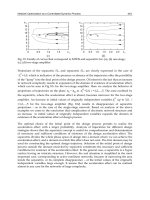
minimize the Mean Square Error (MSE) of the state estimate. Figure 1 illustrates the block
diagram of KF cycle (Bar-Shalom & Fortmann, 1988), and for further details, refer to
(Siciliano & Khatib, 2008).


Fig. 1. Block diagram of the Kalman filter cycle (Bar-Shalom & Fortmann, 1988; Siciliano &
Khatib, 2008)

The Extended Kalman Filter (EKF) is a version of the Kalman filter that can handle non-
linear dynamics or non-linear measurement equations. Like the KF, it is assumed that the
noises are all Gaussian, temporally uncorrelated and zero-mean with known variance. The
EKF aims to minimise mean-squared error and therefore compute an approximation to the
conditional mean. It is assumed therefore that an estimate of the state at time k−1 is available
which is approximately equal to the conditional mean. The main stages in the derivation of

Frontiers in Robotics, Automation and Control

296
the EKF follow directly from those of the linear Kalman filter with the additional step that
the process and observation models are linearised as a Taylor series about the estimate and
prediction, respectively. The algorithm iterates in two update stages, measurement and
time, see figure 2. Each positioning operation is generated once a new observation is
assumed. Localization can be done from odometry or visual input changes. The complete
algorithm is implemented for each landmark perception. In this sense, the processing time is
saved by reducing covariance matrix function size per landmark. Detailed computations
may be found in any number of books on the subject (Samperio & Hu, 2006).


Fig. 2. Flowchart of Extended Kalman filter Algorithm (after Samperio & Hu, 2006)

Various approaches based on EKF have been developed. These approaches work well as
long as the used information can be described by simple statistics well enough. The lack of
relevant information is compensated by using models of various processes. However, such
model-based approaches require assumptions about parameters which might be very
difficult to determine (white Gaussian noise and initial uncertainty over Gaussian
distribution). Assumptions that guarantee optimum convergence are often violated and,
therefore, the process is not optimal or it can even converge. In fact, many approaches are
based on fixed values of the measurement and state noise covariance matrices. However,
such an information is not a priori available, especially if the trajectory of the robot is not
elementary and if changes occur in the environment. Moreover, it has been demonstrated in
the literature that how poor knowledge of noise statistics (noise covariance on state and
measurement vectors) may seriously degrade the Kalman filter performance (Jetto, 1999). In
the same manner, the filter initialization, the signal-to-noise ratio, the state and observation
processes constitute critical parameters, which may affect the filtering quality. The stochastic
Kalman filtering techniques were widely used in localization (Gao, 2002) (Chui, 1987)

(Arras, 2001)(Borthwick, 1993) (Jensfelt, 2001) (Neira, 1999) (Perez, 1999) (Borges, 2003). Such
approaches rely on approximative filtering, which requires ad doc tuning of stochastic
Robust Position Estimation of an Autonomous Mobile Robot

297
modelling parameters, such as covariance matrices, in order to deal with the model
approximation errors and bias on the predicted pose. In order to compensate such error
sources, local iterations (Kleeman, 1992), adaptive models (Jetto, 1999) and covariance
intersection filtering (Julier, 1997) (Xu, 2001) have been proposed. An interesting approach
solution was proposed in (Jetto, 1999), where observation of the pose corrections is used for
updating of the covariance matrices. However, this approach seems to be vulnerable to
significant geometric inconsistencies of the world models, since inconsistent information can
influence the estimated covariance matrices.
In the literature, the localization problem is often formulated by using a single model, from
both state and observation processes point of view. Such an approach, introduces inevitably
modelling errors which degrade filtering performances, particularly, when signal-to-noise
ratio is low and noise variances have been estimated poorly. Moreover, to optimize the
observation process, it is important to characterize each external sensor not only from
statistic parameters estimation perspective but also from robustness of observation process
perspective. It is then interesting to introduce an adequate model for each observation area
in order to reject unreliable readings. In the same manner, a wrong observation leads to a
wrong estimation of the state vector and consequently degrades the performance of
localization algorithm. Multiple-Model estimation has received a great deal of attention in
recent years due to its distinctive power and great recent success in handling problems with
both structural and parametric uncertainties and/or changes, and in decomposing a
complex problem into simpler sub-problems, ranging from target tracking to process control
(Blom, 1988) (Li, 2000) (Li, 1993) (Mazor, 1996).
This paper focuses on robust pose estimation for mobile robot localization. The main idea of
the approach proposed here is to consider the localization process as a hybrid process which
evolves according to a model among a set of models with jumps between these models

according to a Markov chain (Djamaa & Amirat, 1999) (Djamaa, 2001). A close approach for
multiple model filtering is proposed in (Oussalah, 2001). In our approach, models refer here
to both state and observation processes. The data fusion algorithm which is proposed is
inspired by the approach proposed in (Dufour, 1994). We generalized the latter for multi
mode processes by introducing multi mode observations. We also introduced iterative and
adaptive EKFs for estimating noise statistics. Compared to a single model-based approach,
such an approach allows the reduction of modelling errors and variables, an optimal
management of sensors and a better control of observations in adequacy with the
probabilistic hypotheses associated to these observations. For this purpose and in order to
improve the robustness of the localization process, an on line adaptive estimation approach
of noise statistics (state and observation) proposed in (Jetto, 1999), is applied for each mode.
The data fusion is performed by using Adaptive Linear Kalman Filters for linear processes
and Adaptive EKF for nonlinear processes.

3. Localization system description

This paper deals with the problem of multi sensor filtering and data fusion for the robust
localization of a mobile robot. In our present study, we consider an autonomous robot
equipped with two telemeters placed perpendicularly, for absolute position measurements
of the robot with respect to its environment, a gyroscope for measuring robot’s orientation,
two drive wheels and two separate encoder wheels attached with optical shaft encoders for
Frontiers in Robotics, Automation and Control

298
odometry measurements. The environment where the mobile robot moves is a rectangular
room without obstacles, see figure 3.

Fig. 3. Mobile robot description and its evolution in the environment with Nominal
trajectory

The aim is not to develop a new method for environment reconstruction or modelling from
data sensors; rather, the goal is to propose a new approach to improve existing data fusion
and filtering techniques for robust localization of a mobile robot.
For an environment with a more complex shape, the observation model which has to be
employed at a given time, will depend on the robot’s situation (robot’s trajectory, robot’s
pose with respect to its environment) and on the geometric or symbolic model of
environment.
Initially, all significant information for localization is contained in a state space vector. The
usefulness of an observer in a localization system evokes the modelling of variables that
affect the entire behaviour system. The observer design problem relies on the estimation of
all possible internal states in a linear system.

3.1 Odometric model
Let
()
[]
T
e
kkykxkX )()()(
θ
= be the state vector at time k , describing the robot’s pose with
respect to the fixed coordinate system.

The kinematic model of the robot is described by the following equations:

(
)

2cos
1 kkkkk
lxx
θθ
Δ+⋅+=
+

(1)
Robust Position Estimation of an Autonomous Mobile Robot

299
(
)
2sin
1 kkkkk
lyy
θθ
Δ++=
+

(2)
kkk
θθθ
Δ+=
+1

(3)

with: 2/)(
l

k
r
kk
lll += and dll
l
k
r
kk
/)( −=Δ
θ
.
r
k
l and
l
k
l are the elementary displacements
of the right and the left wheels;
d the distance between the two encoder wheels.

3.2 observation model of telemeters
As the environment is a rectangular room, the telemeters measurements correspond to the
distances from the robot location to walls (Fig. 3.).

Then, the observation model of telemeters is described as follows:
for
()
l
k
θθ

<≤0
, according to X-axis:

(
)
(
)
(
)
(
)
(
)
kkxdkd
x
θ
cos−=

(4)

for
()
ml
k
θθθ
≤≤ , according to Y-axis:

(
)
(

)
(
)
(
)
kkydkd
y
θ
sin)( −=

(5)

With
x
d and
y
d , respectively the length and the width of the experimental site;
l
θ
and
m
θ
, respectively the angular bounds of observation domain with respect to X and Y axes;
()
kd is the distance between the robot and the observed wall with respect to X or Y axes at
time
k .

3.3 observation model of gyroscope
By integrating the rotational velocity, the gyroscope model can be expressed by the

following equation:

(
)
(
)
kk
l
θθ
=

(6)

Each sensor described above is subject to random noise. For instance, the encoders introduce
incremental errors (slippage), which particularly affect the estimation of the orientation. For
a telemeter, let’s note various sources of errors: geometric shape and surface roughness of
the target, beam width. For a gyroscope, the sources of errors are: the bias drift, the
nonlinearity in the scale factor and the gyro’s susceptibility to changes in ambient
temperature.
Frontiers in Robotics, Automation and Control

300
So, both odometric and observation models must integrate additional terms representing
these noises. Models inaccuracies induce also noises which must be taken into account. It is
well known that odometric model is subject to inaccuracies caused by factors such as:
measured wheel diameters, unequal wheel-diameters, trajectory approximation of robot
between two consecutive samples. These noises are usually assumed to be Zero-mean white
Gaussian with known covariance. This hypothesis is discussed and reconsidered in the
proposed approach.
Besides, an estimation error of orientation introduces an ambiguity in the telemeters

measurements (one telemeter is assumed to measure along X axis while it is measuring
along Y axis and vice-versa). This situation is particularly true when the orientation is near
angular bounds
l
θ
and
m
θ
. This justifies the use of multiple models to reduce measuring
errors and efficiently manage robot’s sensors. For this purpose, we have introduced the
concept of observation domain (boundary angles) as defined in equations (4) and (5).

4. Proposed approach for mobile robot localisation

As mentioned in (Touati et al., 2007), we present our data fusion and filtering approach for
the localization of a mobile robot. In order to increase the robustness of the localization and
as discussed in section 2, the localization process is decomposed into multiple models. Each
model is associated with a mode and an interval of validity corresponding to the
observation domain; the aim is to consider only reliable information by filtering erroneous
information. The localization is then considered as a hybrid process. A Markov chain is
employed for the prediction of each model according to the robot mode. The multiple
model approach is best understandable in terms of stochastic hybrid systems. The state of a
hybrid system consists of two parts: a continuously varying base-state component and a
modal state component, also known as system mode, which may only jump among points,
rather than vary continuously, in a (usually discrete) set. The base state components are the
usual state variables in a conventional system. The system mode is a mathematical
description of a certain behavior pattern or structure of the system. In our study, the mode
corresponds to robot’s orientation. In fact, the latter parameter governs the observation
model of telemeters along with observation domain. Other parameters, like velocity or
acceleration, could also be taken into account for mode’s definition. Updating of mode’s

probability is carried out either from a given criterion or from given laws (probability or
process). In this study, we assume that each Markovian jump (mode) is observable (Djamaa
2001) (Dufour, 1994). The mode is observable and measurable from the gyroscope.

4.1 Proposed filtering models
Let us consider a stochastic hybrid system. For a linear process, the state and observation
processes are given by:

()
(
)
(
)
()( )()
kkk
kekke
kWkUkB
kkXAkkX
ααα
ααα
,,1,
,1/1,1/
+−⋅+
−−⋅=−

(7)
()
(
)
(

)
(
)
kkekke
kVkkXCkY
αααα
,,1/, +−⋅=

(8)

Robust Position Estimation of an Autonomous Mobile Robot

301
For a nonlinear process, the state and observation processes are described by:

(
)
(
)
(
)
(
)
()
k
keke
kW
kUkkXFkkX
α
αα

,
1,,1/1,1/
+
−−−=−

(9)
(
)
(
)
(
)
(
)
kkeeke
kVkkXGkY
ααα
,,1/, +−=

(10)

where
e
X ,
e
Y and U are the base state vector, noisy observation vector and input vector;
k
α
is the modal state or system mode at time k, which denotes the mode during the k
th

sampling period;
W and V are the mode-dependent state and measurement noise
sequences, respectively.

The system mode sequence
k
α
is assumed for simplicity to be a first-order homogeneous
Markov chain with the transition probabilities, so for S
ji
∈∀
αα
, :

{
}
ij
i
k
j
k
P
παα
=
+
|
1

(11)

Where
j
k
α
denotes that mode
j
α
is in effect at time k and S is the set of all possible system
modes, called mode space.

The state and measurement noises are of Gaussian white type. In our approach, the state
and measurement processes are assumed to be governed by the same Markov chain.
However, it’s possible to define differently a Markov chain for each process. The Markov
chain transition matrix is stationary and well defined.

4.2 Statistics parameters estimation
It is well known that how poor estimates of noise statistics may lead to the divergence of
Kalman filter and degrade its performance. To prevent this divergence, we propose an
adaptive algorithm for the adjustment of the state and measurement noise covariance
matrices.

a. Measurement noise variance
Let
()
(
)
kR
i
2

,
ν
σ
=
()
0
:1 ni = , be the measurement noise variance at time k for each
component of the observation vector. Parameter
0
n denotes the number of observers
(sensors number).

Let
()
k
β
ˆ
the squared mean error for stable measurement noise variance, and
()
k
γ
the
innovation, thus:

Frontiers in Robotics, Automation and Control

302
() ()
∑
=

−=
n
j
i
k
n
k
0
2
1
1
ˆ
γβ

(12)

For 1+n samples, the variance of
(
)
k
β
ˆ
can be written as:

()
()
(
)
(
)

()
∑
=
⎟
⎟
⎠
⎞
⎜
⎜
⎝
⎛
+−
⋅−−−⋅−
+
=
n
j
i
T
i
i
jkC
jkjkPjkC
n
kE
0
2
,
1,
1

1
ˆ
ν
σ
β

(13)

Then, we obtain the estimation of the measurement noise variance:

() ()
()()
⎪
⎭
⎪
⎬
⎫
⎪
⎩
⎪
⎨
⎧
⎟
⎟
⎟
⎠
⎞
⎜
⎜
⎜

⎝
⎛
−⋅−−−
⋅−⋅
+
−−
=
∑
=
n
j
T
i
ii
i
jkCjkjkP
jkC
n
n
jk
n
0
2
2
,
0,
1,
1
1
max

ˆ
γ
σ
ν

(14)

The restriction with respect to zero is related to the notion of variance. A recursive
formulation of the previous estimation can be written:

() ( )
()
()()
⎪
⎪
⎪
⎭
⎪
⎪
⎪
⎬
⎫
⎪
⎪
⎪
⎩
⎪
⎪
⎪
⎨

⎧
⎟
⎟
⎟
⎟
⎟
⎟
⎠
⎞
⎜
⎜
⎜
⎜
⎜
⎜
⎝
⎛
Ψ⋅
+
−
+−−⋅+−= 0,
1
1
1
1
ˆ
max
ˆ
2
2

2
,
2
,
n
n
nk
k
n
kk
i
i
ii
γ
γ
σσ
νν

(15)

where:

(
)
(
)
(
)
(
)

(
)
()()()()()
T
i
i
T
ii
nkCnknkP
nkCkCkkPkC
111,1
11,
+−⋅−+−+−
⋅+−−⋅−⋅=Ψ

(16)

b. State noise variance
To estimate the state noise variance, we employ the same principle as in subsection a. One
can write:

(
)
(
)
dine
QkkQ ⋅=
2
,
ˆ

ˆ
σ

(17)

By assuming that noises on the two encoder wheels measurements obey to the same law
and have the same variance, the estimation of state noise variance can be written:

Robust Position Estimation of an Autonomous Mobile Robot

303
()
(
)
(
)
(
)
() ()
() ()
⎪
⎪
⎭
⎪
⎪
⎬
⎫
⎪
⎪
⎩

⎪
⎪
⎨
⎧
+⋅⋅+
+−+
⋅+⋅+−−
=
0
,
11
1
ˆ
1
,111
max
ˆ
2
,
2
2
,
T
idi
i
T
i
ii
in
kCQkC

kkC
kkPkCk
k
ν
σ
γ
σ

(18)

with:

(
)
(
)
(
)
T
d
kBkBkQ ⋅=
ˆ

(19)

By replacing the measurement noise variance by its estimate, we obtain a mean value given
by the following equation:

()
()

()
⎪
⎭
⎪
⎬
⎫
⎪
⎩
⎪
⎨
⎧
−
⋅+
=
∑∑
==
0,
ˆ
1
1
max
ˆ
11
2
,
0
2
0
m
j

n
i
inn
jk
nm
k
σσ

(20)

Where, the parameter m represents the sample number.

The algorithm proposed above carries out an on line estimation of state and measurement
noise variances. Parameters n and m are chosen according to the number of samples used
at time
k . The noises variances are initialized from an “a priori” information and then
updated on line. In our approach, variances are updated according the robot’s mode and the
measurement models.
For an efficient estimation of noise variances, an ad hoc technique consisting in a measure
selection is employed. This technique consists of filtering unreliable readings by excluding
readings with weak probability like the appearance of fast fluctuations. For instance, in the
case of Gaussian distribution, we know that about 95% of the data are concentrated in the
interval of confidence
[
]
σσ
2,2 +− mm where m represents the mean value and
σ
the
variance.

The sequence in which the filtering of the state vector components is carried out is
important. Once the step of filtering completed, the probabilities of each mode are updated
from the observers (sensors). One can note that the proposed approach is close, on one
hand, to the Bayesian filter by the extrapolation of the state probabilities, and on the other
hand to the filter with specific observation of the mode.

5. Implementation and results

The proposed approach for robust localization was applied for the mobile robot described in
section 2. The nominal trajectory of the mobile robot includes three sub trajectories T1, T2
and T3, defining respectively a displacement along X axis, a curve and a displacement along
Y axis, see figure 4.
Frontiers in Robotics, Automation and Control

304
X
Y
T
1
T
2

T
3

θ

l

θ

m





Fig. 4. Mobile robot in moving in the environment with Nominal trajectory T1, T2 and T3.

Note that the proposed approach remains valid for any type of trajectory (any trajectory can
be approximated by a set of linear and circular sub trajectories). For our study, we have
considered three models. This number can be modified according to the environment’s
structure, the type of trajectory (robot rotating around itself, forward or backward
displacement, etc.) and to the number of observers (sensors). Notice that the number of
models (observation and state) has no impact on the validity of the proposed approach.
To demonstrate the validity of our proposed Adaptive Multiple-Model approach and to
show its effectiveness, we’ve compared it to the following standard approaches: Single-
Model based EKF without estimation variance, single-model based IEKF. For sub
trajectories T1 and T3, filtering and data fusion are carried out by iterative linear Kalman
filters due to linearity of the models, and for sub trajectory T2, by iterative and extended
Kalman filters.
The observation selection technique is applied for each observer before the filtering step in
order to control, on one side, the estimation errors of variances, and on the other side, after
each iteration, to update the state noise variance. If an unreliable reading is rejected at a
given filtering iteration, this has for origin either a bad estimation of the next component of
the state vector and of the prediction of the corresponding observation, or a bad updating of
the corresponding state noise variance. The iterative filtering is optimal when it is carried
out for each observer and no reading is rejected. In the implementation of the proposed
approach, the state noise variance is updated, for a given mode
i

, is carried out according to
the following filtering sequence: x, y and then
θ
.
Robust Position Estimation of an Autonomous Mobile Robot

305
Firstly, let’s consider the set of the following notations, table 1:

(
x
ε
, y
ε
,
εθ
) Estimation errors corresponding to (
x
, y ,
θ
)
( Ndx , Ndy ,
θ
Nd )
Percentage of selected data for filtering corresponding to
(
x
, y ,
θ
)

( Ndxe , Ndye , eNd
θ
)
Percentage of selected data for estimation of the variances of
state and measurement noises, corresponding to (
x
, y ,
θ
)
SM ( -+ ) Single-Model based EKF
SMI ( ° ) single-model based IEKF
AMM ( - - ) Adaptive Multiple-Model
Table 1. Set of notations

Several scenarios have been studied according to the variation of statistics parameters, i.e.,
sensors signal-to-noise ratio, initial state variance, noise statistics (measurement and state
variances). Simulations were carried out to analyze the performances of each approach in
various scenarios. Thus, in scenarios 1 and 2, we show the influence of measurement and
state noises variances estimation on the quality of localization. In scenario 3, it will concern
the sensors signal-to-noise ratio.

Scenario 1
:
-Noise-to-signal Ratio of odometric sensors: right encoder: 4%, left encoder: 4%
-Noise-to-signal Ratio of Gyroscope: 1%
-Noise-to-signal Ratio of telemeters: 2% of the odometric elementary step
-“A priori” knowledge on the variance in initial state: Good
-“A priori” knowledge on measurement noise variances: Good
-State and measurement noise variances estimation: 10 times real average variances of
encoders

This scenario is characterized by weak state and measurement noises and by high initial
value of state noise variance. One can note that although a bad initialization (10 times the
average variance), the AMM approach presents better performances for estimation of the 3
components of state vector (Tables 2-4, figures 5-11). On section T1, (figure 12), the
estimated variance remains constant compared to the a priori average variance (10 times the
average variance) corresponding to the initial state. Indeed, the algorithm of estimation of
variances does not show any evolution because of the high value of variance in the initial
state. However, for section T2 and T3, the variance decreases by half compared to the initial
variance, and approaches the actual average variance.

Frontiers in Robotics, Automation and Control

306

T1 T2 T3

SM SMI AMM

SM SMI AMM

SM SMI AMM
x
ε
(cm) 3.46 6.12 0.64 8.3 6.15 9.6 4.76 3.38 0.72
y
ε
(cm) 4.58 3.69 0.5 12.3 7.3 9.7 4.64 3.58 1.82
εθ
(10

-3
rad)
22.7 30.5 2.7 8.2 11.9 9.7 21.6 29.3 7.9
Table 2. Average estimation errors

Ndx
Ndy
θ
Nd
Ndxe

Ndye

eNd
θ

98.75% 90% 97.5% 98.75% 98.75% 97.5%
Table 3. Selected data percentage


Fig. 5. Estimated trajectories by Encoders and, SM, SMI and AMM Filters


Fig. 6. Estimated trajectories (sub trajectory T1)
Robust Position Estimation of an Autonomous Mobile Robot

307

Fig. 7. Estimated trajectories (sub trajectory T2)

Fig. 8. Estimated trajectories (sub trajectory T3)


Samples
Fig. 9. Position error with respect to X axis
Frontiers in Robotics, Automation and Control

308

Samples
Fig. 10. Position error with respect to Y axis


Samples
Fig. 11. Absolute error on orientation angle


Samples
Fig. 12. Ratio between the estimate of state noise variance and the average variance
Robust Position Estimation of an Autonomous Mobile Robot

309
Scenario 2:
-Noise-to-signal Ratio of odometric sensors: right encoder: 10%, left encoder: 10%
-Noise-to-signal Ratio of Gyroscope: 3%
-Noise-to-signal Ratio of telemeters: 4% of the odometric elementary step (40% of the state
noise)
-“A priori” knowledge on the variance in initial state: Good
-“A priori” knowledge on noise variances (i) telemeters and state: Good; (ii) gyroscope: Bad

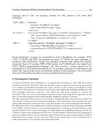
The results presented here (Tables 4-5 and figures 13-20) show the influence of signal-to-
noise ratio and estimation of noise variances on performances of SM and SMI filters. In this
scenario, the initial variance of measurement noise of the gyroscope is incorrectly estimated.
Unlike AMM approach, filters SM and SMI do not carry out any adaptation of this variance,
leading to unsatisfactory performance.


T1 T2 T3

SM SMI AMM

SM SMI AMM

SM SMI AMM
x
ε
(cm) 11.7 11 1.8 19 75 13.6 17.3 40 1.3
y
ε
(cm) 16.7 21 1 39 179 17.4 15.7 117 1.93
εθ
(10
-3
rad)
99.3 129 1.5 42.9 175 35.4 97.5 167 37.8
Table 4. Average estimation errors

Ndx
Ndy

θ
Nd
Ndxe

Ndye

eNd
θ

87.5% 66% 99.37% 87.5% 82.5% 99.37%
Table 5. Selected data percentage

Figure 20 illustrates the evolution of state noise variance estimate compared to the average
variance. Note that the ratio between variances reaches 1.7 on sub trajectory T1, 3.0 on sub
trajectory T2, and 3.3 on sub trajectory T3. It is important to mention that the algorithm
proposed for estimation of variances estimates the actual value of state noise variance and
not its average value. These results are related to the fact that the signal-to-noise ratio is
weak both for the odometer and the telemeters.


Fig. 13. Estimated trajectories by Encoders and, SM, SMI and AMM Filters
Frontiers in Robotics, Automation and Control

310

Fig. 14. Estimated trajectories (sub trajectory T1)


Fig. 15. Estimated trajectories (sub trajectory T2)

Fig. 16. Estimated trajectories (sub trajectory T3)

Robust Position Estimation of an Autonomous Mobile Robot

311

Samples
Fig. 17. Position error with respect to X axis


Samples
Fig. 18. Position error with respect to Y axis


Samples
Fig. 19. Absolute error on orientation angle
Frontiers in Robotics, Automation and Control

312

Samples
Fig. 20. Ratio between the estimate of state noise variance and the average variance

Scenario 3:
-Noise-to-signal Ratio of odometric sensors: right encoder: 8%, left encoder: 8%
-Noise-to-signal Ratio of Gyroscope: 3%
-Noise-to-signal Ratio of telemeter 1: 10% of the odometric elementary step
-Noise-to-signal Ratio of telemeter 2: 10% the odometric elementary step
-“A priori” knowledge on the variance in initial state: Good

-“A priori” knowledge on noise statistics (measurement and state variances): Good

In this scenario, the telemeters measurement noise is higher than state noise. We remark that
performances of AMM filter are better that those of SM and SMI filters concerning x and y
components (tables 6-7; figures 21-28). In sub trajectory T3, the orientation’s estimation error
relating to AMM filter (Table 6) has no influence on filtering quality of the remaining
components of state vector. Besides, one can note that this error decreases in this sub
trajectory, see figure 27. In this case, only one gyroscope is used for the prediction and
updating the Markov chain probabilities. In sub trajectory T2, we remark that the estimation
error along x-Axis for AMM filter is lightly higher than those relating to other filters. This
error is concentrated on first half of T2 sub trajectory (figure 25) and decreases then on
second half of the trajectory. This can be explained by the fact that on one hand, the
estimation variances algorithm rejected 0.7% of data, and on the other hand, the filtering
step has rejected the same percentage of data. This justifies that neither the variances
updating, nor the x-coordinate correction, were carried out (figure 28).
Note that unlike filters SM and SMI, filter AMM has a robust behavior concerning pose
estimation even when the signal-to-noise ratio is weak. By introducing the concept of
observation domain for observation models, we obtain a better modeling of observation and
a better management of robot’s sensors. The last remark is related to the bad performances
of filters SM and SMI when the signal-to-noise ratio is weak. This ratio degrades the
estimation of the orientation angle, observation matrices, Kalman filter gain along with the
prediction of the observations.

Robust Position Estimation of an Autonomous Mobile Robot

313

Fig. 21. Estimated trajectories by Encoders and, SM, SMI and AMM Filters

Fig. 22. Estimated trajectories (sub trajectory T1)


Fig. 23. Estimated trajectories (sub trajectory T2)
Frontiers in Robotics, Automation and Control

314

Fig. 24. Estimated trajectories (sub trajectory T3)


T1 T2 T3

SM SMI AMM

SM SMI AMM

SM SMI AMM
x
ε
(cm) 6.25 3.23 2.5 13.2 10.8 15.3 31.9 31.2 1.2
y
ε
(cm) 13.6 16.7 2.3 23.9 11.9 8.25 19.2 5.75 3.23
εθ
(10
-3
rad)
81.1 66.9 3.8 32.2 39.9 35.6 136 125 267.9
Table 6. Average estimation errors (Scenario 1)

Ndx
Ndy
θ
Nd
Ndxe

Ndye

eNd
θ

99.37% 84.37% 99.37% 99.37% 97.5% 99.37%
Table 7. Selected data percentage


Samples
Fig. 25. Position error with respect to X axis
Robust Position Estimation of an Autonomous Mobile Robot

315

Samples
Fig. 26. Position error with respect to Y axis


Samples
Fig. 27. Absolute error on orientation angle

Samples
Fig. 28. Ratio between the estimate of state noise variance and the average variance

6. Conclusion

This research work introduces a multiple model approach for the robust localization of a
mobile robot. The localization method is considered as a hybrid process, which is
Frontiers in Robotics, Automation and Control

316
decomposed into multiple models. Each model is associated with a mode and an interval of
validity corresponding to the observation domain. A Markov chain is employed for the
prediction of each model according to the robot mode. To prevent divergence of standard
Kalman Filtering and to increase its robustness, we proposed an adaptive algorithm for the
adjustment of the state and measurement noise covariance matrices. For an efficient
estimation of noise variances, we introduced an ad hoc technique consisting in a measure
selection for filtering unreliable readings. The simulation results we obtain in different
scenarios show better performances of the proposed approach compared to standard
existing filters. Some future research need to be conducted to complete the proposed
approach and particularly in probabilistic data fusion through sequential Monte Carlo
methods, or through the use of functional density estimates. These investigations into
utilizing multiple model technique for robust localization show promise and demand
continuing research. Fuzzy logic theory can also be considered to increase robustness of the
proposed localization algorithm.

7. References

Arras, K.O.; Tomatis, N.; Jensen, B.T.; Siegwart, R. (2001). Multisensor on-the-fly
localization: precision and reliability for applications, Robotics and Autonomous
Systems, 34, 131–143

Bar-Shalom, Y. (1990). Multi-target multi-sensor tracking (Artec House, Norwood 1990)
Bar-Shalom, Y. & Fortmann, T.E. (1988). Tracking and data association, (Academic, New
York 1988)
Blom, H. A.P. & Bar-Shalom, Y. (1998). The interacting multiple model algorithm for
systems with Markovian switching coefficients, IEEE Transactions Automation and
Control, Vol. 33, pp. 780–783
Borenstein, J.; Everett, B. & Feng, L. (1996). Navigating mobile robots: systems and
techniques, A.K. Peters, Ltd., Wellesley, MA
Borges, G.A. & Aldon, M.J. (2003). Robustified estimation algorithms for mobile robot
localization based geometrical environment maps, Robotics and Autonomous Systems,
45 (2003) 131-159
Borthwick, S.; Stevens, M. & Durrant-Whyte, H. (1993). Position estimation and tracking
using optical range data, Proceedings of the IEEE/RSJ International Conference on
Intelligent Robots and Systems, pp. 2172–2177
Chong, C.Y. & Kumar, S. (2003). Sensor networks: evolution, opportunities and challenges,
Proceeding of the IEEE, Vol.91, No. 8, pp. 1247-1256
Chui, C. & Chen, G. (1987). Kalman filtering with real time applications, Springer Series in
Information Sciences, Springer-Verlag, New-York 17 23-24
Dissanayake, G.; Newman, P.; Clark, S.; Durrant-Whyte, H. & Csorba, M. (2001). A Solution
to the simultaneous localization and map building (SLAM) problem, IEEE
Transactions on Robotics and Automation, Vol.17, No.3, pp. 229-241
Djamaa, Z. & Amirat, Y. (1999). Multi-model approach for the localization of mobile robots
by multisensor fusion, Proceedings of the 32th International Symposium On Automotive
Technology and Automation, pp. 247-260, Vienna, Austria
Djamaa, Z. (2001)., Approche multi modèle à sauts Markoviens et fusion multi capteurs
pour la localisation d’un robot mobile. PhD Thesis, Paris XII University, France
Robust Position Estimation of an Autonomous Mobile Robot

317
Dufour, F. (1994). Contribution à l’étude des systèmes linéaire à saut markoviens, PhD

Thesis, University of Paris Sud University, France
Estrada, C.; Neira, J. & Tardós, J.D. (2005). Hierarchical SLAM: real-Time accurate mapping
of large environments, IEEE Transactions on Robotics, Vol. 21, No. 4, pp. 588-596
Gao, J.B. & Harris, C.J. (2002). Some remarks on Kalman filters for the multi-sensor fusion,
Journal of Information Fusion, 3 191-201
Gning, A. & Bonnifait, P. (2005). Dynamic vehicle localization using constraints Propagation
techniques on intervals. A comparison with Kalman Filtering. Proceedings of the
International Conference on Robotics and Automation, pp. 4144- 4149, ISBN: 0-
7803-8914-X, Barcelona, Spain
Harris, C.; Bailley, A. & Dodd, T. (1998). Multi-sensor data fusion in defense and aerospace,
Journal of Royal Aerospace Society, 162 (1015) 229-244
Jensfelt, P. & Christensen, H.I.(2001). Pose tracking using laser scanning and minimalistic
environment models, IEEE Transactions on Robotics and Automation, 17 (2) 138–147
Jetto, L.; Longhi, S. & Venturini, G. (1999) Development and experimental validation of an
adaptive Kalman filter for the localization of mobile robots, IEEE Transactions on
Robotics and Automation, 15 (2) 219–229
Julier, S.J. & Uhlmann, J.K. (1997) A non-divergent estimation algorithm in the presence of
unknown correlations, Proceedings of the American Control Conference
Kanda, T.; Shiomi, M.; Perrin, L.; Nomura, T.; Ishiguro, H. & Hagita, N. (2007). Analysis of
people trajectories with ubiquitous sensors in a science museum, IEEE International
Conference on Robotics and Automation, pp.4846-4853, Roma, Italy
Kleeman, L. (1992). Optimal estimation of position and heading for mobile robots using
ultrasonic beacons and dead-reckoning, Proceedings of the IEEE International
Conference on Robotics and Automation, pp. 2582–2587
Kuipers, B. & Byun, Y.T. (2001). A robot exploration and mapping strategy based on a
semantic hierarchy of Spatial Representations, Robotics and Autonomous Systems,
Vol. 8, pp. 47-63
Li, X. R. (2000). Engineer’s guide to variable-structure multiple-model estimation for
tracking, in Multitarget-Multisensor Tracking: Applications and Advances, Y. Bar-
Shalom and D.W. Blair, Eds. Boston, MA: Artech House, Vol. 3, Chap. 10, pp. 499–

567
Li, X. R. (1996). Hybrid estimation techniques, control and dynamic systems: Advances in
Theory and Applications, C. T. Leondes, Ed. New York: Academic, Vol. 76, pp. 213–287
Letchner, J.; Fox, D. & LaMarce, A. (2005). Large-scale localization from wireless signal
strength, Proceedings of the National Conference on Artificial Intelligence (AAAI-05)
Liau, W. H.; Wu, C. L. & Fu, L. C. (2008). Inhabitants tracking system in a cluttered home
environment via floor load sensors, IEEE Transactions on Automation Science and
Engineering, Vol.5, No. 1, pp. 10-20
Liao, L.; Fox, D. & Kautz, H. (2005). Location-based activity recognition using relational
Markov networks, International Joint Conference on Artificial Intelligence (IJCAI-05)
Madhavapeddy, A. & Tse, A. (2005). A study of Bluetooth propagation using accurate
indoor location mapping,
International Conference Ubiquitous Computing
(Ubicomp2005), pp. 105-122