Mobile Robots -Towards New Applications 2008 Part 4 docx

Robotic Grasping: A Generic Neural Network Architecture 111
selected in increasing order of the predicted error. The procedure described in step 1 is
repeated until a satisfactory solution is found or until all the experts are tested,
3. If no satisfactory solution is obtained during steps 1 and 2, an expert is randomly
chosen and a reaching motion is constructed from the fingertip position derived from
the expert representative posture to the desired fingertip position. This procedure is
repeated until a solution is found or all the experts are tested,
4. If no solution is obtained during steps 1, 2 and 3, a posture is randomly computed
and a reaching motion is performed between the actual and desired fingertip
position. This procedure is repeated until a satisfactory motion is generated (i.e. no
singular position and joints within their limits). If so, the finger configuration
obtained at the end of the reaching motion is considered as the representative
posture of a new expert, which is added to the set of experts.
3.2 Reaching motion and iterative improvement of fingertip position
In this section, the reaching motion definition and the iterative improvement of fingertip
position (Oyama & Tachi, 1999; Oyama & Tachi, 2000) are described.
We consider
T
(0), the output of one selected expert. Then, the error between the current and
the desired fingertip position is computed:
e(0) = |X
D
- g(
T
(0))| (4)
X
D
represents the desired fingertip position and g(.) the finger forward kinematics.
Two cases are considered:
1. if e(0) < r
st

, r
st
being a predefined threshold, perform the iterative procedure is
performed and the joint angles T(k+1) are computed according to the following
equation:
 




D
ș 1 ș J ș X șkkk gk

   
until e(k) < r
e
(5)
r
e
is a second predefined threshold.
2. if e(0) > r
st
, a reaching motion is performed. To do this, a straight line is constructed
in Cartesian space from X
C
= g(
T
(0)) to X
D
according to the following precdure:

Let T be an integer satisfying the following inequality:
DC
XX
1
st
TT
r

 
(6)
The Cartesian trajectory X
D
(k) is constructed in the following way:


CD
D
D
1XX0
X
X( )
kk
kT
k
TT
kT

§·
 d
°

¨¸

©¹
®
°
t
¯
(7)
If r
st
is sufficiently low, the set of joint angles
T
(k) that produces the trajectory of the fingertip
as defined by (7) can be calculated in the following way:
   

 


D
ș 1 ș J ș X1șkkkkgk

   
(8)
J
+
represents the pseudo inverse of the finger Jacobian matrix.
112 Mobile Robots, Towards New Applications
During the iterative procedure, a single value of
T

(k) is computed while several are
determined during the reaching motion construction. This is due to the fact that, in the first
case the error is considered small enough and it is just necessary to improve this particular
output of the expert. Practically, at the beginning of the training phase, large reaching
motions are constructed denoting the fact that the experts fail to approximate correctly the
desired finger joint configuration. As training progresses, smaller reaching motions are
generated and finally only the iterative procedure is performed.
The function g(.) representing finger forward kinematics can be obtained from a previously
trained neural network or directly from its closed form expression. For simplicity the latter
procedure was chosen. The main difference between the architecture of (Oyama & Tachi,
1999; Oyama & Tachi, 2000) and our implementation
(Rezzoug & Gorce, 2001; Gorce and
Rezzoug, 2005) is that while forward and inverse kinematics are learned by two separate
modules, the closed form expression of forward kinematic is used and therefore only the
inverse model is learned. At each iteration, the current generated motion only is learned by
the best expert(Oyama & Tachi, 1999; Oyama & Tachi, 2000). On the other hand (Rezzoug &
Gorce, 2001; Gorce and Rezzoug, 2005), we keep track of all the previous learned motions to
speed up the learning. Also, every five epochs, all the training sets are tested by all the
experts. If it happens that a point is best approximated by an expert, this point is transferred
to the training set of the corresponding expert. Therefore, as training proceeds, we insure
that the points of an expert training set are best learned by the corresponding expert.
4. Hand configuration neural network (HCNN)
4.1 Reinforcement learning with a direct method
The learning process used to define the hand palm configuration (HCNN) is based on
reinforcement learning (Sutton, 1988; Watkins, 1989; Kaelbling et al., 1996; Sutton & Barto, 1998;
Doya; 1999). In this frame, a learning agent has to infer appropriate actions to perform a task based
solely on evaluative feedback. Unlike supervised learning, the agent does not know what action to
take in a given situation but has only limited information on how well it behaves after the
execution of the action. This information called reinforcement can take the form of a binary signal
such as 0 (failure) or 1 (success) or be a real value. An extensive amount of relevant work has been

proposed describing reinforcement learning problems (Sutton, 1988; Watkins, 1989; Kaelbling et
al., 1996; Sutton & Barto, 1998; Doya, 1999). Most of the developed methods deals with discrete
input and action spaces such as temporal difference learning (TD) (Sutton, 1988) or Q-learning
(Watkins, 1989). The necessity to work in continuous input and action spaces, (e. g. to control
robots) has led to the development of new methods based on an adequate discretization of state
and action spaces or on the adaptation of the TD() algorithm (Doya; 1999).
Another point of interest of this technique is the choice of the process to infer the appropriate
actions from evaluations. Gullapalli (Gullapalli, 1990; Gullapalli, 1995) presented the two major
categories, indirect and direct methods. Indirect methods rely on the model construction of the
transformation from the controller's action to the evaluations. Then, this model is used to obtain
gradient information for training the controller (Gullapalli, 1990). On the other hand, direct
methods perform this task directly by perturbing the process. From the produced effects on the
performance evaluation the agent is able to modify its internal parameters in order to maximize
the reinforcement. Usually, the perturbation takes the form of a random noise with known
properties and a stochastic search procedure is conducted (Gullapalli, 1990). This latter procedure
seems to be very attractive, since no model of the process is necessary. Indeed, building such a
Robotic Grasping: A Generic Neural Network Architecture 113
model is very difficult especially in the presence of noise and uncertainty. In the frame of direct
methods, the process itself provides the necessary training data. That is the reason why we have
chosen this formalism to determine the hand palm configuration by the mean of a neural network
composed of backpropagation and Stochastic Real Valued (SRV) units which are detailed in
section 4.2 The main interest of SRV units is that they enable the learning of functions with
continuous outputs using a connectionist network with a direct method (Gullapalli, 1995).
The neural network has 2 hidden backpropagation layers and an output layer composed of SRV
units. The input layer has 12 units: 6 for the hand palm attached coordinate frame configuration
and 6 for the difference between the actual and previous hand palm configuration. The 2 hidden
layers have 20 units each. The association of SRV and backpropagation units allows to take
advantage of both supervised and reinforcement learning. The whole network still has the
benefits of reinforcement learning thanks to its stochastic search behavior. Also, the
backpropagation units in the hidden layer enable to develop the right internal distributed

representation of the problem as it is seen in supervised learning.
In order to better understand how the SRV units learn, a description of their input-output
relation and stochastic learning behavior is now presented.
4.2 SRV unit input-output relation and learning process
An input vector i
k
from X 
n
, where  is the set of real numbers, is presented to a SRV unit at
time step k. The unit produces a random output o
k
selected from some internal probability
distribution over the interval O
. The SRV unit uses its input i
k
to compute the parameters
P
k
and
V
k
of an internal normal probability distribution (
P
k
is the mean and
V
k
the standard
deviation). These parameters are obtained by the weighted sum of the input i
k

, with a particular
set of weights for each parameter. We define the weight vectors (or matrices for a layer of SRV
units)
4
and
)
respectively for
P
k
and
V
k
. In the case of several SRV units
T
lj
and
M
lj
corresponds
to the weight associated with the j
th
component of the input vector and l
th
SRV unit parameter.
For a single unit, the mean of the normal probability distribution is obtained as following:
k
T
k
i
TP

(9)
T
is a column weight vectors.
The computation of the standard deviation is done in two stages. Firstly, an expected
reinforcement is computed as the weighted sum of the input vector i
k
by the column vector
M
:
k
T
k
ir
M

ˆ
(10)
Then, the standard deviation is obtained as a function of the expected reinforcement as:

kk
rs
ˆ

V
(11)
where s(.) is a monotonically decreasing, non negative function of
k
r
ˆ

. Moreover, s(1.0) = 0,
so that when the maximum reinforcement is expected, the standard deviation decreases to
zero 0. The expected reinforcement represents the internal estimation of the reinforcement
obtained after taking a particular action. The standard deviation represents the degree of
exploration around the mean. Therefore, if the expected reinforcement is high it is likely that
the amount of exploration is low and therefore the standard deviation should be low.
Once
P
k
and
V
k
are computed, the SRV unit computes its activation drawn form the normal
distribution defined by
P
k
and
V
k
:
114 Mobile Robots, Towards New Applications

kkk
Na
V
P
,~
(12)
Finally, the output is obtained as a function of the unit's activation as o
k

= f(a
k
). In the present case the
chosen function f(.) is the logistic function, because the output is restricted to lie in the interval [0, 1].
In order to obtain an output vector within the desired bounds, the network output vector o
k
is scaled according to the following equation:

ki
o
 minmaxmin1
XXXX
(13)
X
i+1
denotes the new output, X
min
the lower bounds of the search space, X
max
the upper bounds of
the search space, o
k
the network output vector and  the componentwise vector product.
The environment evaluates the new output X
i+1
according to the evaluation function (1-3) and the
context of i
k
and returns a reinforcement signal r
k

R = [0, 1], with r
k
= 1 denoting the maximum
possible reinforcement. Therefore, the reinforcement signal value is obtained as follows:

kk
Ehr  1
(14)
where E
k
(3) corresponds to the error at time step k. h is a monotonic increasing function of the
error E
k
taking values over the interval [0, 1]. If E
k
is large, h tends towards 1 and therefore the
network receives a maximum punishment with a reinforcement toward 0. On the contrary, if the
error E
k
is low, h tends towards 0 and, consequently, the system receives a higher reinforcement
through equation (14). In the present case, h is the tangent sigmoid function.
In order to model low sensing quality and noise effect, the actual reinforcement is perturbed
with a random noise with a zero mean and known standard deviation
V
Q

(15). Also, it is
considered to be distributed according to a Gaussian probability distribution. This random
parameter reflects the quality of hand position sensors providing information about the
hand palm configuration as well as fingers joint position sensors:



0,
kk n
rrN
V

(15)
To update the two parameters
T
(k) and
M
(k) used in the computation of the mean
P
k
and
standard deviation
V
k
, the following learning rules are used:

  


ˆ
if 0
1
if 0
kk
kk k k

k
k
a
krr i
k
k
P
TD V
V
T
TV

§·
§·

 !
°
¨¸
¨¸
¨¸

®
©¹
©¹
°

¯
(16)
 
ˆ

1
kkk
kkrri
MMU
  
(17)
D
and
U
are constant learning rates.
The update rules are designed to produce the following behavior. If the normalized perturbation
added to the mean output of the unit (fraction in (16)) leads to a reward that is greater than the
expected reward, then it is likely that the unit produces an output that is closer to the actual
output. In other words, the mean should be changed in the direction of the perturbation that has
produced a better reward and the unit should update its weights accordingly.
To update the weight vector
M
(17), the following procedure is used. To each input
vector is associated an expected reinforcement value. Since these two parameters are
available, to learn their association, a supervised learning paradigm can be used. In
this case the Widrow-Hoff LMS rule is chosen. The second important point in the
Robotic Grasping: A Generic Neural Network Architecture 115
learning rule (16) is that the standard deviation depends on the expected
reinforcement. Therefore, the SRV unit can control the extent of search through the
standard deviation value. In fact, as the expected reinforcement increases, the standard
deviation decreases and, therefore, the size of the search space is narrowed in the
neighborhood of the mean output.
4.3 Integration of the layer of SRV units in the HCNN
Recalling that the HCNN is composed of two layers of neurons using backpropagation
(BP) and one output layer with SRV neurons, the input vector of the SRV units is the

output vector of a hidden layer of BP units. To train the BP neurons, an error vector is
needed and since SRV output units are used, the error signal is not available because
there is no desired output. (Gullapalli, 1990) wrote that randomly perturbing the mean
output and observing the consequent change in the evaluation, enables the unit to
estimate the gradient of the evaluation with respect to the output. Therefore, to train the
backpropagation layers, the actual error is replaced with an estimated error of the
following form:




ˆ
kk k k
SRV
n
k
rra
P
w
V


(18)
In order to propagate the error from the SRV units back to the BP units, we have used the
following equation.
SRV
n
TBP
n
ww

4 (19)
Where
4
[i, j] is the weight
T
used to compute the mean parameter of the i
th
SRV unit from the j
th
BP unit's output (considered as input j of the SRV unit). With this properly propagated error (19),
we can train the BP layers using the standard backpropagation algorithm.
The purpose of the following sections is to study the performances of the proposed model.
In a first part, the model is applied to define the posture of the MANUS manipulator used in
rehabilitation robotics. Then, we evaluate the capability of the model to construct the
posture of an anthropomorphic upper-limb model for a particular grasp with the
incorporation of noise in the reinforcement signal and obstacles in the environment.
5. Simulation results
The purpose of this section is to study the performances of the proposed model. In a first
part, we evaluate the capability of the model to construct hand posture for a particular grasp
with the incorporation of noise in the reinforcement signal. In a second time, for three
different tasks, proposed model is tested.
5.1 Grasping with noise and uncertainty
In this section, simulation results are presented. The hand posture to grasp a
parallelepiped with five fingers is constructed. Before each test, the weights of the
HCNN are initialized with random values over the interval [-0.5, 0.5] and the hand
palm is placed in a random configuration within the search space. The learning is
performed until a reinforcement greater than 0.99 is obtained or until the maximum
number of iterations is reached.
116 Mobile Robots, Towards New Applications
0

0
,
1
0
,
2
0
,
3
0
,
4
0
,
5
0
,
6
0
,
7
0
,
8
0
,
9
1
0 500 1000 1500 2000
Time ste

p
s
Reinforcement
V
n
= 0
V
n
= 0,2
V
n
= 0,1
V
n
= 0,05
0
,
001
0
,
01
0
,
1
1
500 1000 1500 200
0
Time ste
ps
Error

(
m
)
V
n
= 0
V
n
= 0,05
V
n
= 0,2
V
n
= 0,1
a/ b/
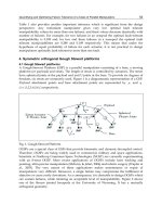
Fig. 3. Evolution of learning parameters according to noise level: a/ Reinforcement signal
and b/ corresponding error (m).
In order to identify the influence of uncertainty and noise reflecting low quality sensors, we have
considered four levels of noise with zero mean and standard deviation
V
n
of 0.2, 0.1, 0.05 and 0
(which corresponds to a deterministic reinforcement, r
k
 [0, 1]). Each trial has duration of 2000
steps and the bounds of the workspace are defined in Table I. In order to have a satisfying
convergence, we use the following learning rates
D
BP

= 0.01 for the BP units,
D
= 0.01 and
U
= 0.01
for the SRV units. In Fig. 3a/, the obtained reinforcement signals with the four noise standard
deviation levels are displayed as well as the corresponding deterministic error in Fig. 3b/. The
algorithm finds a satisfactory solution even if the curves are more irregular for large standard
deviations. We can also notice that the convergence is of the same order than the trial with
deterministic reinforcement attesting the model robustness to noise. Finally, a satisfactory solution
is obtained after a relatively low number of time steps.
At the beginning of the learning process the SRV units expected reinforcement is low and the
standard deviation parameter is high; thus the exploratory behavior is predominant. As training
proceeds, the mean of the SRV units Gaussian distribution is gradually shifted in such a direction
that the reinforcement increases. Consequently, the expected reinforcement increases and the
standard deviation decreases rapidly as well as the total error. Then, the exploitation behavior
becomes predominant and the hand configuration is slightly modified to optimize the solution.
X (m) Y (m) Z (m)
T
X (°)
T
Y (°)
T
Z (°)
min. value
-0.1 -0.1 0.15 -45 -45 -135
max. value
0.1 0.1 0.25 45 45 -45
Table 1. Search space bounds for the rectangular block five fingered grasp.
The results of the methods are constructed for grasps with different number of fingers and different

contact sets. MATLAB environment is used to solve the grasp planning problem (Pentium 4 HT
3.0Ghz, 512 ram, FSB 800 MHz). Three different grasps are considered in increasing number of
fingers : grasping a glass with three fingers (task 1) or four fingers (task 2) and grasping a videotape
with five fingers (task 3) (Fig. 4). For each task, twenty simulations are performed using the
proposed model. Only the deterministic reinforcement with a zero noise level is considered. The
results are summarized in Table 2. Results are displayed for each task in three columns. For task 1,
in the first and second ones are indicated the total error and the detail for each fingertip after 2 and 5
seconds of learning respectively. Finally, in the third column, the error after 2000 iterations is
displayed. For task 2, results are provided after 2 and 6 seconds of learning in first and second
columns and after 1000 iterations in the third one, for task 3, after 3 and 7 seconds and after 1000
iterations in column 1, 2 and 3 respectively. Average values
r standard deviation are provided.
Robotic Grasping: A Generic Neural Network Architecture 117
Task 1 Task 2 Task 3
Time (s) 2 5
18.5r12.3
2 6
14.8r5.2
3 7
18.9r3.2
Error (mm)
9.0r9.4 4.1r1.1 3.1r0.04 8.4r5.8 6.2r1.7 5.1r1.2 21.3r21.7 9.1r2.8 6.9r1.3
Thumb (mm)
2.6r1.4 1.9r0.8 1.5r0.7 3.4r2.9 2.5r1.3 2.1r0.9 7.0r9.8 3.7r1.5 3.0r0.9
Index (mm)
4.5r7.5 1.1r0.7 0.8r0.4 1.9r1.5 1.3r0.3 1.2r0.4 4.9r6.2 2.2r1.3 1.6r0.9
Middle (mm)
2.0r2.2 1.1r0.4 0.8r0.4 1.5r1.5 1.2r0.7 0.9r0.5 3.5r5.1 1.1r0.5 1.0r0.3
Ring (mm)
1.6r0.9 1.2r0.5 0.9r0.5 2.2r2.8 1.0r0.5 0.7r0.3

Pinky (mm)
3.7r7.4 1.2r1.0 0.7r0.3
Table 2. HCNN results.
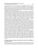
Finally, in Fig. 4, the obtained postures for task 1, 2 and 3 are displayed.
a/ Task 1 b/ Task 2 c/ Task 3
Fig. 4. Postures obtained by HCNN and optimization for the three tasks: a/ glass grasp with
3 fingers, b/ glass grasp with four fingers, c/ videotape grasp with five fingers.
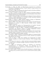
a/ b/
Fig. 5. Complete arm model, Model architecture when considering the arm and obstacles in
the environment.
6. Complete upper-limb posture definition with obstacle avoidance
In this section, a complete upper-limb is considered including an arm model associated with
the hand model described and used in the former section. The model capabilities are
extended by considering the presence of unknown obstacles in the environment (Rezzoug &
118 Mobile Robots, Towards New Applications
Gorce, 2006). The resolution principle is the same than the one used when considering the
hand only. Instead of the hand palm position, the arm joints configuration is considered as
input of the ACNN (Arm Configuration Neural Network) which replaces the HCNN of the
original model. Also, the arm forward model is used to compute the contact set in the frame
of the considered fingers as shown in Fig. 5b/.
6.1. Arm model
The model of the arm is composed of two segments and three joints (Fig. 5a/). The first
joint, located at the shoulder (gleno-humeral joint) has three degrees of freedom. The second
joint is located at the elbow and has one degree of freedom. Finally, the last joint, located at
the wrist, has three degrees of freedom. The final frame of the last segment defines the
orientation of the hand palm. According to this formulation, the arm posture is completely
defined by the joint angles vector q = [q
1
, q
2

, q
3
, q
4
, q
5
, q
6
, q
7
]
T
. The chosen model has 7
degrees of freedom (Fig. 5a/).
0 200 400 600 800 1000 1200 1400 1600 1800 2000
0.3
0.4
0.5
0.6
0.7
0.8
0.9
1
Iteration number
Reinforcement
R3, C > 0
R4, C = 2
R4, C = 3
R4, C = 4
R4, C = 5

R4, C = 6
R1 = 0.99
R2 = 0.495, C > 0
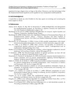
Fig. 6. Evolution of the reinforcements R
1
, R
2
, R
3
and R
4
relative to the iteration and collision
numbers.
6.2. Improving learning performances by shaping
In order to define a suitable reinforcement signal, two aspects of the performance have to be
taken into account. The first one evaluates the upper-limb positioning task while the second
is relative to collision avoidance. In the following, the different steps that conduct to the
definition of the appropriate reinforcement signal are described. Firstly, the positioning task
is evaluated. To do this, given the arm and fingers configuration, the actual position of the
fingertips is calculated using forward kinematics.
The simplest form of the reinforcement R
1
as used in section 4 gives a maximum penalty if
error E
k
is large and is given in (14) and recalled here (a is a positive real number):


1
1.

k
h
R
aE 
(20)
Starting from the definition of R
1
, the basic expression of the reinforcement signal that
incorporates collision avoidance behavior is given by:
Robotic Grasping: A Generic Neural Network Architecture 119
1
2
1
if no collision
if collision

/2
R
R
R


®
¯
(21)
In order to fulfill the secondary task i.e. collision avoidance, the reinforcement R
1
is
divided by two whenever a collision is detected. Therefore, even if the principal task is
accomplished with success the reinforcement is low due to the occurrence of a collision.

One can notice the simplicity of the incorporation of collision avoidance behavior in the
learning process. However, the criterion R
2
uses a somewhat crude strategy and the
results may not be as satisfying as expected. Indeed, the learning agent has to directly
discover the right strategy to satisfy two kinds of constraints at the same time. This is a
more complex task than arm positioning only.
In order to circumvent this difficulty, we propose to use a technique inspired from animal
training called shaping (Skinner, 1938). (Gullapalli, 1992) gave a nice definition of this
concept and applied it to the frame of reinforcement learning : “The principle underlying
shaping is that learning to solve complex problems can be facilitated by first learning to
solve simpler problems. … the behavior of a controller can be shaped over time by gradually
increasing the complexity of the task as the controller learns”.
To incorporate shaping in the learning procedure, the basic idea is to let the agent
learn the positioning task first and the collision avoidance behavior during a second
phase. To implement this, a reinforcement signal that gradually increases over time the
penalty due to collisions is defined. In this way, the agent can learn adequately the
first task and modify its behavior in order to achieve the second one. The
reinforcement value used in this case is the following (i is the current iteration number
and p the maximum number of iterations):

1
3
1
if no collision
if collision

/1 /
R
R

Rip


®

¯
(22)
If collisions occur, for the same value of R
1
, an increase of i conducts to an increase of the
denominator in (22) and consequently to a decrease of R
3
. If i = p, we can notice that R
3
= R
2
and that there is a gradual shift from R
1
(no penalty for collision) to R
2
(full penalty for
collision). This weaker definition of arm positioning with collision avoidance may be easier
to learn than direct collision avoidance as defined by R
2
. The evolution of R
3
with R
1
= 0.99
when collisions occur is displayed in Fig. 6.

The main drawback of R
3
is that the same penalty is applied whatever the number of
collisions. It may be easier to learn the task successfully if the learning agent can grade
differently two situations with different numbers of collision, giving more penalty to the
posture conducting to more collisions or interpenetrations. In order to solve this problem,
we define the reinforcement R
4
:


1
4
1
if no collision
if collision

/1 /
R
R
Rcip
E

°

®

°
¯
(23)

where c is the number of detected collision(s) or interpenetration(s) and
E
a positive real number.
Reinforcements R
3
and R
4
use the same strategy, except that R
4
takes into account the number
of collisions. Indeed, for the same value of R
1
, i and p, an increase of c conducts to an increase
of the denominator in (23) and therefore to a decrease of the reinforcement R
4
. If c = 1, we
notice that R
4
= R
3
. The evolution of R
4
, with different values of c is displayed in Fig. 6.
120 Mobile Robots, Towards New Applications
Fig. 7. Environments for the two grasping tasks.
6.3. Simulation results
The task to be performed is to grasp a cylinder with three fingers. Two different
environments are considered, the first one with a big obstacle between the arm and the
object and the second one with two obstacles (Fig. 7).
Reinforcement

R
1
R
2
R
3
R
4
Success 26 20 22 26
Positioning task 4 10 7 4 Causes
of failure
Collision 22 3 6 2
Mean iterations number 102 430 281 310
Standard deviation 126 271 259 245
Table 3. Simulation results for Task 1.
Reinforcement
R
1
R
2
R
3
R
4
Success 25 8 22 16
Positioning task 5 22 7 14 Causes
of failure
Collision 24 4 2 5
Mean iterations number 120 454 273 260
Standard deviation 161 266 228 223

Table 4. Simulation results for Task 2.
Thirty simulations are performed for each reinforcement and for each environment. The
weights of the ACNN are initialized with random values over the interval [-0.5, 0.5] and a
random arm configuration is chosen within the search space. We use the following values
for the parameters of the ACNN

D
BP
= 0.03,
D
SRV
= 0.03,
U
= 0.01, n
1
= 14, n
2
= n
3
= 20, n
4
= 7,
a = 1.5, p = 2000 and
E
= 0.25 The learning has to be completed for each task and
environment and is performed until a reinforcement greater than 0.99 is obtained or until
the maximum number of iterations is reached. A FCNN is constructed off line for each
finger before the simulations. Collision or interpenetration check is implemented with a two
steps scheme. Axis aligned bounding boxes are constructed for each element of the
environment to make a first check. If it is positive, the distance between any pair of solids

that are likely to collide is computed. This is done by minimizing the distance between any
pair of points on the surface of two elements of the scene modeled with superquadrics.
Robotic Grasping: A Generic Neural Network Architecture 121
In Tables 3 and 4 are displayed the obtained results. In the first row, the number of successes
is indicated for each reinforcement. This corresponds to the case where the reinforcement is
greater than 0.99. In the second and third rows is indicated the number of cases for which a
failure is due either to the positioning task or to collisions. Finally, for the successful cases,
the last two rows indicate the mean and standard deviation of the required number of
iterations to obtain a suitable reinforcement.
0 20 40 60 80 100 120 140 160 180
0
0.1
0.2
0.3
0.4
0.5
0.6
0.7
0.8
0.9
1
Iteration number
Reinforc ement
Reinforcement
Expected reinforcement
Standard deviation
0 50 100 150 200 250 300 350 400 450
0
0.1
0.2

0.3
0.4
0.5
0.6
0.7
0.8
0.9
1
Iteration number
Reinforcement
Reinforc ement
Expected reinforcement
Standard deviation
a/ b/
0 50 100 150 200 250 300
0
0.1
0.2
0.3
0.4
0.5
0.6
0.7
0.8
0.9
1
Iteration number
Reinforcement
Reinforcement
Expected reinforcement

Standard deviation
0 100 200 300 400 500 600
0
0.1
0.2
0.3
0.4
0.5
0.6
0.7
0.8
0.9
1
Iteration number
Reinforcement
Reinforcement
Expected reinforcement
Standard deviation
c/ d/
Fig. 8. Examples of learning parameters evolution for task 1 obtained with reinforcement a/
R
1
, b/ R
2
, c/ R
3
and d/ R
4
.
Reinforcement R

1
is used as a reference in order to demonstrate that the other
reinforcements R
2
, R
3
and R
4
have effectively an effect on collision avoidance.
The first observation is that the incorporation of collision avoidance behavior in the
reinforcement signal effectively leads to collision avoidance even if the positioning task is
not achieved. Using R
1
, 22 solutions out of 26 valid ones are obtained with collisions
between the upper limb and the environment for the first task and 24 out of 25 for the
second task. This number falls to 3, 6 and 2 for R
2,
R
3
and R
4
for the first task and 4, 2 and 5
for the second task respectively. Also, one can notice that there is an increase of the number
of successes when shaping is incorporated compared to the case where crude collision
avoidance reinforcement is used (R
2
). This is particularly obvious for the second task (8
successes with R
2
compared to 22 using R

3
). This suggests that the strategy of shaping
conducts to a higher number of valid solutions and therefore that the learning is enhanced.
122 Mobile Robots, Towards New Applications
In Fig. 8 is presented the evolution of the learning parameters using reinforcements R
1
, R
2
, R
3
and
R
4
. These curves give interesting information on the learning process. Indeed, using R
1
(Fig. 8a/),
the evolution of the expected reinforcement which is an internal parameter representing the
learning performance is “monotonic” and increasing, suggesting that the learning is performed in
one sequence and that there is a gradual shift from exploration to exploitation. This parameter
using R
2
(Fig. 8b/) has a far less regular evolution, denoting the increased difficulty to find a
solution due to the strict nature of R
2
. The evolution of R
3
and R
4
(Fig. 8c/ and 8d/) show the effect
of shaping. At the beginning of the learning, the expected reinforcement follows the same pattern

than using R
1
, i.e. a monotonic increasing function on average. As the number of iterations (NOI)
increases, the occurrence of collision(s) is more penalized and there is a decrease of the expected
reinforcement. This causes an augmentation of exploration evidenced by the augmentation of the
standard deviation (bold dashed curve). Then, taking advantage of the previous learning of the
positioning task, a solution is found that exhibits collision avoidance behavior. This is particularly
visible in Fig.9 where the evolution of the number of collisions using R
3
is shown (this case
corresponds to the results of Fig. 8c/). The agent has learned the first task without considering the
collisions. This is evidenced by the high number of collisions at the beginning of the learning.
Then, as the number of iterations increases this behavior is more penalized and using the previous
acquired knowledge the agent is able to learn the second aspect of the task (collision avoidance)
without a deterioration of the performance concerning the first aspect (i.e. grasping).
0 50 100 150 200 250 300
0
2
4
6
8
10
12
Iteration number
Number of collision(s)
Fig. 9. Evolution of the number of collision(s) using reinforcement R
3
.
To determine if the use of the different reinforcements has an effect on the NOI, a one way analysis
of variance (ANOVA) (Miller, 1997) on the number of iterations to complete the task is conducted.

A Bonferoni post-hoc test is used to perform multiple comparisons between means. The ANOVA
evidences a significant difference between four groups means (F(3, 161) = 14.33, p<0.0001). Also, the
post-hoc tests show a significant increase of the NOI using R
2
compared to the NOI using R
3
and R
4
(p<0.05). Also, a significant increase of the NOI using R
2
, R
3
and R
4
compared to the NOI using R
1
is
noticed (p<0.05). There is no significant difference between the NOI using R
3
and R
4
. These results
suggest that learning the positioning task is easier than the positioning task with collision avoidance
because, on average, more iterations are needed whatever the chosen reinforcement. Secondly, the
incorporation of shaping in the learning process reduces significantly the required number of
iterations to reach the goal. Finally, taking into account the number of collisions in the reinforcement
definition does not seem to improve significantly the learning performances. Therefore, among all
the reinforcement signals proposed in this study, we can consider that R
3
is the best one to perform

grasping posture definition with obstacles in the frame of the considered model. In Fig. 10, the
posture obtained to grasp a cylinder surrounded by 3 obstacles is shown.
Robotic Grasping: A Generic Neural Network Architecture 123
Fig. 10. Upper-limb posture to grasp a cylinder surrounded by 3 obstacles.
In the following section, a non anthropomorphic arm is considered. The method is slightly
modified to handle this case.
7. MANUS robot configuration definition
Several movements are needed to grasp an object: an approach phase during which the
end-effector is brought in the vicinity of the object followed by a grasping phase that
implies precise adjustments in order to orient properly the end-effector. This latter
phase can necessitate fine motions that are tedious if executed in manual control. To
reduce the difficulty of this task, we propose to automate partially the grasping phase
working in the vicinity of the arm configuration chosen by the user at the end of the
approach phase. More precisely, we define the angular configuration of the robot joints
in order to place the end-effector in an adequate configuration.
H
'
H
L
1
L
2
L
3
P
MANUS
Configuration
Neural
Network
MANUS

configuration at
time
t +1
MANUS
configuration
at time
t
End-effector
configuration
+
-
MANUS forward
kinematics
Position of the 2
points on the MANUS
end-effector
Position of the 2
target points on the
ob
j
ect
-
+
Reinforcement
computation
Fig. 11. a/ Degrees of freedom of the MANUS robot , b/ Model architecture.
7.1. Robot arm model
To define the mobile platform configuration 9 degrees of freedom have to be controlled (6 for the
MANUS and 3 for the mobile base). This task is made difficult due to the existence of an infinite
124 Mobile Robots, Towards New Applications

number of solutions to put the platform and the MANUS arm in a given configuration (Fig. 11a/).
In order to identify the object to be grasped, it is necessary to obtain information from a
camera. It seems important to define the needed amount of information to achieve the task
considering the trade off between efficacy and complexity.
During the grasping phase, two points defined on the end-effector of the MANUS arm
are associated with two points on the surface of the object. The goal of the grasping
task is to bring the MANUS arm in such a configuration that the two pairs of points
overlap. In this way, the constraints relative to the position as well as the orientation of
the end-effector are treated. Furthermore, the amount of the needed information is
limited to the position of four points in 3D. The corresponding model architecture is
displayed in Fig. 11b/.
The inputs of the model are the location of the two points of interest both on the MANUS
gripper and on the object and also the arm joint limits. The output is the mobile platform
configuration that optimizes a particular cost function composed of two parts:
1. A first term that insures that the axes defined by the two points on the surface of the
object and on the MANUS gripper are collinear.
2. A second term to minimize the distance between each couple of points.
The first part evaluates the orientation of the gripper relative to the object. Its expression is
given in (24).
1
R 
Gripper Object
nn
(24)
n
Gripper
is the unit vector aligned with the axe defined by the two points on the MANUS
gripper and n
Object
is the unit vector defined by the two points on the object. The maximum

value of R
1
is reached when the two vectors are collinear, then R
1
= 1. On the other hand,
when the two vectors are orthogonal R
1
= 0.
The second part of the cost function evaluates the distance between the couples of points. It
is defined as following:


2
1tanh
R
d 
(25)
where

12
min ,ddd
(26)
With
1
d 
Object Gripper Object Gripper
11 22
X-X X-X
(27)
2

d 
Object Gripper Object Gripper
21 12
X-X X-X
(28)
Object
i
X
and
Gripper
i
X
(i = 1, 2) represent the 3D position of the points attached to the object and to
the gripper in. d represents the minimum of the summed distances between the couple of
points on the gripper and the object.
The function tanh insures that R
2
lies in the interval [0, 1]. R
2
is minimum if d is high and
maximum (R
2
= 1) if d = 0. Combining the two criteria, the cost function R (29) is obtained.
12
2
R
R
R


(29)
Robotic Grasping: A Generic Neural Network Architecture 125
a/ b/
Fig. 12. a/Criterion evolution and b/simulated MANUS robot configuration.
7.2. Simulation results
In this section, simulation results are presented. The grasp of a cube placed at different
locations is considered. The contact points location and the position of the object are known
and considered as input data. The arm starts from a random position within its workspace.
The graphs of Fig. 12a/ displaying the evolution of the learning criteria R
1
, R
2
and R during
learning show the ability of the model to discover the adequate configuration while
satisfying orientation and position constraints. Also, to evaluate the performances of the
method over a workspace, 30 simulations are performed for each of 64 object positions
equally distributed in a 0.6 m x 0.6 m x 1m workspace. The obtained mean d (3) is 9.6 r 4.1
mm. For one situation, the platform configuration is shown in Fig. 12b/.
8. Conclusion
In this chapter, a new model was proposed to define the kinematics of various robotic
structures including an anthropomorphic arm and hand as well as industrial or service
robots (MANUS). The proposed method is based on two neural networks. The first one
is dedicated to finger inverse kinematics. The second stage of the model uses
reinforcement learning to define the appropriate arm configuration. This model is able
to define the whole upper limb configuration to grasp an object while avoiding
obstacles located in the environment and with noise and uncertainty. Several
simulation results demonstrate the capability of the model. The fact that no
information about the number, position, shape and size of the obstacles is provided to
the learning agent is an interesting property of this method. Another valuable feature
is that a solution can be obtained after a relatively low number of iterations. One can

consider this method as a part of a larger model to define robotic arm postures that
tackles the “kinematical part” of the problem and can be associated with any grasp
synthesis algorithm. In future work, we plan to develop algorithms based on
unsupervised learning and Hopfield networks to construct the upper-limb movement.
In this way, we will be able to generate an upper-limb collision free trajectory in joint
coordinate space from any initial position to the collision free final configuration
obtained by the method described in this article.
126 Mobile Robots, Towards New Applications
9. References
Bard, C.; Troccaz, J. & Vercelli, G. (1991). Shape analysis and hand preshaping for grasping,
Proceedings of the 1991 IEEE/RSJ Int. Workshop on Intelligent Robots and Systems, pp
64-69, 1991, Osaka, Japan
Becker, M.; Kefalea, E.; Mael, E.; von der Malsburg, C.; Pagel, M.; Triesch, J.; Vorbruggen, J.
C.; Wurtz, R. P. & Zadel, S. (1999). GripSee: A gesture-controlled robot for object
perception and manipulation. Autonomous Robots, Vol. 6, No 2, 203-221
Bekey, G. A.; Liu, H.; Tomovic, R. & Karplus, W. J., (1993). Knowledge-based control of
grasping in robot hands using heuristics from human motor skills. IEEE
Transactions on Robotics and Automation, Vol. 9, No 6, 709-721
Borst, C.; Fischer, M. & Hirzinger, G. (2002). Calculating hand configurations for precision
and pinch grasps, Proceedings of the 2002 IEEE Int. Conf. on Intelligent Robots and
Systems, pp 1553-1559, 2002, Lausanne, Suisse
Coehlo, J. A. & Grupen, R. A. (1997). A control basis for learning multifingered grasps.
Journal of Robotic Systems, Vol. 14, No. 7, 545-557
Cutkosky, M. R. (1989). On grasp choice, grasp models, and the design of hands for
manufacturing tasks. IEEE Transactions on Robotics and Automation, Vol.5, 269-279
Doya, K., (2000). Reinforcement learning in continuous time and space. Neural Computation,
Vol. 12, 243 - 269
Ferrari, C. & Canny, J. (1992). Planning optimal grasps, Proceedings of the 1992 IEEE Int. Conf.
on Robotics and Automation, pp 2290-2295, 1992, Nice, France
Gorce, P. & Fontaine J. G. (1996). Design methodology for flexible grippers. Journal of

Intelligent and Robotic Systems, Vol. 15, No. 3, 307-328
Gorce, P. & Rezzoug, N. (2005). Grasping posture learning from noisy sensing information
for a large scale of multi-fingered robotic systems. Journal of Robotic Systems, Vol.
22, No. 12, 711-724.
Grupen, R., & Coelho, J. (2002). Acquiring State form Control Dynamics to learn grasping policies
for Robot hands. International Journal on Advanced Robotics, Vol. 15, No. 5, 427-444
Guan, Y. & Zhang, H. (2003). Kinematic feasibility analysis of 3-D multifingered grasps.
IEEE Transactions on Robotics and Automation, Vol. 19, No. 3, 507-513
Gullapalli, V. (1990). A stochastic reinforcement learning algorithm for learning real valued
functions. Neural Networks, Vol. 3, 671-692
Gullapalli, V. (1992) Reinforcement learning and its application to control. PhD Thesis, University
of Massachusetts, MA, USA
Gullapalli, V. (1995). Direct associative reinforcement learning methods for dynamic
systems control, Neurocomputing, Vol. 9, 271-292
Iberall, T. (1997). Human prehension and dexterous robot hands. International Journal of
Robotics Research, Vol. 16, No 3, 285-299
Iberall, T.; Bingham, G. & Arbib, M. A. (1986). Opposition space as a structuring concept for the
analysis of skilled hand movements. Experimental Brain Research, Vol. 15, 158-173
Jeannerod, M. (1984). The timing of natural prehension. Journal of Motor Behavior, Vol. 13, No
3, 235-254
K. Pook and Ballard, Recognizing teleoperated manipulations, Proceedings of the 1996 IEEE
Int. Conf. on Robotics and Automation , pp 578-583, 1993, Atlanta, GE, USA
Kaelbling, L. P.; Littman, M. L. & Moore, A. W. (1996). Reinforcement learning: a survey.
Journal of Artificial Intelligence Research, Vol. 4, 237-285
Robotic Grasping: A Generic Neural Network Architecture 127
Kang, S. B. & Ikeuchi, K., (1997). Toward automatic robot instruction from perception -
Mapping human grasps to manipulator grasps. IEEE Transactions on Robotics and
Automation, Vol 13, No 1, 81-95
Kerr, J. & Roth, R. (1986). Analysis of multifingered hands. The International Journal of
Robotics Research, Vol. 4, 3-17

Kuperstein, M. & Rubinstein, J. (1989). Implementation of an adaptative controller for
sensory-motor condition, in: Connectionism in perspective, Pfeiffer, R.; Schreter, Z.;
Fogelman-Soulie, F. & Steels, L., (Ed.), pp. 49-61, Elsevier Science Publishers, ISBN
0-444-88061-5 , Amsterdam, North-Holland
Lee, C. & Xu, F. Y., (1996). Online, Interactive learning of gestures for human/robot
interface, Proceedings of the 1996 IEEE Int. Conf. on Robotics and Automation, pp 2982-
2987, 1996, Minneapolis MI, USA
Miller, A. T. & Allen, P. K. (1999). Examples of 3D grasps quality measures, Proceedings of the 1999
IEEE Int. Conf. on Robotics and Automation, pp. 1240-1246, 1999, Detroit MI, USA
Miller, A. T.; Knoop, S.; Allen, P. K. & Christensen, H. I. (2003). Automatic grasp planning
using shape primitives, Proceedings of the 2003 IEEE Int. Conf. on Robotics and
Automation, pp. 1824-1829, 2003, Taipei Taiwan
Miller, R.G., (1997). Beyond Anova, Basics of applied statistics, Chapman & Hall/CRC, Boca
Raton, FL, USA
Mirtich, B. & Canny, J. (1994). Easily computable optimum grasps in 2D and 3D, Proceedings
of the 1994 IEEE Int. Conf. on Robotics and Automation, pp 739–747, 1994, San Diego
CA, USA
Moussa M. A. & Kamel, M. S. (1998). An Experimental approach to robotic grasping using a
connectionist architecture and generic grasping functions. IEEE Transactions on
System Man and Cybernetics, Vol. 28, 239-253
Napier, J.R. (1956). The prehensile movements of the human hand. Journal of Bone and Joint
Surgery, Vol. 38, 902-913
Nguyen, V. (1986). Constructing force-closure grasps, Proceedings of the 1986 IEEE Int. Conf.
on Robotics and Automation, pp 1368-1373, 1986, San Francisco CA , USA
Oyama, E. & Tachi, S. (1999). Inverse kinematics learning by modular architecture neural
networks, Proceedings of the 1999 IEEE Int. Joint Conf. on Neural Network, pp 2065-
2070, 1999, Washington DC, USA
Oyama, E. & Tachi, S. (2000). Modular neural net system for inverse kinematics learning,
Proceedings of the 2000 IEEE Int. Conf. on Robotics and Automation, pp 3239-3246,
2000, San Francisco CA, USA

Pelossof, R.; Miller, A.; Allen, P. & Jebara, T. (2004). An SVM learning approach to robotic
grasping, Proceedings of the 2002 IEEE Int. Conf. on Robotics and Automation, pp. 3215-
3218, 2004, New Orleans LA, USA
Rezzoug, N. & Gorce, P. (2001). A neural network architecture to learn hand posture
definition, Proceedings of the 2001 IEEE Int. Conf. on Systems Man and Cybernetics, pp.
3019-3025, 2001, Tucson AR, USA
Rezzoug, N. & Gorce, P. (2006). Upper-limb posture definition during grasping with task
and environment constraints. Lecture Notes in Computer Science / Artificial
Intelligence, Vol. 3881, 212–223.
Saito, F. & Nagata, K. (1999). Interpretation of grasp and manipulation based on grasping
surfaces, Proceedings of the 1999 IEEE Int. Conf. on Robotics and Automation, pp 1247-
1254, 1999, Detroit MI, USA
128 Mobile Robots, Towards New Applications
Skinner, B.F. (1938). The behavior of organisms : An experimental analysis, D Appleton century,
New York, USA
Sutton, R. S. & Barto, A.G. (1998). Reinforcement learning, MIT Press, Cambridge, MA
Sutton, R. S. (1988). Learning to predict by the methods of temporal difference. Machine
Learning, Vol. 3, 9-44
Taha, Z.; Brown, R. & Wright, D. (1997). Modelling and simulation of the hand grasping
using neural networks. Medical Engineering and Physiology, Vol. 19, 536-538
Tomovic, R.; Bekey, G. A. & Karplus, W. J. (1987). A strategy for grasp synthesis with
multifingered hand, Proceedings of the 1987 IEEE Int. Conf. on Robotics and
Automation, pp. 83-89, 1987, Raleigh NC, USA
Uno, Y.; Fukumura, N.; Suzuki, R. & Kawato, M. (1995). A computational model for
recognizing objects and planning hand shapes in grasping movements. Neural
Networks, Vol. 8, 839-851
Watkins, C. J. C. H., (1989). Learning form delayed reward. PhD thesis, Cambridge University,
MA, USA
Wheeler, D., Fagg, A. H. & Grupen, R. (2002). Learning prospective Pick and place behavior,
Proceedings of the 2002 IEEE/RSJ Int. Conf. on Development and Learning, pp 197-202,

2002, Cambridge MA, USA
Wren, D. O. & Fisher, R. B. (1995). Dextrous hand grasping strategies using preshapes and
digit trajectories, Proceedings of the 1995 IEEE Int. Conf. on Systems, Man and
Cybernetics, pp. 910-915, 1995, Vancouver, Canada
7
Compliant Actuation of Exoskeletons
1
H. van der Kooij , J.F. Veneman, R. Ekkelenkamp
University of Twente
the Netherlands
1. Introduction
This chapter discusses the advantages and feasibility of using compliant actuators in
exoskeletons. We designed compliant actuation for use in a gait rehabilitation robot. In such
a gait rehabilitation robot large forces are required to support the patient. In case of post-
stroke patients only the affected leg has to be supported while the movement of the
unaffected leg should not be hindered. Not hindering the motions of one of the legs means
that mechanical impedance of the robot should be minimal. The combination of large
support forces and minimal impedances can be realised by impedance or admittance control.
We chose for impedance control. The consequence of this choice is that the mass of the
exoskeleton including its actuation should be minimized and sufficient high force
bandwidth of the actuation is required. Compliant actuation has advantages compared to
non compliant actuation in case both high forces and a high force tracking bandwidth are
required. Series elastic actuation and pneumatics are well known examples of compliant
actuators. Both types of compliant actuators are described with a general model of
compliant actuation. They are compared in terms of this general model and also
experimentally. Series elastic actuation appears to perform slightly better than pneumatic
actuation and is much simpler to control. In an alternative design the motors were removed
from the exoskeleton to further minimize the mass of the exoskeleton. These motors drove
an elastic joint using flexible Bowden cables. The force bandwidth and the minimal
impedance of this distributed series elastic joint actuation were within the requirements for

a gait rehabilitation robot.
1.1 Exoskeleton robots
Exoskeletons are a specific type of robots meant for interaction with human limbs. As the
name indicates, these robots are basically an actuated skeleton-like external supportive
structure. Such robots are usually meant for:
• Extending or replacing human performance, for example in military equipment
(Lemley 2002), or rehabilitation of impaired function (Pratt et al. 2004),
• Interfacing; creating physical contact with an illusionary physical environment or
object; these haptic devices are usually referred to as kinaesthetic interfaces. Possible
applications appear for example in gaming and advanced fitness equipment, or in
1
Parts of this chapter have been published in The International Journal of Robotics Research 25, 261-281
(2006) by Sage Publications Ltd, All rights reserved. (c) Sage Publications Ltd
130 Mobile Robots, Towards New Applications
creating ‘telepresence’ for dealing with hazardous material or difficult circumstances
from a safe distance (Schiele and Visentin 2003).
• Training human motor skills, for example in the rehabilitation of arm functionality
(Tsagarakis and Caldwell 2003) or gait (Colombo et al. 2002) after a stroke.
Every typical application has specific demands from a mechatronical design viewpoint. Robots in
interaction with human beings should be perceived as compliant robots, i.e. humans should be
able to affect the robots motions. In other words, the soft robots should have an impedance (or
admittance) control mode, sensing the actions of the human beings. Since the impedance or
admittance control does not need to be stiff but compliant we can use compliant actuators. An
advantage of compliant actuators is that the impedance at higher frequencies is determined by the
intrinsic compliance of these actuators. For non compliant actuators the impedance for frequencies
higher than the control bandwidth is determined by the reflected motor mass. In general, the
impedance of the reflected motor mass will be much higher than intrinsic compliance of compliant
actuators, especially when the needed motor torques and powers will be high. The advantage of
compliant actuators is that they not only have a favourable disturbance rejection mode (through
the compliance), but also have sufficient force tracking bandwidth. The compliant actuators

discussed in this article were evaluated for use in an exoskeleton for gait training purpose, but
might find wider application. First of all the specific application will be described, followed by
models and achieved performance of the actuators.
1.2 Context: a gait rehabilitation robot
We are developing a LOwer-extremity Powered ExoSkeleton (LOPES) to function as a gait
training robot. The target group consists of patients with impaired motor function due to a
stroke (CVA). The robot is built for use in training on a treadmill. As a ‘robotic therapist’
LOPES is meant to make rehabilitation more effective for patients and less demanding for
physical therapists. This claim is based on the assumptions that:
• Intensive training improves both neuromuscular function and all day living
functionality(Kwakkel et al. 2002; Kwakkel et al. 2004),
• A robot does not have to be less effective in training a patient than a therapist
(Reinkensmeyer et al. 2004; Richards et al. 2004),
• A well reproducible and quantifiable training program, as is feasible in robot assisted
training, would help to obtain clinical evidence and might improve training quality
(Reinkensmeyer et al. 2004).
The main functionality of LOPES will be replacing the physiotherapists’ mechanical
interaction with patients, while leaving clinical decisions to the therapists’ judgment. The
mechanical interaction mainly consists of assistance in leg movements in the forward and
sideward direction and in keeping balance.
Within the LOPES project, it has been decided to connect the limbs of the patient to an
'exoskeleton' so that robot and patient move in parallel, while walking on a treadmill. This
exoskeleton (Fig. 1) is actuated in order to realize well-chosen and adaptable supportive actions
that prevent fail mechanisms in walking, e.g. assuring enough foot clearance, stabilizing the knee,
shifting the weight in time, et cetera. A general aim is to allow the patient to walk as unhindered as
possible, while offering a minimum of necessary support and a safe training environment.
Depending on the training goals, some form of kinaesthetic environment has to be added. This
constitutes the main difference between LOPES and the commercially available gait-trainers.
Those are either position controlled devices that overrule the patient and/or allow only limited
motions due to a limited number of degrees of freedom, and/or are not fully actuated (Hesse et al.

Compliant Actuation of Exoskeletons 131
2003). Position controlled devices omit the training challenges of keeping balance and taking
initiative in training. More research groups have recognized this shortcoming (Riener et al. 2005).
In the control design of the exoskeleton in general two 'extreme' ideal modes can be defined, that
span the full range of therapeutic interventions demanded in the LOPES project. In one ideal mode,
referred to as 'robot in charge', the robot should be able to enforce a desired walking pattern, defined
by parameters like walking speed and step-length. This can be technically characterized as a high
impedance control mode. In the other ideal mode, referred to as 'patient in charge' the robot should
be able to follow the walking patient while hardly hindering him or her. This can be technically
characterized as a low impedance control mode. An intelligent controller or intervention by a
therapist then can adjust the actual robot behaviour between these high and low impedance modes.
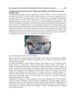
Fig. 1. Design of LOPES. Left: DoFs of the exoskeleton that are actuated. Other DoFs are left free
(ankle knee ab/aduction) or constrained (hip and knee endo/exorotation). middle: schematic
drawing of the construction for connecting the exo-skeleton to the fixed world consisting of height
adjustable frame (1), two sets of parallel bars with carriages for the for-/backward (2) and
sideways (3) motion that are both actuated, and a parallogram with weight compensation the
allows for vertical pelvic motion as occurs while walking. Right: photo of LOPES.
1.3 Impedance- versus admittance-controlled interactive robots
Many issues arising in the design of interactive neuro-rehabilitation robots are similar to
those appearing the field of haptic, or more precise: kinaesthetic robotics (Brown et al. 2003).
The characteristic feature of these robots is the bi-directionality of being able to both 'read
from' and 'write to' a human user (Hayward and Astley 1996). Such robots are in general
meant to display virtual objects or a virtual environment to a user. This user then can
interact with a virtual or distant ‘world’ in a mechanically realistic way.
In contrast, interactive neuro-rehabilitation robots are meant to operate in between both
stated modes of ‘robot in charge’ and ‘patient in charge’, acting as a ‘robotic therapist’; not
to display virtual objects as realistic as possible. Another difference, specific for limb-
guiding exoskeletons, is that a kinaesthetic display usually has an end-effector that displays
the information at one location on the robot, while an exoskeleton necessarily interacts at
several points with human limbs as it is connected in parallel to the limbs. This implies that

not only an end-effector force is important, but all ‘internal’ torques over all actuated joints.
This all makes it necessary to first select the optimal basic control outline for this kind of
robot, as different outlines imply different robot construction and actuator demands.
In general there are two basic ways to realize a kinaesthetic display (Adams and Hannaford
2002); impedance-control-based that is 'measure position and display force' (Fig. 2 left) and
admittance-control-based (Fig. 2 right) that is 'measure force and display position', although
132 Mobile Robots, Towards New Applications
hybrid forms exist. The important difference is that in impedance-control the quality of the
display will depend on the accuracy of the position sensors and the bandwidth and accuracy of
the force servos, and in case of admittance-control on the accuracy of the force sensors and the
bandwidth and accuracy of the position servo. The bandwidth of the mentioned servos will
depend on both the robot construction and the actuators. The choice between high performance
force servo quality and high performance position servo quality puts specific demands on the
robot construction and actuation. This choice has to be made even if a hybrid control architecture
with both position and force sensing is used. To make clear what this choice basically is about it
can also be presented as the choice between a lightweight (and flexible) uncompensated
construction and a rigid (and heavy) controller-compensated construction.
Fig. 2. Basic outline of an impedance-control (left) and admittance-control based rehabilitation robot.
A fundamental limitation of impedance control is that in each specific controlled degree of
freedom (or ‘dof’) the dynamical behavior of the robot construction in this ‘dof’ appears in the
force transfer (‘device dynamics’) (Fig. 1). It can only be compensated for in case of a proper
dynamical predictive model, and proper measurements of position and velocity for stiffness and
friction compensation respectively. Mass compensation is possible to a small extent only, by
adding a force or acceleration feedback loop (resulting in a hybrid control architecture). Best
results within an impedance-control architecture are obtained using a lightweight, low friction
construction and a low impedance actuator, so that the intrinsic mechanical impedance of the
device is kept low. Impedance controlled robots typically display ‘low-forces’ and lack
performance in kinaesthetic display of high inertia and high stiffness. (Linde and Lammertse
2003). This is not essential in gait-rehabilitation as no stiff contacts or large inertias have to be
displayed, although relatively high forces certainly appear.

An admittance control scheme, on the other hand, demands for a high positioning bandwidth,
and therefore for high(-er) power actuators and a stiff construction without backlash (Linde and
Lammertse 2003). A limitation of admittance control is that the display of low stiffness (‘free
motion’) can become instable, especially in case of a rather stiff user, because of the high control
gains needed in this case. Another limitation is that admittance can only be controlled at the
location(-s) of the force sensors. The construction will display its intrinsic impedance at other
locations, since the interaction behaviour there cannot be influenced by the controller without
force sensing. This might pose a problem for application in neuro-rehabilitation, because of the
possible safety threat (for instance for the therapist). The robot will not react to mechanical
interactions that by-pass the force sensors. This is all the more important as with admittance
control actuators and construction will be considerably heavier.
Summarizing, compared to general kinaesthetic devices a less critical stiffness- and mass-
display is demanded and movements are relatively slow. An admittance controlled system
imply larger safety threats due to the higher required actuator power, rigidity and inertia of
the robot and is less stable when a low stiffness is displayed. Considering all this we choose
an impedance-control based design strategy for our exoskeleton. An important advantage is
also that the programmed dynamical behaviour will be available everywhere on the
construction, that is, in every actuated degree of freedom.
Compliant Actuation of Exoskeletons 133
Impedance control implies that the actuators should be perfect force sources, or, realistically, low-
impedance, high precision force sources (in contrast with position sources that would be needed
for admittance control). The construction therefore should be lightweight, although being able to
bear the demanded forces, and should contain less friction. Fig. 3 shows the robot control outline
for one degree of freedom (DoF) that is impedance controlled.
Fig. 3. Schematic control outline for one degree of freedom. The inner loop (shaded area) assures
that the actuator acts as a pure force source. The outer loop (impedance controller) sets the force
reference based on desired impedance and actual displacement. The load reflects the
robot/human-combination dynamics in the considered DoF. In case the actuator is compliant the
load displacement directly influences the force output. Symbols: x
load

– position load; F – force;
F
dis
– external force disturbance;n
F
– force sensor noise; n
x
– position sensor noise.
1.4 Advantages of compliant actuation in impedance controlled devices with ‘high
force’ demands
As addressed by Robinson (Robinson 2000), commonly used actuators are poor force
actuators, even if in many theoretic approaches actuators are supposed to be pure force
sources. For small robots common brushless DC motors in combination with cable drives,
usually suffice, as for example used in the WAM-arm (Townsend and Guertin 1999), a
haptic device. In general, actuators with high force and high power density typically have a
high mechanical output impedance due to necessary power transmission (e.g. geared EM
motors) or the nature of the actuator (e.g. hydraulics). These actuators do not have a large
force tracking bandwidth in case high forces have to be displayed.
The solution suggested by Robinson, and several others (Morrell and Salisbury 1998;
Robinson 2000; Bicchi et al. 2001; Sugar 2002; Zinn et al. 2004) is to decouple the dynamics of
the actuator and the load, by intentionally placing a compliant element, e.g. a spring,
between both. The actuator can then be used in a high gain position control loop, resulting
in an accurate control of spring deflection and resulting force, while compensating the
internal dynamics of the actuator. The advantage of a compliant element is that it not only
filters friction and backlash and other non-idealities in transmission drives from the force
output, but also that it absorbs shock loadings from the environment.
An alternative way of realizing such a compliant actuator is to use a pneumatic actuator,
which is compliant due to the physics of air. The most straightforward way is by using a
134 Mobile Robots, Towards New Applications
double-acting cylinder, but also an antagonistic pair of fluidic muscles achieves a double

acting system (Ferris et al. 2005). Instead of measuring spring-deflection, pressure
measurements can be used as indirect force measurement.
Mechanical compliance in the actuation does not offer its advantages without costs. The lower the
stiffness, the lower the frequency with which larger output forces can be modulated. This is
caused by saturation effects that limit the maximal achievable acceleration of the motor mass and
spring length, or by the limited fluid flows for given certain pressures. A limited ‘large force
bandwidth’ decreases in turn the performance in terms of positioning-speed and -accuracy. A
careful design and trade-off is needed to suit such actuators for a typical application.
As mentioned by Robinson, it is not yet obvious how to select the proper elastic actuator for
a certain application. His general models appeared to be useful for predicting behaviour of a
series elastic actuator configuration, but do not clarify what the limitations of several
implementations of elastic actuators are. He suggested that important parameters would be
the force and power density levels of the specific configuration. To make a proper
comparison between series elastic actuators and pneumatic elastic actuators, the latter will
have to be described in similar parameters as the first. Once this is achieved the question of
the limits and (dis-)advantages of both types of elastic actuation can be addressed.
1.5 Actuator demands in an impedance controlled rehabilitation robot
Impedance control implies specific demands for the actuators in the robot. They should:
- be ‘pure’ (low impedance) force sources
- add little weight and friction to the moving robot construction in any degree of
freedom, not only the specific degree of freedom actuated by the considered actuator
- be safe, even in case of failure
- allow fast adjustment to the individual patient’s sizes
- be powerful enough for the ‘robot in charge’ task.
More specific, we decided that the actuators should be able to modulate their output force with
12 Hz for small forces, and 4 Hz for the full force range. Maximum joint moments differ per joint,
and range from 25 to 60 Nm. Joint powers range up to 250 Watt per joint. These numbers were
based on study of the human gait cycle and the motion control range of a human therapist. An
analysis of a nominal gait cycle (Winter 1991) was studied to obtain maximal needed torques,
speeds and powers during walking, and general data on human motor control were studied to

estimate maximum expected force-control speed and accuracy of a physical therapist.
The resulting actuator bandwidths are typically lower, and the forces typically higher than in the
specifications of common kinaesthetic devices which are intended for haptic display of a virtual
object, but not to assist humans. Actuators usually selected for kinaesthetic devices are either
heavy (like direct drive electro-motors) or poor force actuators (like geared DC motors).
We evaluated different compliant actuators. A series elastic actuator and a pneumatic cylinder
were dimensioned to meet the required demands state above. Both type of actuators were
modelled, evaluated and compared with each other. Next, we also designed and evaluated a
new type of series actuator. To minimize the mass of the exoskeleton we disconnected the motor
from the exoskeleton and connected the motor with the elastic joints through Bowden cables.
2. A framework for compliant actuation
In this paragraph we first will derive a general model for compliant actuators. Next we will
put pneumatic and series elastic actuation into this general framework.
Compliant Actuation of Exoskeletons 135
2.1 General model of a compliant actuator
The first step in comparing compliant actuators is a general model (Fig. 4) that is detailed and
flexible enough to describe the essential behaviour of any kind of compliant actuator, in this case
both a series elastic actuator based on a brushless DC motor, and a double-acting pneumatic
cylinder. The basic element of such an actuator is its elastic element or elasticity that we define as
it intrinsic stiffness (K
s
). Furthermore it should contain a motor block that modulates spring
length or the force. A last important factor is the friction after the elastic element, as this (usually
complex) friction can hardly be compensated for by a controller. It appears from this scheme that
the actual load influences the force tracking performance, as the load displacement (x
load
) is an
input to the system. With this general model, parts can be modelled as complex as seems
necessary, or as complex as availability of system parameters allows for. All parameters should
of course be transformed to the output axis domain, to fit in the general model.

Hint
K
s
Fref
x
load
xint Fact+
-
+
-
x
s
Cint
Ferror ucontrol
Hfrict
+
+
Fs
Ffrict
Fig. 4. General model of a compliant actuator, (fitting in the shaded area of Fig. 3), consisting of a
controlled (with controller C
int
) internal position source (H
int
) a compliant element with (variable)
stiffness (K
s
) and a (variable) friction model (H
frict
). These subsystems are possibly non-linear. The

force over the spring element F
s
is the actually controlled force, because it is intrinsically measured.
In case the real output force F
act
is measured, this measurement should be used for control, so that
also the friction can be compensated. Position variables concerning the elastic element are: x
int
position of the internal side, x
load
is the load position, x
s
the spring length. F
ref
is the desired
reference force, F
frict
the (external) friction force, whose sign depends on the motion direction.
For every kind of compliant actuator the H
int
forward path transfer function (H
fp
) has to be
determined. For practical reasons (so that the transfer can be directly measured) the stiffness
is included in the transfer. The load impedance is taken infinite corresponding to a fixed
load. The H
frict
is not included as the linear damping in this transfer function can not be
measured since the load is fixed:
()

act
fp s int s
control
load
,()
F
H
KHK
u
Z
ωω
==
=∞
(1)
By applying feedback control the force tracking transfer function for fixed load conditions becomes:
()
act int int s
force s
ref int int s
load
()
,
1()
F
CH K
HK
F
CH K
Z
ω

ω
ω
==
+
=∞
(2)
The mechanical output impedance of this controlled actuator is:
)(1
),(
intint
ω
ω
HCK
K
x
F
KZ
s
s
load
act
s
+
−
==
(3)
This already shows that, if the C
int
.
H

int
-gain falls off at higher frequencies, the impedance
will become equal to -K
s
at those frequencies. It also shows that the mechanical output