Tribology in Machine Design 2009 Part 2 pot
Bạn đang xem bản rút gọn của tài liệu. Xem và tải ngay bản đầy đủ của tài liệu tại đây (709.13 KB, 30 trang )
18
Tribology
in
machine
design
where
A
T
is the
real
area
of
contact,
r
max
denotes
the
ultimate shear strength
of
a
material
and
T
S
is the
average interfacial
shear
strength.
2.6.
Energy
dissipation
In a
practical engineering situation
all the
friction
mechanisms, discussed
so
during
friction
far on an
individual basis, interact with each other
in a
complicated way.
Figure
2.5 is an
attempt
to
visualize
all the
possible steps
of
friction-induced
energy
dissipations.
In
general,
frictional
work
is
dissipated
at two
different
locations within
the
contact zone.
The first
location
is the
interfacial
region
characterized
by
high rates
of
energy dissipation
and
usually associated
with
an
adhesion model
of
friction.
The
other
one
involves
the
bulk
of the
body
and the
larger volume
of the
material subjected
to
deformations.
Because
of
that,
the
rates
of
energy dissipation
are
much lower. Energy
dissipation during ploughing
and
asperity deformations takes place
in
this
second location.
It
should
be
pointed out, however, that
the
distinction
of
two
locations
being completely independent
of one
another
is
artificial
and
serves
the
purpose
of
simplification
of a
very complex problem.
The
various
processes
depicted
in
Fig.
2.5 can be
briefly
characterized
as
follows:
(i)
plastic deformations
and
micro-cutting;
(ii)
viscoelastic deformations leading
to
fatigue
cracking
and
tearing,
and
subsequently
to
subsurface excessive heating
and
damage;
(iii)
true sliding
at the
interface leading
to
excessive heating
and
thus
creating
the
conditions favourable
for
chemical degradation
(polymers);
(iv)
interfacial shear creating transferred
films;
(v)
true sliding
at the
interface
due to the
propagation
of
Schallamach
waves
(elastomers).
Figure
2.5
2.7.
Friction
under
Complex
motion conditions
arise
when,
for
instance,
linear sliding
is
complex
motion
combined with
the
rotation
of the
contact
area
about
its
centre (Fig. 2.6).
conditions
Under such conditions,
the
frictional force
in the
direction
of
linear motion
Basic
principles
of
tribology
19
is
not
only
a
function
of the
usual variables, such
as
load, contact
area
diameter
and
sliding velocity,
but
also
of the
angular velocity. Furthermore,
there
is an
additional
force
orthogonal
to the
direction
of
linear motion.
In
Fig. 2.6,
a
spherically ended
pin
rotates about
an
axis normal
to the
plate
with
angular velocity
co
and the
plate translates with linear velocity
V.
Assuming
that
the
slip
at the
point within
the
circular
area
of
contact
is
opposed
by
simple Coulomb
friction,
the
plate
will
exert
a
force
T dA in the
direction
of the
velocity
of the
plate relative
to the pin at the
point under
consideration.
To find the
components
of the
total frictional force
in the x
and y
directions
it is
necessary
to sum the
frictional
force
vectors,
x dA,
over
the
entire contact area
A.
Here,
i
denotes
the
interfacial shear strength.
The
integrals
for
the
components
of the
total frictional
force
are
elliptical
and
must
be
evaluated numerically
or
converted into tabulated
form.
Figure
2.6
2.8.
Types
of
wear
and
Friction
and
wear
share
one
common feature, that
is,
complexity.
It is
their
mechanisms
customary
to
divide wear occurring
in
engineering practice into
four
broad
general classes,
namely:
adhesive wear,
surface
fatigue wear, abrasive wear
and
chemical wear. Wear
is
usually associated with
the
loss
of
material
from
contracting bodies
in
relative motion.
It is
controlled
by the
properties
of
the
material,
the
environmental
and
operating conditions
and the
geometry
of
the
contacting bodies.
As an
additional factor influencing
the
wear
of
some materials, especially certain organic polymers,
the
kinematic
of
relative
motion within
the
contact zone should also
be
mentioned.
Two
groups
of
wear mechanism
can be
identified;
the first
comprising those
dominated
by the
mechanical behaviour
of
materials,
and the
second
comprising those defined
by the
chemical nature
of the
materials.
In
almost
every
situation
it is
possible
to
identify
the
leading wear mechanism, which
is
usually determined
by the
mechanical properties
and
chemical stability
of
the
material, temperature within
the
contact
zone,
and
operating
conditions.
2.8.1.
Adhesive
wear
Adhesive
wear
is
invariably associated with
the
formation
of
adhesive
junctions
at the
interface.
For an
adhesive junction
to be
formed,
the
interacting surfaces must
be in
intimate contact.
The
strength
of
these
junctions depends
to a
great extent
on the
physico-chemical
nature
of the
contacting surfaces.
A
number
of
well-defined steps leading
to the
formation
of
adhesive-wear particles
can be
identified:
(i)
deformation
of the
contacting asperities;
(ii)
removal
of the
surface
films;
(iii)
formation
of the
adhesive junction (Fig. 2.7);
(iv)
failure
of the
junctions
and
transfer
of
material;
(v)
modification
of
transferred fragments;
(vi)
removal
of
transferred fragments
and
creation
of
loose wear particles.
The
volume
of
material removed
by the
adhesive-wear
process
can be
Figure
2.7
20
Tribology
in
machine design
estimated
from
the
expression proposed
by
Archard
where
k is the
wear
coefficient,
L
is the
sliding distance
and
H
is the
hardness
of
the
softer
material
in
contact.
The
wear
coefficient
is a
function
of
various properties
of the
materials
in
contact.
Its
numerical value
can be
found
in
textbooks devoted entirely
to
tribology
fundamentals. Equation
(2.14)
is
valid
for dry
contacts only.
In
the
case
of
lubricated contacts, where wear
is a
real possibility, certain
modifications
to
Archard's equation
are
necessary.
The
wear
of
lubricated
contacts
is
discussed elsewhere
in
this chapter.
While
the
formation
of the
adhesive junction
is the
result
of
interfacial
adhesion taking place
at the
points
of
intimate contact between
surface
asperities,
the
failure
mechanism
of
these junctions
is not
well
defined.
There
are
reasons
for
thinking that
fracture
mechanics plays
an
important
role
in the
adhesive junction
failure
mechanism.
It is
known that both
adhesion
and
fracture
are
very
sensitive
to
surface
contamination
and the
environment,
therefore,
it is
extremely
difficult
to find a
relationship
between
the
adhesive wear
and
bulk properties
of a
material.
It is
known,
however,
that
the
adhesive wear
is
influenced
by the
following
parameters
characterizing
the
bodies
in
contact:
(i)
electronic structure;
(ii)
crystal structure;
(iii)
crystal orientation;
(iv)
cohesive strength.
For
example, hexagonal metals,
in
general,
are
more resistant
to
adhesive
wear
than either body-centred cubic
or
face-centred cubic metals.
2.8.2.
Abrasive
wear
Abrasive
wear
is a
very common and,
at the
same time, very serious type
of
wear.
It
arises when
two
interacting surfaces
are in
direct physical contact,
and one of
them
is
significantly
harder than
the
other. Under
the
action
of a
normal
load,
the
asperities
on the
harder surface
penetrate
the
softer surface
thus producing plastic deformations. When
a
tangential motion
is
intro-
duced,
the
material
is
removed
from
the
softer
surface
by the
combined
action
of
micro-ploughing
and
micro-cutting. Figure
2.8
shows
the
essence
of
the
abrasive-wear model.
In the
situation depicted
in
Fig. 2.8,
a
hard
conical
asperity with slope,
0,
under
the
action
of a
normal load,
W,
is
traversing
a
softer
surface.
The
amount
of
material removed
in
this process
can be
estimated
from
the
expression
Figure
2.8
Basic
principles
of
tribology
21
where
E is the
elastic modulus,
H is the
hardness
of the
softer
material,
K
]c
is
the
fracture
toughness,
n is the
work-hardening
factor
and
P
y
is the
yield
strength.
The
simplified
model takes only hardness into
account
as a
material
property.
Its
more advanced version includes toughness
as
recognition
of
the
fact
that
fracture
mechanics principles play
an
important role
in the
abrasion process.
The
rationale behind
the
refined
model
is to
compare
the
strain
that occurs during
the
asperity interaction with
the
critical strain
at
which
crack propagation begins.
In
the
case
of
abrasive wear there
is a
close relationship between
the
material
properties
and the
wear resistance,
and in
particular:
(i)
there
is a
direct proportionality between
the
relative wear resistance
and the
Vickers
hardness,
in the
case
of
technically pure metals
in an
annealed
state;
(ii)
the
relative wear resistance
of
metallic materials does
not
depend
on
the
hardness they acquire
from
cold work-hardening
by
plastic
deformation;
(iii)
heat treatment
of
steels usually improves their resistance
to
abrasive
wear;
(iv)
there
is a
linear relationship between wear resistance
and
hardness
for
non-metallic hard materials.
The
ability
of the
material
to
resist abrasive wear
is
influenced
by the
extent
of
work-hardening
it can
undergo,
its
ductility, strain distribution, crystal
anisotropy
and
mechanical stability.
2.8.3 Wear
due to
surface
fatigue
Load carrying nonconforming contacts, known
as
Hertzian contacts,
are
sites
of
relative motion
in
numerous machine elements such
as
rolling
bearings, gears,
friction
drives, cams
and
tappets.
The
relative motion
of the
surfaces
in
contact
is
composed
of
varying degrees
of
pure rolling
and
sliding.
When
the
loads
are not
negligible, continued load cycling
eventually
leads
to
failure
of the
material
at the
contacting surfaces.
The
failure
is
attributed
to
multiple
reversals
of the
contact
stress
field, and is
therefore
classified
as a
fatigue
failure.
Fatigue wear
is
especially
associated
with
rolling contacts because
of the
cycling nature
of the
load.
In
sliding
contacts, however,
the
asperities
are
also subjected
to
cyclic stressing, which
leads
to
stress concentration
effects
and the
generation
and
propagation
of
cracks. This
is
schematically shown
in
Fig. 2.9.
A
number
of
steps leading
to
the
generation
of
wear particles
can be
identified. They are:
(i)
transmission
of
stresses
at
contact points;
(ii)
growth
of
plastic deformation
per
cycle;
(iii)
subsurface void
and
crack nucleation;
(iv)
crack
formation
and
propagation;
(v)
creation
of
wear particles.
A
number
of
possible mechanisms describing crack initiation
and
propag-
ation
can be
proposed
using postulates
of
the
dislocation theory. Analytical
Figure
2.9
22
Tribology
in
machine design
models
of
fatigue
wear
usually
include
the
concept
of
fatigue
failure
and
also
of
simple plastic deformation
failure,
which could
be
regarded
as
low-cycle
fatigue
or
fatigue
in one
loading cycle. Theories
for the
fatigue-life
prediction
of
rolling metallic contacts
are of
long standing.
In
their classical
form,
they attribute
fatigue
failure
to
subsurface
imperfections
in the
material
and
they predict
life
as a
function
of the
Hertz stress
field,
disregarding traction.
In
order
to
interpret
the
effects
of
metal variables
in
contact
and to
include
surface
topography
and
appreciable sliding
effects,
the
classical rolling contact
fatigue
models have been expanded
and
modified.
For
sliding contacts,
the
amount
of
material removed
due to
fatigue
can be
estimated
from
the
expression
where
77
is the
distribution
of
asperity heights,
y
is the
particle size constant,
Si
is the
strain
to
failure
in one
loading cycle
and H is the
hardness.
It
should
be
mentioned that, taking into account
the
plastic-elastic
stress
fields
in
the
subsurface regions
of the
sliding asperity contacts
and the
possibility
of
dislocation interactions, wear
by
delamination could
be
envisaged.
2.8.4.
Wear
due to
chemical
reactions
It
is now
accepted that
the
friction
process
itself
can
initiate
a
chemical
reaction within
the
contact zone. Unlike surface
fatigue
and
abrasion,
which
are
mainly controlled
by
stress interactions
and
deformation
properties, wear resulting
from
chemical reactions induced
by
friction
is
influenced
mainly
by the
environment
and its
active interaction with
the
materials
in
contact. There
is a
well-defined sequence
of
events leading
to
the
creation
of
wear particles
(Fig.
2.10).
At the
beginning,
the
surfaces
in
contact
react
with
the
environment, creating reaction products which
are
deposited
on the
surfaces.
The
second step involves
the
removal
of the
reaction products
due to
crack formation
and
abrasion.
In
this
way,
a
parent material
is
again exposed
to
environmental attack.
The
friction
process
itself
can
lead
to
thermal
and
mechanical activation
of the
surface
layers
inducing
the
following
changes:
(i)
increased reactivity
due to
increased temperature.
As a
result
of
that
the
formation
of the
reaction product
is
substantially accelerated;
(ii)
increased brittleness resulting
from
heavy work-hardening.
Figure
2.10
contact
between
asperities
Basic
principles
of
tribology
23
A
simple
model
of
chemical wear
can be
used
to
estimate
the
amount
of
material loss
where
k is the
velocity
factor
of
oxidation,
d is the
diameter
of
asperity
contact,
p is the
thickness
of the
reaction layer
(Fig.
2.10),
£
is the
critical
thickness
of the
reaction layer
and H is the
hardness.
The
model,
given
by eqn
(2.18),
is
based
on the
assumption that
surface
layers
formed
by a
chemical reaction initiated
by the
friction
process
are
removed
from
the
contact zone when they attain certain critical thicknesses.
2.9. Sliding contact
The
problem
of
relating
friction
to
surface
topography
in
most cases
between surface
reduces
to the
determination
of the
real
area
of
contact
and
studying
the
asperities
mechanism
of
mating micro-contacts.
The
relationship
of the
frictional
force
to the
normal load
and the
contact area
is a
classical problem
in
tribology.
The
adhesion theory
of
friction
explains
friction
in
terms
of the
formation
of
adhesive junctions
by
interacting asperities
and
their
sub-
sequent
shearing. This argument leads
to the
conclusion that
the
friction
coefficient,
given
by the
ratio
of the
shear strength
of the
interface
to the
normal pressure,
is a
constant
of an
approximate value
of
0.17
in the
case
of
metals.
This
is
because,
for
perfect
adhesion,
the
mean pressure
is
approximately equal
to the
hardness
and the
shear strength
is
usually taken
as 1/6 of the
hardness. This value
is
rather
low
compared
with
those
observed
in
practical situations.
The
controlling
factor
of
this apparent
discrepancy seems
to be the
type
or
class
of an
adhesive junction
formed
by
the
contacting
surface
asperities.
Any
attempt
to
estimate
the
normal
and
frictional
forces,
carried
by a
pair
of
rough
surfaces
in
sliding contact,
is
primarily
dependent
on the
behaviour
of the
individual
junctions. Knowing
the
statistical properties
of a
rough
surface
and the
failure
mechanism
operating
at any
junction,
an
estimate
of the
forces
in
question
may be
made.
The
case
of
sliding asperity contact
is a
rather
different
one.
The
practical
way
of
approaching
the
required solution
is to
consider
the
contact
to be of
a
quasi-static nature.
In the
case
of
exceptionally smooth
surfaces
the
deformation
of
contacting asperities
may be
purely elastic,
but for
most
engineering
surfaces
the
contacts
are
plastically deformed. Depending
on
whether
there
is
some adhesion
in the
contact
or
not,
it is
possible
to
introduce
the
concept
of two
further
types
of
junctions, namely, welded
junctions
and
non-welded junctions. These
two
types
of
junctions
can be
defined
in
terms
of a
stress ratio,
P,
which
is
given
by the
ratio
of, s, the
shear
strength
of the
junction
to, k, the
shear strength
of the
weaker material
in
contact
24
Tribology
in
machine
design
For
welded junctions,
the
stress ratio
is
i.e.,
the
ultimate shear strength
of the
junction
is
equal
to
that
of the
weaker
material
in
contact.
For
non-welded junctions,
the
stress ratio
is
A
welded junction
will
have adhesion, i.e.
the
pair
of
asperities
will
be
welded
together
on
contact.
On the
other hand,
in the
case
of a
non-welded
junction,
adhesive
forces will
be
less
important.
For any
case,
if the
actual
contact
area
is
A,
then
the
total shear
force
is
where
0
^
ft
<
1,
depending
on
whether
we
have
a
welded junction
or a
non-
welded
one. There
are no
direct
data
on the
strength
of
adhesive bonds
between individual microscopic asperities. Experiments
with
field-ion
tips
provide
a
method
for
simulating such interactions,
but
even this
is
limited
to the
materials
and
environments
which
can be
examined
and
which
are
often
remote
from
practical conditions. Therefore,
information
on the
strength
of
asperity junctions must
be
sought
in
macroscopic experiments.
The
most suitable source
of
data
is to be
found
in the
literature concerning
pressure welding.
Thus
the
assumption
of
elastic contacts
and
strong
adhesive bonds seems
to be
incompatible. Accordingly,
the
elastic contacts
lead
to
non-welded junctions only
and for
them
/3<l.
Plastic contacts,
however,
can
lead
to
both welded
and
non-welded junctions. When
modelling
a
single asperity
as a
hemisphere
of
radius equal
to the
radius
of
the
asperity curvature
at its
peak,
the
Hertz solution
for
elastic contact
can
be
employed.
The
normal
load,
supported
by the two
hemispherical asperities
in
contact,
with radii
RI
and
R
2
,
is
given
by
and the
area
of
contact
is
given
by
Here
w is the
geometrical interference between
the two
spheres,
and
E'
is
given
by the
relation
where
E
lt
E
2
and
v
1}
v
2
are the
Young moduli
and the
Poisson
ratios
for the
two
materials.
The
geometrical
interference,
w,
which equals
the
normal
compression
of the
contacting hemispheres
is
given
by
Basic principles
of
tribology
25
where
d is the
distance between
the
centres
of the two
hemispheres
in
contact
and x
denotes
the
position
of the
moving hemisphere.
By
substitution
of eqn
(2.22)
into eqns (2.20)
and
(2.21),
the
load,
P, and the
area
of
contact,
A,
may be
estimated
at any
time.
Denoting
by a the
angle
of
inclination
of the
load
P on the
contact
with
the
horizontal,
it is
easy
to find
that
The
total horizontal
and
vertical forces,
H and V, at any
position defined
by
x of the
sliding
asperity (moving linearly past
the
stationary one),
are
given
by
Equation (2.24)
can be
solved
for
different
values
of d and
/?.
A
limiting
value
of the
geometrical interference
w can be
estimated
for the
initiation
of
plastic
flow.
According
to the
Hertz theory,
the
maximum
contact
pressure occurs
at the
centre
of the
contact
spot
and is
given
by
The
maximum shear stress occurs inside
the
material
at a
depth
of
approximately
half
the
radius
of the
contact
area
and is
equal
to
about
0.31go-
From
the
Tresca
yield
criterion,
the
maximum shear stress
for the
initiation
of
plastic deformation
is
Y/2, where
Y is the
tensile yield stress
of
the
material under consideration. Thus
Substituting
P and A
from
eqns (2.20)
and
(2.21) gives
Since
Y is
approximately equal
to one
third
of the
hardness
for
most
materials,
we
have
where
(f)
=
RiR
2
/(Ri
+
#2)
an
d
Hb
denotes Brinell hardness.
The
foregoing equation gives
the
value
of
geometrical
interference,
w, for
the
initiation
of
plastic
flow. For a
fully
plastic junction
or a
noticeable
plastic
flow, w
will
be
rather greater than
the
value given
by the
previous
relation.
Thus
the
criterion
for a
fully
plastic junction
can be
given
in
terms
26
Tribology
in
machine
design
of
the
maximum
geometric
interference
Hence,
for the
junction
to be
completely plastic,
w
max
must
be
greater than
vv
p
.
An
approximate solution
for
normal
and
shear stresses
for the
plastic
contacts
can be
determined through slip-line theory, where
the
material
is
assumed
to be
rigid-plastic
and
nonstrain hardening.
For
hemispherical
asperities,
the
plane-strain assumption
is
not,
strictly
speaking, valid.
However,
in
order
to
make
the
analysis
feasible,
the
Green's
plane-strain
solution
for two
wedge-shaped asperities
in
contact
is
usually used. Plastic
deformation
is
allowed
in the
softer
material,
and the
equivalent junction
angle
a is
determined
by
geometry. Quasi-static sliding
is
assumed
and the
solution
proposed
by
Green
is
used
at any
time
of the
junction
life.
The
stresses, normal
and
tangential
to the
interface,
are
where
a is the
equivalent junction angle
and
y
is the
slip-line angle.
Assuming
that
the
contact
spot
is
circular with radius
a,
even though
the
Green's
solution
is
strictly
valid
for the
plane strain,
we get
where
a =
x
/2(/>w
and
(t>
—
RiR
2
/(Ri
+
R2)-
Resolution
of
forces
in
two fixed
directions gives
where
<5
is the
inclination
of the
interface
to the
sliding velocity direction.
Thus
V and H may be
determined
as a
function
of the
position
of the
moving
asperity
if all the
necessary angles
are
determined
by
geometry.
2.10
The
probability
of As
stated earlier,
the
degree
of
separation
of the
contacting surfaces
can be
surface
asperity
contact
measured
by the
ratio
h/cr,
frequently
called
the
lambda ratio,
L
In
this
section
the
probability
of
asperity contact
for a
given lubricant
film of
thickness
h is
examined.
The
starting point
is the
knowledge
of
asperity
height
distributions.
It has
been shown that most machined surfaces have
nearly
Gaussian distribution, which
is
quite important
because
it
makes
the
mathematical characterization
of the
surfaces much more tenable.
Thus
if
x is the
variable
of the
height distribution
of the
surface contour,
shown
in
Fig.
2.11,
then
it may be
assumed that
the
function
F(x),
for the
cumulative
probability
that
the
random variable
x
will
not
exceed
the
Basic
principles
of
tribology
27
Figure
2.11
specific
value
X,
exists
and
will
be
called
the
distribution
function.
Therefore,
the
probability density
function/(x)
may be
expressed
as
The
probability that
the
variable
x,
will
not
exceed
a
specific value
X can be
expressed
as
The
mean
or
expected value
X of a
continuous surface variable
x,
may be
expressed
as
The
variance
can be
defined
as
where
<r
is
equal
to the
square root
of the
variance
and can be
defined
as the
standard deviation
of x.
From
Fig.
2.11,
Xj
and
x
2
are the
random variables
for the
contacting
surfaces.
It is
possible
to
establish
the
statistical relationship between
the
surface
height
contours
and the
peak heights
for
various surface
finishes by
comparison
with
the
comulative Gaussian probability distributions
for
surfaces
and for
peaks. Thus,
the
mean
of the
peak distribution
can be
expressed approximately
as
and the
standard deviation
of
peak heights
can be
represented
as
when
such measurements
are
available,
or it can be
approximated
by
When surface
contours
are
Gaussian,
their
standard
deviations
can be
28
Tribology
in
machine design
represented
as
or
approximated
by
where
r.m.s.
indicates
the
root
mean square,
c.l.a.
denotes
the
centre-line
average,
B
m
is the
surface-to-peak mean proportionality factor,
and
B
d
is
the
surface-to-peak standard deviation factor.
To
determine
the
statistical
parameters,
B
m
and
B
d
,
cumulative frequency distributions
of
both
asperities
and
peaks
are
required
or,
alternatively,
the
values
of
X
p
,
a
s
and
0-p.
This information
is
readily available
from
the
standard
surface
topography measurements.
Referring
to
Fig.
2.11,
if the
distance between
the
mean lines
of
asperital
peaks
is
h,
then
and the
clearance
may be
expressed
as
where
hi
and
h
2
are
random variables
and h is the
thickness
of the
lubricant
film.
If
it is
assumed that
the
probability density
function
is
equal
to
<t>(hi+h
2
),
then
the
probability that
a
particular pair
of
asperities
has a sum
height, between
h
i
+h
2
and
(hi
+h
2
)
+
d(h
l
+H
2
),
will
be
<t>(hi
+
h
2
)d(hi
+h
2
).
Thus,
the
probability
of
interference
between
any two
asperities
is
Thus
(—
A/i)
is a new
random variable that
has a
Gaussian distribution with
a
probability density
function
Basic
principles
of
tribology
29
so
that
is
the
probability that
A/i
is
negative, i.e.
the
probability
of
asperity contact.
In
the
foregoing,
his
the
mean value
of the
separation
(see Fig.
2.11)
and
o-*
=
(o-p
1
+
(Tp
2
)
i
is the
standard deviation.
The
probability
P(A/i^O)
of
asperital contact
can be
found
from
the
normalized contact parameter
h,
where
A/T=
h/a*
is the
number
of
standard
deviations
from
mean
h.
For
this purpose, standard tables
of
normal
probability functions
are
used.
The
values
of
A/T
represent
the
number
of
standard
deviations
for
specific probabilities
of
asperity contact,
P(Ato^O).
They
can be
described mathematically
in
terms
of the
specific
film
thickness
or the
lambda ratio,
X, and the
r.m.s.
surface
roughness
R.
Thus,
from
the
definition
of the
lambda ratio
where
K!
and
R
2
are the
r.m.s. roughnesses
of
surfaces
1 and 2,
respectively.
If
it is
assumed that
cr
si
%
K
t
and
cr
S2
«
R
2
,
and
that
h,
B
d
and
B
m
are
defined
as
shown
above,
then
and finally
The
general expression
for the
lambda
ratio
has the
following
form
If
the
contacting surfaces have
the
same surface roughness, then
Taking into account
the
above assumptions
If
it is
further
assumed that
R
l
=R
2
=R
and
therefore
pa
sl
=<r
s2
=cr
s
,
then
30
Tribology
in
machine
design
In
the
case
of
heavily loaded contacts, plastic deformation
of
interacting
asperities
is
very
likely.
Therefore,
it is
desirable
to
determine
the
probability
of
plastic asperity contact.
The
probability
of
plastic contact
may be
expressed
as
where plastic asperity deformation,
<5
P
,
is
calculated
from
where
r is the
average radius
of the
asperity
peaks,
p
m
is the flow
hardness
of
the
softer
material
and E' =
[(l—v*)/E
l
+
(l
—
vl)/E
2
]~
1
.
By
normalizing
the
expression
for
<5
P
and
introducing
the
plasticity index,
defined
as
the
normalized plastic asperity deformation,
<5^,
can be
written
as
Thus
the
probability
of
plastic contact
is
Basic
principles
of
tribology
31
If
A/i'
=
A/i
+
<5
p
,
then
the
probability density
function
is
The
probability that
A/i'
is
negative, i.e.
the
probability
of
asperity contact,
is
given
by
2.11
The
wear
in
Wear occurs
as a
result
of
interaction between
two
contacting
surfaces.
lubricated
contacts
Although understanding
of the
various mechanisms
of
wear,
as
discussed
earlier,
is
improving,
no
reliable
and
simple quantitative
law
comparable
with
that
for
friction
has
been evolved.
An
innovative
and
rational design
of
sliding
contacts
for
wear prevention can, therefore, only
be
achieved
if a
basic theoretical description
of the
wear phenomenon exists.
In
lubricated contacts, wear
can
only take place when
the
lambda ratio
is
less
than
1. The
predominant wear mechanism depends strongly
on the
environmental
and
operating conditions. Usually, more than
one
mechan-
ism
may be
operating simultaneously
in a
given situation,
but
often
the
wear
rate
is
controlled
by a
single dominating
process.
It is
reasonable
to
assume, therefore, that
any
analytical model
of
wear
for
partially lubricated
contacts should contain adequate expressions
for
calculating
the
volume
of
worn
material resulting
from
the
various modes
of
wear. Furthermore,
it is
essential,
in the
case
of
lubricated contacts,
to
realize that both
the
contacting asperities
and the
lubricating
film
contribute
to
supporting
the
load. Thus, only
the
component
of the
total load,
on the
contact supported
directly
by the
contacting asperities, contributes
to the
wear
on the
interacting
surfaces.
First,
let us
consider
the
wear
of
partially lubricated contacts
as a
complex
process
consisting
of
various wear mechanisms.
This
involves
setting
up a
compound equation
of the
type
where
V
denotes
the
volume
of
worn material
and the
subscripts
f, a, c and d
refer
to
fatigue,
adhesion,
corrosion
and
abrasion,
respectively.
This
not
only
recognizes
the
prevalence
of
mixed modes
but
also permits compen-
sation
for
their interactions.
In eqn
(2.50),
abrasion
has a
unique role.
Because
all the
available mathematical models
for
primary wear assume
clean components
and a
clean lubricating medium, there
will
therefore
be
no
abrasion
until wear
particles
have accumulated
in the
contact
zone.
Thus
V
d
becomes
a
function
of the
total wear
V of
uncertain
form,
but is
probably
a
step
function.
It
appears that
if
V
A
is
dominant
in the
wear
process,
it
must overshadow
all
other terms
in eqn
(2.50).
When
V
d
does
not
dominate
eqn
(2.50)
it is
possible
to
make some
predictions about
the
interaction terms.
Thus
it is
known
that
corrosion
32
Tribology
in
machine design
greatly
accelerates
fatigue,
for
example,
by
hydrogen embrittlement
of
iron,
so
that
V
fc
will
tend
to be
large
and
positive.
On the
other hand, adhesion
and
fatigue
rarely,
if
ever, coexist,
and
this
is
presumably because adhesive
wear
destroys
the
microcracks
from
which
fatigue
propagates. Hence,
the
wear volume
F
fa
due to the
interaction between
fatigue
and
adhesion
will
always
be
zero. Since adhesion
and
corrosion
are
dimensionally similar,
it
may
be
hoped
that
K
ac
and
K
fac
will
prove
to be
negligible.
If
this
is so,
only
F
fc
needs
to be
evaluated.
By
assuming that
the
lubricant
is not
corrosive
and
that
the
environment
is not
excessively humid,
it is
possible
to
simplify
eqn
(2.50)
further,
and to
reduce
it to the
form
According
to the
model presented here adhesive wear takes place
on the
metal-metal
contact
area,
A
m
,
whereas
fatigue
wear should take place
on
the
remaining real area
of
contact, that
is,
A
r
—
A
m
.
Repeated stressing
through
the
thin adsorbed lubricant
film
existing
on
these micro-areas
of
contact would
be
expected
to
produce
fatigue
wear.
The
block diagram
of the
model
for
evaluating
the
wear
in
lubricated
contacts
is
shown
in
Fig.
2.12.
It is
provided
in
order
to
give
a
graphical
decision tree
as to the
steps that must
be
taken
to
establish
the
functional
lubrication regimes within which
the
sliding contact
is
operating. This
block diagram
can be
used
as a
basis
for
developing
a
computer program
facilitating
the
evaluation
of the
wear.
RLR-Theological
lubrication regime;
EHD-elastohydrodynamic
lubrication
HL
-
hydrodynamic
lubrication;
FLR-functional
lubrication regime
BLR-boundary
lubrication regime; MLR-
mixed
lubrication regime
Figure
2.12
HLR-hydrodynamic
lubrication regime
Basic
principles
of
tribology
33
2.11.1. Rheological lubrication
regime
As
a first
step
in a
calculating procedure
the
operating
rheological
lubrication
regime must
be
determined.
It can be
examined
by
evaluating
the
viscosity parameter
g
v
and the
elasticity parameter
g
e
where
w
is the
normal load
per
unit width
of the
contact,
R is the
relative
radius
of
curvature
of the
contacting surfaces,
E' is the
effective
elastic
modulus,
^
0
is the
lubricant viscosity
at
inlet conditions
and V is the
relative
surface
velocity.
The
range
of
hydrodynamic lubrication
is
expressed
by
eqns (2.52)
and
(2.53)
for the
g
v
and
0
e
inequalities
as
follows:
Operating conditions outside
the
limitations
for
g
v
and
g
e
are
defined
as
elastohydrodynamic lubrication.
The
range
of the
speed parameter
g
s
and
the
load parameter
#,
for
practical elastohydrodynamic lubrication must
be
limited
to
within
the
following
range
of
inequalities:
where
a is the
pressure-viscosity
coefficient.
Equations (2.52), (2.53), (2.54)
and
(2.55) help
to
establish whether
or not the
lubricated
contact
is in the
hydrodynamic
or
elastohydrodynamic lubrication regime.
2.11.2.
Functional
lubrication
regime
In
the
hydrodynamic lubrication regime,
the
minimum
film
thickness
for
smooth surfaces
can be
calculated
from
the
following formula:
where
4.9 is a
constant
referring
to a
rigid solid with
an
isoviscous lubricant.
34
Tribology
in
machine design
Under elastohydrodynamic conditions,
the
minimum
film
thickness
for
cylindrical
contacts
of
smooth
surfaces
can be
calculated
from
In
the
case
of
point contacts
on
smooth
surfaces
the
minimum
film
thickness
can be
calculated
from
the
expression
When
operating sliding contacts
with
thin
films, it is
necessary
to
ascertain
that
they
are not in the
boundary lubrication regime. This
can be
done
by
calculating
the
specific
film
thickness
or the
lambda ratio
It
is
usual that
S
=
(Ri
+
R
2
)/2
=
K
sk
,
where
K
sk
=
1.1
l#
a
is the
r.m.s.
height
of
surface
roughness.
If
the
lambda ratio
is
larger than
3 it is
usual
to
assume that
the
probability
of the
metal-metal
asperity
contact
is
insignificant
and
therefore
no
adhesive wear
is
possible. Similarly,
the
lubricating
film is
thick
enough
to
prevent
fatigue
failure
of the
rubbing
surfaces.
However,
if
/I
is
less
than 1.0,
the
operating regime
is
boundary lubrication
and
some
adhesive
and
fatigue
wear would
be
likely.
Thus,
the
change
in the
operating conditions
of the
contact should
be
seriously considered.
If
this
is
not
possible
for
practical reasons,
the
mode
of
asperity contact should
be
determined
by
examining
the
plasticity index,
\\i.
However,
in the
mixed
lubrication regime
in
which
/I
is in the
range
1.0-3.0,
where most machine sliding contacts
or
sliding/rolling contacts
operate,
the
total load
is
shared between
the
asperity
load
W and the film
load
W
s
,
and
only
the
load supported
by the
contacting asperities should
contribute
to
wear. When
\l/
is
less than
0.6 the
contact between asperities
will
be
considered
to be
elastic under
all
practical loads,
and
when
it is
greater than
1.0 the
contact
will
be
regarded
as
being partially plastic even
under
the
lightest
load.
When
the
range
is
between
0.6 and
1.0,
the
mode
of
contact
is
mixed
and an
increase
in
load
can
change
the
contact
of
some
asperities
from
elastic
to
plastic. When
\j/
<
0.6, seizure
is
rather
unlikely
but
metal-metal asperity contact
is
probable because
of the
fluctuation
of the
adsorbed lubricant molecules,
and
therefore
the
idea
of
fractional
film
defects
should
be
introduced
and
examined.
2.11.3.
Fractional
film
defects
(i)
Simple lubricant
A
property
of
some measurable
influence,
which
has a
critical
effect
on
wear
in
the
lubricated contact,
is the
heat
of
adsorption
of the
lubricant. This
is
particularly
true
in the
case
of the
adhesive wear resulting
from
direct
metal-metal
asperity contacts.
If
lubricant molecules remain attached
to
Basic
principles
of
tribology
35
the
load-bearing surfaces, then
the
probability
of
forming
an
adhesive wear
particle
is
reduced.
Figure
2.13
is an
idealized
representation
of two
opposing surface asperities
and
their adsorbed species coming into contact.
At
slow rate
of
approach
the
adsorbed molecules
will
have ample time
to
desorb, thus permitting direct
metal-metal
contact (case
(b) in
Fig.
2.13).
At
high
rates
of
approach
the
time
will
be
insufficient
for
desorption
and
metal-metal
contact
will
be
prevented (case
(c) in
Fig.
2.13).
In
physical terms,
the
fractional
film
defect,
/?,
can be
defined
as a
ratio
of
the
number
of
sites
on the
friction
surface unoccupied
by
lubricant
molecules
to the
total number
of
sites
on the
friction
surface, i.e.
Figure
2.13
where
A
m
is the
metal metal
area
of
contact
and
A
r
is the
real area
of
contact.
The
relationship between
the
fractional
film
defect
and the
ratio
of
the
time
for the
asperity
to
travel
a
distance equivalent
to the
diameter
of the
adsorbed molecule,
f
z
,
and the
average time that
a
molecule remains
at a
given surface site,
r
r
,
has the
form
Values
of Z - the
diameter
of a
molecule
in an
adsorbed
state
- are not
generally
available,
but
some rough estimate
of Z can be
given using
the
following
expression:
Taking
the
Avogadro
number
as
N
a
=6.02
x
10
23
where
V
m
is the
molecular volume
of the
lubricant.
It is
clear that
/?->1.0
if
f,
M
r
.
Also,
j8-»0
iff,
<^f
r
.
The
average time,
r
r
,
spent
by one
molecule
in the
same
site,
is
given
by the
following
expression:
where
£
c
is the
heat
of
adsorption
of the
lubricant,
R is the gas
constant
and
T
s
is the
absolute temperature
at the
contact zone. Here,
f
0
can be
considered
to a first
approximation
as the
period
of
vibration
of the
adsorbed molecule. Again,
f
0
can be
estimated using
the
following
formula:
where
M
is the
molecular weight
of the
lubricant
and
T
m
is its
melting point.
Values
of
T
m
are
readily available
for
pure compounds
but for
mixtures
such
as
commercial oils they simply
do not
exist.
In
such
cases,
a
36
Tribology
in
machine design
generalized melting point based
on the
liquid/vapour critical point will
be
used
where
T
c
is the
critical temperature. Taking into account
the
expressions
discussed above,
the final
formula
for the
fractional
film
defect,
/?,
has the
form
Equation (2.67)
is
only valid
for a
simple lubricant without
any
additives.
(ii)
Compounded lubricant
To
remove
the
limitation imposed
by eqn
(2.67)
and
extending
the
concept
of
the
fractional
film
defect
on
compounded lubricants,
it is
necessary
to
introduce
the
idea
of
temporary residence
for
both
additive
and
base
fluid
molecules
on the
lubricated metal surface
in a
dynamic equilibrium.
For a
lubricant
containing
two
components, additive
(a) and
base
fluid
(b),
the
area
A
m
arises
from
the
spots originally occupied
by
both
(a) and
(b). Thus,
The
fractional
film
defect
for
both
(a) and (b) can be
defined
as
where
A
a
and
A
b
represent
the
original
areas
covered
by (a) and
(b),
respectively.
The
fraction
of
surface covered originally
by the
additive,
before
contact,
is
where
A
T
=
A
a
+
A
b
is the
real
area
of
contact.
According
to eqn
(2.60),
the
fractional
film
defect
of the
compounded
lubricant
can be
expressed
as
From
eqn
(2.69)
From
eqn
(2.70)
Taking
the
above into account,
eqn
(2.68)
becomes
Reorganized,
eqn
(2.71)
becomes
Basic
principles
of
tribology
37
Thus,
eqn
(2.72)
becomes
and finally
Thus,
the
fractional
film
defect
of the
compounded lubricant
is
given
by
Following
the
same argument
as in the
case
of the
simple lubricant,
it is
possible
to
relate
the
fractional
film
defect
for
both
(a) and (b) to the
heat
of
adsorption,
£
c
,
for
additive
(a)
2.11.4. Load sharing
in
lubricated
contacts
The
adhesive wear
of
lubricated contacts,
and in
particular lubricated
concentrated contacts,
is now
considered.
The
solution
of the
problem
is
based
on
partial elastohydrodynamic lubrication theory.
In
this theory,
both
the
contacting asperities
and the
lubricating
film
contribute
to
supporting
the
load. Thus
where
W
c
is the
total load,
W
s
is the
load supported
by the
lubricating
film
and
W
is the
load supported
by the
contacting asperities. Only
part
of the
total load, namely
W, can
contribute
to the
adhesive wear.
In
view
of the
experimental
results
this
assumption seems
to be
justified. Load
W
supported
by the
contacting asperities results
in the
asperity pressure
p,
given
by
The
total pressure resulting
from
the
load
W
c
is
given
by
Thus
the
ratio
p/p
c
is
given
by
where
Fi(d
e
a*)
is a
statistical
function
in the
Greenwood-Williamson
38
Tribology
in
machine
design
model
of
contact between
two
real surfaces,
R
e
is the
relative radius
of
curvature
of the
contacting surfaces,
E is the
effective
elastic modulus,
N is
the
asperity density,
r is the
average radius
of
curvature
at the
peak
of
asperities,
cr*
is the
standard deviation
of the
peaks
and
d
e
is the
equivalent
separation between
the
mean height
of the
peaks
and the flat
smooth
surface.
The
ratio
of
lubricant pressure
to
total pressure
is
given
by
where
A is the
specific
film
thickness defined previously,
h is the
mean
thickness
of the film
between
two
actual rough surfaces
and
h
0
is the film
thickness
with smooth surfaces.
It
should
be
remembered however that
eqn
(2.80)
is
only applicable
for
values
of the
lambda ratio very near
to
unity.
For
rougher surfaces,
a
more
advanced theory
is
clearly required.
The
fraction
of the
total
pressure,
p
c
,
carried
by the
asperities
is a
function
of
dja*
and the
fraction carried
hydrodynamically
by the
lubricant
film is a
function
of
h
0
/h.
To
combine
these
two
results
the
relationship between
d
e
and h is
required.
The
separation
d
e
in the
single rough surface model
is
related
to the
actual
separation
of the two
rough surfaces
by
where
<r
s
is the
standard deviation
of the
surface height.
The
separation
of
the
surface
is
related
to the
separation
of the
peaks
by
for
surfaces
of
comparable roughness,
and for
<7*%0.7<7
S
.
Combining these
relationships,
we find
that
Because
the
space between
the two
contacting surfaces should accom-
modate
the
quantity
of
lubricant delivered
by the
entry region
to the
contacting surfaces
it is
thus possible
to
relate
the
mean
film
thickness,
h, to
the
mean separation between
the
surfaces,
s.
Using
the
condition
of
continuity
the
mean height
of the gap
between
two
rough surfaces,
h, can be
calculated
from
where
Fi(s/a
s
)
is the
statistical
function
in the
Greenwood-Williamson
model
of
contact between nominally
flat
rough surfaces.
It
is
possible, therefore,
to
plot
both
the
asperity
pressure
and the film
pressure
with
a
datum
of
(h/a
s
).
The
point
of
intersection between
the
appropriate curves
of
asperity pressure
and film
pressure determines
the
division
of
total load between
the
contacting asperities
and the
lubricating
film. The
analytical solution requires
a
value
of
h/a
s
to be
found
by
iteration,
for
which
Basic
principles
of
tribology
39
2.11.5.
Adhesive wear equation
Theoretically,
the
volume
of
adhesive wear should strictly
be a
function
of
the
metal-metal
contact area,
A
m
,
and the
sliding distance. This hypothesis
is
central
to the
model
of
adhesive wear. Thus,
it can be
written
as
where
k
m
is a
dimensionless constant
specific
to the
rubbing materials
and
independent
of any
surface
contaminants
or
lubricants.
Expressing
the
real area
of
contact,
A
T
,
in
terms
of W and P and
taking
into
account
the
concept
of
fractional surface
film
defect,
/?,
eqn
(2.83)
becomes
where
Wis
the
load supported
by the
contacting asperities
and P is the flow
pressure
of the
softer
material
in
contact. Equation (2.84) contains
a
parameter
k
m
which characterizes
the
tendency
of the
contacting
surfaces
to
wear
by the
adhesive process,
and a
parameter
P
indicating
the
ability
of the
lubricant
to
reduce
the
metal-metal
contact
area,
and
which
is
variable
between
zero
and
one.
Although
it has
been customary
to
employ
the
yield pressure,
P,
which
is
obtained under static loading,
the
value under sliding
will
be
less because
of
the
tangential stress. According
to the
criterion
of
plastic
flow for a
two-
dimensional body under combined normal
and
tangential stresses, yielding
of
the
friction
junction
will
follow
the
expression
where
P is now the flow
pressure under combined stresses,
S is the
shear
strength,
P
m
is the flow
pressure under static
load
and a may be
taken
as 3.
An
exact theoretical solution
for a
three-dimensional
friction
junction
is not
known.
In
these circumstances however,
the
best
approach
is to
assume
the
two-dimensional
junction.
From
friction
theory
where
F is the
total
frictional
force.
Thus
and eqn
(2.84)
becomes
Equation
(2.87)
now has the
form
of an
expression
for the
adhesive wear
of
lubricated
contacts which considers
the
influence
of
tangential stresses
on
the
real area
of
contact.
The
values
of W and ft can be
calculated
from
the
equations
presented
and
discussed earlier.
40
Tribology
in
machine
design
2.11.6.
Fatigue
wear equation
It
is
known that
conforming
and
nonconforming
surfaces
can be
lubricated
hydrodynamically
and
that
if the
surfaces
are
smooth enough they
will
not
touch. Wear
is not
then expected unless
the
loads
are
large enough
to
bring
about
failure
by
fatigue.
For
real
surface
contact
the
point
of
maximum
shear
stress
lies
beneath
the
surface.
The
size
of the
region where
flow
occurs
increases
with
load,
and
reaches
the
surface
at
about twice
the
load
at
which
flow
begins,
if
yielding
does
not
modify
the
stresses. Thus,
for a
friction
coefficient
of 0.5 the
load required
to
induce plastic
flow is
reduced
by a
factor
of 3 and the
point
of
maximum shear
stress
rises
to the
surface.
The
existence
of
tensile stresses
is
important with respect
to the
fatigue
wear
of
metals.
The
fact,
that there
is a
range
of
loads under which plastic
flow can
occur without extending
to the
surface,
implies that under such conditions,
protective
films
such
as the
lubricant boundary layers
will
remain intact.
Thus,
the
obvious question
is, how can
wear occur when asperities
are
always
separated
by
intact lubricant layers.
The
answer
to
this question
appears
to lie in the
fact
that some wear processes
can
occur
in the
presence
of
surface
films.
Surface
films
protect
the
substrate materials
from
damage
in
depth
but
they
do not
prevent subsurface deformation caused
by
repeated asperity contact. Each asperity contact
is
associated with
a
wave
of
deformation. Each cross-section
of the
rubbing surfaces
is
therefore
successively subjected
to
compressive
and
tensile
stresses.
Assuming
that
adhesive
wear takes place
in the
metal-metal contact area,
A
m
,
it is
logical
to
conclude that
fatigue
wear takes place
on the
remaining part, that
is
(A
T
-A
m
),
of the
real contact area. Repeated stresses through
the
thin
adsorbed lubricant
film
existing
on
these micro-areas
are
expected
to
cause
fatigue
wear.
To
calculate
the
amount
of
fatigue
wear
in a
lubricated
contact,
an
engineering wear
model,
developed
at
IBM,
can be
adopted.
The
basic assumptions
of the
non-zero wear model
are
consistent with
the
Palmgren
function,
since
the
coefficient
of
friction
is
assumed
to be
constant
for
any
given combination
of
materials irrespective
of
load
and
geometry.
Thus
the
model
has the
correct dimensional relationship
for
fatigue
wear.
Non-zero wear
is a
change
in the
contour which
is
more marked than
the
surface
finish. The
basic
measure
of
wear
is the
cross-sectional
area,
Q,
of a
scar taken
in a
plane perpendicular
to the
direction
of
motion.
The
model
for
non-zero wear
is
formulated
on the
assumption that wear
can
be
related
to
a
certain
portion,
U,
of
the
energy expanded
in
sliding
and to the
number
N of
passes,
by
means
of a
differential
equation
of the
type
For
fatigue
wear
an
equation
can be
developed
from
eqn
(2.88);
where
C"
is a
parameter which
is
independent
of
N,
S is the
maximum
Basic principles
of
tribology
41
width
of the
contact region taken
in a
plane parallel
to the
direction
of
motion
and
r
max
is the
maximum shear stress occurring
in the
vicinity
of the
contact region.
For
non-zero wear
it is
assumed that
a
certain portion
of the
energy
expanded
in
sliding
and
used
to
create wear debris
is
proportional
to
T
max
5.
Integration
of eqn
(2.89) results
in an
expression which shows
how
wear
progresses
as the
number
of
operations
of a
mechanism increases.
The
manner
in
which such
an
expression
is
obtained
for the
pin-on-disc
configuration
is
illustrated
by a
numerical example.
The
procedure
for
calculating
non-zero
wear
is
somewhat
complicated
because there
is no
simple algebraic expression available
for
relating
lifetime
to
design
parameters
for the
general
case.
The
development
of the
necessary expressions
for the
determination
of
suitable combinations
of
design parameters
is a
step-like procedure.
The first
step involves integ-
ration
of the
particular
form
of the
differential
equation
of
which
eqn
(2.89)
is
the
general
form.
This step results
in a
relationship between
Q
and the
allowable total number
L of
sliding passes
and
usually involves parameters
which
depend
on
load, geometry
and
material properties.
The
second step
is
the
determination
of the
dependence
of the
parameters
on
these properties.
From
these steps, expressions
are
derived
to
determine whether
a
given
set
of
design parameters
is
satisfactory,
and the
values that certain parameters
must
assume
so
that
the
wear
will
be
acceptable.
2.11.7.
Numerical example
Let
us
consider
a
hemispherically-ended
pin of
radius
R = 5 mm,
sliding
against
the flat
surface
of a
disc.
The
system under consideration
is
shown
in
Fig.
2.14.
The
radius,
r, of the
wear track
is 75 mm. The
material
of the
disc
is
steel, hardened
to a
Brinell hardness
of 75 x
10
2
N/mm
2
.
The pin is
made
of
brass
of
Brinell hardness
of
11.5
x
10
2
N/mm
2
.
The
yield point
in
shear
of
the
steel
is
10.5
x
10
2
N/mm
2
and of the
brass
is
1.25
x
10
2
N/mm
2
.
The
disc
is
rotated
at
n
=
12.7revmin~
1
which corresponds
to
F=0.1ms~
1
.
The
load
Won
the
system
is
ION.
The
system
is
lubricated with
n-hexadecane.
It
is
assumed, with some justification, that
the
wear
on the
disc
is
zero.
When
a
lubricant
is
used
it is
necessary
to
develop expressions
for Q and
T
max
S
in
terms
of a
common parameter
so
that
eqn
(2.89)
may be
integrated.
This
is
done
by
expressing these quantities
in
terms
of the
width
T of the
wear
scar
(see Fig.
2.14).
If the
depth,
h, of the
wear
scar
is
small
in
comparison with
the
radius
of the
pin,
the
scar shape
may be
approximated
to a
triangle
and
If
h is
larger,
eqn
(2.90)
will
become more complex.
From
the
geometry
of
the
system shown
in
Fig. 2.14
Figure
2.14
42
Tribology
in
machine
design
Since
the
contact conforms
In
the
case under consideration,
S = T and
therefore
Equations (2.92)
and
(2.93) allow
eqn
(2.89)
to be
integrated because they
express
Q
and
T
max
S
respectively
in
terms
of a
single variable
T.
Thus
Before
eqn
(2.89)
can be
integrated
it is
necessary
to
consider
the
variation
in
Q
with
N.
Since
the
size
of the
contact changes
with
wear,
it is
possible
to
change
the
number
of
passes experienced
by a pin in one
operation
where
B =
2nr
is the
sliding distance during
one
revolution
of the
disc.
Because
dN
—
n
p
dL,
where
L
is the
total number
of
disc revolutions during
a
certain period
of
time,
we
obtain
Substituting
the
above expressions into
eqn
(2.89) gives:
After
rearranging,
eqn
(2.98)
becomes
Integration
of eqn
(2.99) gives