Statistical Process Control 5 Part 6 pot
Bạn đang xem bản rút gọn của tài liệu. Xem và tải ngay bản đầy đủ của tài liệu tại đây (239.53 KB, 35 trang )
Figure 7.4 Median chart for herbicide batch moisture content
(
)
Other types of control charts for variables 163
The advantage of using sample medians over sample means is that the former
are very easy to find, particularly for odd sample sizes where the method of
circling the individual item values on a chart is used. No arithmetic is
involved. The main disadvantage, however, is that the median does not take
account of the extent of the extreme values – the highest and lowest. Thus, the
medians of the two samples below are identical, even though the spread of
results is obviously different. The sample means take account of this
difference and provide a better measure of the central tendency.
Sample No. Item values Median Mean
1 134, 134, 135, 139, 143 135 137
2 120, 123, 135, 136, 136 135 130
This failure of the median to give weight to the extreme values can be an
advantage in situations where ‘outliers’ – item measurements with unusually
high or low values – are to be treated with suspicion.
A technique similar to the median chart is the chart for mid-range. The
middle of the range of a sample may be determined by calculating the average
of the highest and lowest values. The mid-range (
~
M) of the sample of five,
553, 555, 561, 554, 551, is:
Highest Lowest
561 + 551
2
= 556
The central-line on the mid-range control chart is the median of the sample
mid-ranges
~
M
R
. The estimate of process spread is again given by the median
of sample ranges and the control chart limits are calculated in a similar fashion
to those for the median chart.
Hence,
Action Lines at
~
M
R
± A
4
~
R
Warning Lines at
~
M
R
± 2/3 A
4
~
R.
Certain quality characteristics exhibit variation which derives from more than
one source. For example, if cylindrical rods are being formed, their diameters
may vary from piece to piece and along the length of each rod, due to taper.
Alternatively, the variation in diameters may be due in part to the ovality within
each rod. Such multiple variation may be represented on the multi-vari chart.
164 Other types of control charts for variables
In the multi-vari chart, the specification tolerances are used as control
limits. Sample sizes of three to five are commonly used and the results are
plotted in the form of vertical lines joining the highest and lowest values in the
sample, thereby representing the sample range. An example of such a chart
used in the control of a heat treatment process is shown in Figure 7.5a. The
Figure 7.5 Multi-vari charts
Other types of control charts for variables 165
longer the lines, the more variation exists within the sample. The chart shows
dramatically the effect of an adjustment, or elimination or reduction of one
major cause of variation.
The technique may be used to show within piece or batch, piece to piece,
or batch to batch variation. Detection of trends or drift is also possible. Figure
7.5b illustrates all these applications in the measurement of piston diameters.
The first part of the chart shows that the variation within each piston is very
similar and relatively high. The middle section shows piece to piece variation
to be high but a relatively small variation within each piston. The last section
of the chart is clearly showing a trend of increasing diameter, with little
variation within each piece.
One application of the multi-vari chart in the mechanical engineering,
automotive and process industries is for trouble-shooting of variation caused
by the position of equipment or tooling used in the production of similar parts,
for example a multi-spindle automatic lathe, parts fitted to the same mandrel,
multi-impression moulds or dies, parts held in string-milling fixtures. Use of
multi-vari charts for parts produced from particular, identifiable spindles or
positions can lead to the detection of the cause of faulty components and parts.
Figure 7.5c shows how this can be applied to the control of ovality on an
eight-spindle automatic lathe.
7.4 Moving mean, moving range, and exponentially
weighted moving average (EWMA) charts
As we have seen in Chapter 6, assessing changes in the average value and the
scatter of grouped results – reflections of the centring of the process and the
spread – is often used to understand process variation due to common causes
and detect special causes. This applies to all processes, including batch,
continuous and commercial.
When only one result is available at the conclusion of a batch process or
when an isolated estimate is obtained of an important measure on an
infrequent basis, however, one cannot simply ignore the result until more data
are available with which to form a group. Equally it is impractical to
contemplate taking, say, four samples instead of one and repeating the
analysis several times in order to form a group – the costs of doing this would
be prohibitive in many cases, and statistically this would be different to the
grouping of less frequently available data.
An important technique for handling data which are difficult or time-
consuming to obtain and, therefore, not available in sufficient numbers to
enable the use of conventional mean and range charts is the moving mean and
moving range chart. In the chemical industry, for example, the nature of
certain production processes and/or analytical methods entails long time
166 Other types of control charts for variables
intervals between consecutive results. We have already seen in this chapter
that plotting of individual results offers one method of control, but this may
be relatively insensitive to changes in process average and changes in the
spread of the process can be difficult to detect. On the other hand, waiting for
several results in order to plot conventional mean and range charts may allow
many tonnes of material to be produced outside specification before one point
can be plotted.
In a polymerization process, one of the important process control measures
is the unreacted monomer. Individual results are usually obtained once every
24 hours, often with a delay for analysis of the samples. Typical data from
such a process appear in Table 7.1.
If the individual or run chart of these data (Figure 7.6) was being used alone
for control during this period, the conclusions may include:
Table 7.1 Data on per cent of unreacted monomer at an intermediate stage in a
polymerization process
Date Daily value Date Daily value
April 1 0.29 25 0.16
2 0.18 26 0.22
3 0.16 27 0.23
28 0.18
4 0.24 29 0.33
5 0.21 30 0.21
6 0.22 May 1 0.19
7 0.18
8 0.22 2 0.21
9 0.15 3 0.19
10 0.19 4 0.15
5 0.18
11 0.21 6 0.25
12 0.19 7 0.19
13 0.22 8 0.15
14 0.20
15 0.25 9 0.23
16 0.31 10 0.16
17 0.21 11 0.13
12 0.17
18 0.05 13 0.18
19 0.23 14 0.17
20 0.23 15 0.22
21 0.25
22 0.16 16 0.15
23 0.35 17 0.14
24 0.26
Other types of control charts for variables 167
April 16 – warning and perhaps a repeat sample
April 20 – action signal – do something
April 23 – action signal – do something
April 29 – warning and perhaps a repeat sample
From about 30 April a gradual decline in the values is being observed.
When using the individuals chart in this way, there is a danger that decisions
may be based on the last result obtained. But it is not realistic to wait for
another three days, or to wait for a repeat of the analysis three times and then
group data in order to make a valid decision, based on the examination of a
mean and range chart.
The alternative of moving mean and moving range charts uses the data
differently and is generally preferred for the following reasons:
᭹ By grouping data together, we will not be reacting to individual results
and over-control is less likely.
᭹ In using the moving mean and range technique we shall be making more
meaningful use of the latest piece of data – two plots, one each on two
different charts telling us different things, will be made from each
individual result.
᭹ There will be a calming effect on the process.
The calculation of the moving means and moving ranges (n = 4) for the
polymerization data is shown in Table 7.2. For each successive group of four,
the earliest result is discarded and replaced by the latest. In this way it is
Figure 7.6 Daily values of unreacted monomer
168 Other types of control charts for variables
Table 7.2 Moving means and moving ranges for data in unreacted monomer
(Table 7.1)
Date Daily
value
4-day
moving
total
4-day
moving
mean
4-day
moving
range
Combination
for conventional
mean and range
control charts
April 1 0.29
2 0.18
3 0.16
4 0.24 0.87 0.218 0.13 A
5 0.21 0.79 0.198 0.08 B
6 0.22 0.83 0.208 0.08 C
7 0.18 0.85 0.213 0.06 D
8 0.22 0.83 0.208 0.04 A
9 0.15 0.77 0.193 0.07 B
10 0.19 0.74 0.185 0.07 C
11 0.21 0.77 0.193 0.07 D
12 0.19 0.74 0.185 0.06 A
13 0.22 0.81 0.203 0.03 B
14 0.20 0.82 0.205 0.03 C
15 0.25 0.86 0.215 0.06 D
16 0.31 0.98 0.245 0.11 A
17 0.21 0.97 0.243 0.11 B
18 0.05 0.82 0.205 0.26 C
19 0.23 0.80 0.200 0.26 D
20 0.23 0.72 0.180 0.18 A
21 0.25 0.76 0.190 0.20 B
22 0.16 0.87 0.218 0.09 C
23 0.35 0.99 0.248 0.19 D
24 0.26 1.02 0.255 0.19 A
25 0.16 0.93 0.233 0.19 B
26 0.22 0.99 0.248 0.19 C
27 0.23 0.87 0.218 0.10 D
28 0.18 0.79 0.198 0.07 A
29 0.33 0.96 0.240 0.15 B
30 0.21 0.95 0.238 0.15 C
May 1 0.19 0.91 0.228 0.15 D
2 0.21 0.94 0.235 0.14 A
3 0.19 0.80 0.200 0.02 B
4 0.15 0.74 0.185 0.06 C
5 0.18 0.73 0.183 0.06 D
6 0.25 0.77 0.193 0.10 A
7 0.19 0.77 0.193 0.10 B
8 0.15 0.77 0.193 0.10 C
9 0.23 0.82 0.205 0.10 D
10 0.16 0.73 0.183 0.08 A
11 0.13 0.67 0.168 0.10 B
12 0.17 0.69 0.173 0.10 C
13 0.18 0.64 0.160 0.05 D
14 0.17 0.65 0.163 0.05 A
15 0.22 0.74 0.185 0.05 B
16 0.15 0.72 0.180 0.07 C
17 0.14 0.68 0.170 0.08 D
Other types of control charts for variables 169
possible to obtain and plot a ‘mean’ and ‘range’ every time an individual
result is obtained – in this case every 24 hours. These have been plotted on
charts in Figure 7.7.
The purist statistician would require that these points be plotted at the mid-
point, thus the moving mean for the first four results should be placed on the
chart at 2 April. In practice, however, the point is usually plotted at the last
result time, in this case 4 April. In this way the moving average and moving
range charts indicate the current situation, rather than being behind time.
An earlier stage in controlling the polymerization process would have been
to analyse the data available from an earlier period, say during February and
March, to find the process mean and the mean range, and to establish the mean
and range chart limits for the moving mean and range charts. The process was
found to be in statistical control during February and March and capable of
meeting the requirements of producing a product with less than 0.35 per cent
monomer impurity. These observations had a process mean of 0.22 per cent
and, with groups of n = 4, a mean range of 0.079 per cent. So the control chart
limits, which are the same for both conventional and moving mean and range
charts, would have been calculated before starting to plot the moving mean
and range data onto charts. The calculations are shown below:
Moving mean and mean chart limits
n=4A
2
= 0.73
X = 0.22
from the results from table
R = 0.079
·
for February/March
2/3A
2
= 0.49
·
(Appendix B)
Figure 7.7 Four-day moving mean and moving range charts (unreacted monomer)
170 Other types of control charts for variables
UAL = X +A
2
R
= 0.22 + (0.73 ϫ 0.079) = 0.2777
UWL = X + 2/3 A
2
R
= 0.22 + (0.49 ϫ 0.079) = 0.2587
LWL = X – 2/3 A
2
R
= 0.22 – (0.49 ϫ 0.079) = 0.1813
LAL = X – A
2
R
= 0.22 – (0.73 ϫ 0.079) = 0.1623
Moving range and range chart limits
D
1
.001
= 2.57
from table (Appendix C)
D
1
.025
= 1.93
·
UAL = D
1
.001
R
= 2.57 ϫ 0.079 = 0.2030
UWL = D
1
.025
R
= 1.93 ϫ 0.079 = 0.1525
The moving mean chart has a smoothing effect on the results compared with
the individual plot. This enables trends and changes to be observed more
readily. The larger the sample size the greater the smoothing effect. So a
sample size of six would smooth even more the curves of Figure 7.7. A
disadvantage of increasing sample size, however, is the lag in following any
trend – the greater the size of the grouping, the greater the lag. This is shown
quite clearly in Figure 7.8 in which sales data have been plotted using moving
means of three and nine individual results. With such data the technique may
be used as an effective forecasting method.
In the polymerization example one new piece of data becomes available
each day and, if moving mean and moving range charts were being used,
the result would be reviewed day by day. An examination of Figure 7.7
shows that:
Figure 7.8 Sales figures and moving average charts
172 Other types of control charts for variables
᭹ There was no abnormal behaviour of either the mean or the range on
16 April.
᭹ The abnormality on 18 April was not caused by a change in the mean of
the process, but an increase in the spread of the data, which shows as an
action signal on the moving range chart. The result of zero for the
unreacted monomer (18th) is unlikely because it implies almost total
polymerization. The resulting investigation revealed that the plant chemist
had picked up the bottle containing the previous day’s sample from which
the unreacted monomers had already been extracted during analysis – so
when he erroneously repeated the analysis the result was unusually low.
This type of error is a human one – the process mean had not changed and
the charts showed this.
᭹ The plots for 19 April again show an action on the range chart. This is
because the new mean and range plots are not independent of the previous
ones. In reality, once a special cause has been identified, the individual
‘outlier’ result could be eliminated from the series. If this had been done
the plot corresponding to the result from the 19th would not show an
action on the moving range chart. The warning signals on 20 and 21 April
are also due to the same isolated low result which is not removed from the
series until 22 April.
Supplementary rules for moving mean and moving range charts
The fact that the points on a moving mean and moving range chart are not
independent affects the way in which the data are handled and the charts
interpreted. Each value influences four (n) points on the four-point moving
mean chart.
The rules for interpreting a four-point moving mean chart are that the
process is assumed to have changed if:
1 ONE point plots outside the action lines.
2 THREE (n – 1) consecutive points appear between the warning and action
lines.
3 TEN (2.5n) consecutive points plot on the same side of the centreline.
If the same data had been grouped for conventional mean and range charts,
with a sample size of n = 4, the decision as to the date of starting the grouping
would have been entirely arbitrary. The first sample group might have been 1,
2, 3, 4 April; the next 5, 6, 7, 8 April and so on; this is identified in Table 7.2
Other types of control charts for variables 173
as combination A. Equally, 2, 3, 4, 5 April might have been combined; this is
combination B. Similarly, 3, 4, 5, 6 April leads to combination C; and 4, 5, 6,
7 April will give combination D.
A moving mean chart with n = 4 is as if the points from four conventional
mean charts were superimposed. This is shown in Figure 7.9. The plotted
points on this chart are exactly the same as those on the moving mean and
range plot previously examined. They have now been joined up in their
independent A, B, C and D series. Note that in each of the series the problem
at 18 April is seen to be on the range and not on the mean chart. As we are
looking at four separate mean and range charts superimposed on each other it
is not surprising that the limits for the mean and range and the moving mean
and range charts are identical.
The process overall
If the complete picture of Figure 7.7 is examined, rather than considering the
values as they are plotted daily, it can be seen that the moving mean and
moving range charts may be split into three distinct periods:
᭹ beginning to mid-April;
᭹ mid-April to early May;
᭹ early to mid-May.
Figure 7.9 Superimposed mean and range charts (unreacted monomer)
174 Other types of control charts for variables
Clearly, a dramatic change in the variability of the process took place in the
middle of April and continued until the end of the month. This is shown by the
general rise in the level of the values in the range chart and the more erratic
plotting on the mean chart.
An investigation to discover the cause(s) of such a change is required. In
this particular example, it was found to be due to a change in supplier of
feedstock material, following a shut-down for maintenance work at the usual
supplier’s plant. When that supplier came back on stream in early May, not
only did the variation in the impurity, unreacted monomer, return to normal,
but its average level fell until on 13 May an action signal was given.
Presumably this would have led to an investigation into the reasons for the
low result, in order that this desirable situation might be repeated and
maintained. This type of ‘map-reading’ of control charts, integrated into a
good management system, is an indispensable part of SPC.
Moving mean and range charts are particularly suited to industrial
processes in which results become available infrequently. This is often a
consequence of either lengthy, difficult, costly or destructive analysis in
continuous processes or product analyses in batch manufacture. The rules for
moving mean and range charts are the same as for mean and range charts
except that there is a need to understand and allow for non-independent
results.
Exponentially Weighted Moving Average
In mean and range control charts, the decision signal obtained depends largely
on the last point plotted. In the use of moving mean charts some authors have
questioned the appropriateness of giving equal importance to the most recent
observation. The exponentially weighted moving average (EWMA) chart is a
type of moving mean chart in which an ‘exponentially weighted mean’ is
calculated each time a new result becomes available:
New weighted mean = (a ϫ new result) + ((1 – a) ϫ previous mean),
where a is the ‘smoothing constant’. It has a value between 0 and 1; many
people use a = 0.2. Hence, new weighted mean = (0.2 ϫ new result) + (0.8
ϫ previous mean).
In the viscosity data plotted in Figure 7.10 the starting mean was 80.00. The
results of the first few calculations are shown in Table 7.3.
Setting up the EWMA chart: the centreline was placed at the previous
process mean (80.0 cSt.) as in the case of the individuals chart and in the
moving mean chart.
Other types of control charts for variables 175
Figure 7.10 An EWMA chart
Table 7.3 Calculation of EWMA
Batch no. Viscosity Moving mean
––80.00
1 79.1 79.82
2 80.5 79.96
3 72.7 78.50
4 84.1 79.62
5 82.0 80.10
6 77.6 79.60
7 77.4 79.16
8 80.5 79.43
᭹᭹ ᭹
᭹᭹ ᭹
᭹᭹ ᭹
When viscosity of batch 1 becomes available,
New weighted mean (1) = (0.2 ϫ 79.1) + (0.8 ϫ 80.0)
= 79.82
When viscosity of batch 2 becomes available,
New weighted mean (2) = (0.2 ϫ 80.5) + (0.8 ϫ 79.82)
= 79.96
176 Other types of control charts for variables
Previous data, from a period when the process appeared to be in control,
was grouped into 4. The mean range (R ) of the groups was 7.733 cSt.
= R/d
n
= 7.733/2.059 = 3.756
SE = /ͱ[a/(2 – a)]
= 3.756
ͱසසසසසසසසසස
[0.2/(2 – 0.2)] = 1.252
LAL = 80.0 – (3 ϫ 1.252) = 76.24
LWL = 80.0 – (2 ϫ 1.252) = 77.50
UWL = 80.0 + (2 ϫ 1.252) = 82.50
UAL = 80.0 + (3 ϫ 1.252) = 83.76.
The choice of a has to be left to the judgement of the quality control specialist,
the smaller the value of a, the greater the influence of the historical data.
Further terms can be added to the EWMA equation which are sometimes
called the ‘proportional’, ‘integral’ and ‘differential’ terms in the process
control engineer’s basic proportional, integral, differential – or ‘PID’ – control
equation (see Hunter, 1986).
The EWMA has been used by some organizations, particularly in the
process industries, as the basis of new ‘control/performance chart’ systems.
Great care must be taken when using these systems since they do not show
changes in variability very well, and the basis for weighting data is often
either questionable or arbitrary.
7.5 Control charts for standard deviation ()
Range charts are commonly used to control the precision or spread of
processes. Ideally, a chart for standard deviation () should be used but,
because of the difficulties associated with calculating and understanding
standard deviation, sample range is often substituted.
Significant advances in computing technology have led to the availability
of cheap computers/calculators with a standard deviation key. Using such
technology, experiments in Japan have shown that the time required to
calculate sample range is greater than that for , and the number of
miscalculations is greater when using the former statistic. The conclusions of
this work were that mean and standard deviation charts provide a simpler and
better method of process control for variables than mean and range charts,
when using modern computing technology.
Other types of control charts for variables 177
The standard deviation chart is very similar to the range chart (see Chapter
6). The estimated standard deviation (s
i
) for each sample being calculated,
plotted and compared to predetermined limits:
s
i
=
ͱස
⌺
n
i=1
(x
i
– x )
2
/(n – 1).
Those using calculators for this computation must use the s or
n–1
key and
not the
n
key. As we have seen in Chapter 5, the sample standard deviation
calculated using the ‘n’ formula will tend to under-estimate the standard
deviation of the whole process, and it is the value of s(n – 1) which is
plotted on a standard deviation chart. The bias in the sample standard
deviation is allowed for in the factors used to find the control chart
limits.
Statistical theory allows the calculation of a series of constants (C
n
) which
enables the estimation of the process standard deviation () from the average
of the sample standard deviation (s). The latter is the simple arithmetic mean
of the sample standard deviations and provides the central-line on the standard
deviation control chart:
s = Α
k
i =1
s
i
/k
where s = average of the sample standard deviations;
s
i
= estimated standard deviation of sample i;
k = number of samples.
The relationship between and s is given by the simple ratio:
= sC
n
where = estimated process standard deviation;
C
n
= a constant, dependent on sample size. Values for C
n
appear in
Appendix E.
The control limits on the standard deviation chart, like those on the range
chart, are asymmetrical, in this case about the average of the sample standard
deviation (s). The table in Appendix E provides four constants B
1
.001
, B
1
.025
,
B
1
.975
and B
1
.999
which may be used to calculate the control limits for a standard
deviation chart from s. The table also gives the constants B
.001
, B
.025
, B
.975
and B
.999
which are used to find the warning and action lines from the
estimated process standard deviation, . The control chart limits for the
control chart are calculated as follows:
178 Other types of control charts for variables
Upper Action Line at B
1
.001
s or B
.001
Upper Warning Line at B
1
.025
s or B
.025
Lower Warning Line at B
1
.975
s or B
.975
Lower Action Line at B
1
.999
s or B
.999
.
An example should help to clarify the design and use of the sigma chart. Let
us re-examine the steel rod cutting process which we met in Chapter 5, and for
which we designed mean and range charts in Chapter 6. The data has been
reproduced in Table 7.4 together with the standard deviation (s
i
) for each
Table 7.4 100 steel rod lengths as 25 samples of size 4
Sample
number
Sample rod lengths
(i) (ii) (iii) (iv)
Sample
mean
(mm)
Sample
range
(mm)
Standard
deviation
(mm)
1 144 146 154 146 147.50 10 4.43
2 151 150 134 153 147.00 19 8.76
3 145 139 143 152 144.75 13 5.44
4 154 146 152 148 150.00 8 3.65
5 157 153 155 157 155.50 4 1.91
6 157 150 145 147 149.75 12 5.25
7 149 144 137 155 146.25 18 7.63
8 141 147 149 155 148.00 14 5.77
9 158 150 149 156 153.25 9 4.43
10 145 148 152 154 149.75 9 4.03
11 151 150 154 153 152.00 4 1.83
12 155 145 152 148 150.00 10 4.40
13 152 146 152 142 148.00 10 4.90
14 144 160 150 149 150.75 16 6.70
15 150 146 148 157 150.25 11 4.79
16 147 144 148 149 147.00 5 2.16
17 155 150 153 148 151.50 7 3.11
18 157 148 149 153 151.75 9 4.11
19 153 155 149 151 152.00 6 2.58
20 155 142 150 150 149.25 13 5.38
21 146 156 148 160 152.50 14 6.61
22 152 147 158 154 152.75 11 4.57
23 143 156 151 151 150.25 13 5.38
24 151 152 157 149 152.25 8 3.40
25 154 140 157 151 150.50 17 7.42
Other types of control charts for variables 179
sample of size four. The next step in the design of a sigma chart is the
calculation of the average sample standard deviation (s). Hence:
s =
4.43 + 8.76 + 5.44 + . . . 7.42
25
s = 4.75 mm.
The estimated process standard deviation () may now be found. From
Appendix E for a sample size n = 4, C
n
= 1.085 and:
= 4.75 ϫ 1.085 = 5.15 mm.
This is very close to the value obtained from the mean range:
= R/d
n
= 10.8/2.059 = 5.25 mm.
The control limits may now be calculated using either and the B constants
from Appendix E or s and the B
1
constants:
Upper Action Line B
1
.001
s = 2.522 ϫ 4.75
or B
.001
= 2.324 ϫ 5.15
= 11.97 mm
Upper Warning Line B
1
.001
s = 1.911 ϫ 4.75
or B
.001
= 1.761 ϫ 5.15
= 9.09 mm
Lower Warning Line B
1
.975
s = 0.291 ϫ 4.75
or B
.975
= 0.2682 ϫ 5.15
= 1.38 mm
Lower Action Line B
1
.999
s = 0.098 ϫ 4.75
or B
.999
= 0.090 ϫ 5.15
= 0.46 mm.
Figure 7.11 shows control charts for sample standard deviation and range
plotted using the data from Table 7.4. The range chart is, of course, exactly the
same as that shown in Figure 6.8. The charts are very similar and either of
Figure 7.11 Control charts for standard deviation and range
Other types of control charts for variables 181
them may be used to control the dispersion of the process, together with the
mean chart to control process average.
If the standard deviation chart is to be used to control spread, then it may
be more convenient to calculate the mean chart control limits from either the
average sample standard deviation (s ) or the estimated process standard
deviation (). The formulae are:
Action Lines at X ± A
1
or X ± A
3
s.
Warning Lines at X ± 2/3A
1
or X ± 2/3A
3
s.
It may be recalled from Chapter 6 that the action lines on the mean chart are
set at:
X ± 3 /
ͱ
ස
n,
hence, the constant A
1
must have the value:
A
1
=3/
ͱස
n,
which for a sample size of four:
A
1
=3/
ͱස
4 = 1.5.
Similarly:
2/3 A
1
=2/
ͱස
n and for n =4,
2/3 A
1
=2/
ͱ
ස
4 = 1.0.
In the same way the values for the A
3
constants may be found from the fact
that:
= s ϫ C
n
.
Hence, the action lines on the mean chart will be placed at:
X ± 3 s C
n
/
ͱස
n ,
therefore, A
3
=3 ϫ C
n
/
ͱස
n ,
182 Other types of control charts for variables
which for a sample size of four:
A
3
=3 ϫ 1.085/
ͱස
4 = 1.628.
Similarly:
2/3 A
3
=2 ϫ C
n
/
ͱස
n and for n =4,
2/3 A
3
=2 ϫ 1.085/
ͱස
4 = 1.085.
The constants A
1
, 2/3 A
1
, A
3
, and 2/3 A
3
for sample sizes n = 2 to n = 25 have
been calculated and appear in Appendix B.
Using the data on lengths of steel rods in Table 7.4, we may now calculate
the action and warning limits for the mean chart:
X = 150.1 mm
= 5.15 mm s = 4.75 mm
A
1
= 1.5 A
3
= 1.628
2/3 A
1
= 1.0 2/3 A
3
= 1.085
Action Lines at 150.1 ± (1.5 ϫ 5.15)
or 150.1 ± (1.63 ϫ 4.75)
= 157.8 mm and 142.4 mm.
Warning Lines at 150.1 ± (1.0 ϫ 5.15)
or 150.1 ± (1.09 ϫ 4.75)
= 155.3 mm and 145.0 mm.
These values are very close to those obtained from the mean range R in
Chapter 6:
Action Lines at 158.2 mm and 142.0 mm.
Warning Lines at 155.2 mm and 145.0 mm.
7.6 Techniques for short run SPC
In Donald Wheeler’s (1991) small but excellent book on this subject he
pointed out that control charts may be easily adapted to short production
Other types of control charts for variables 183
runs to discover new information, rather than just confirming what is
already known. Various types of control chart have been proposed for
tackling this problem. The most usable are discussed in the next two sub-
sections.
Difference charts
A very simple method of dealing wih mixed data resulting from short runs of
different product types is to subtract a ‘target’ value for each product from the
results obtained. The differences are plotted on a chart which allows the
underlying process variation to be observed.
The subtracted value is specific to each product and may be a target value
or the historic grand mean. The centreline (CL) must clearly be zero.
The outer control limits for difference charts (also known as ‘X-nominal’
and ‘X-target’ charts) are calculated as follows:
UCL/LCL = 0.00 ± 2.66mR.
The mean moving range, mR, is best obtained from the moving ranges (n =2)
from the X-nominal values.
A moving range chart should be used with a difference chart, the centreline
of which is the mean moving range:
CL
R
= mR.
The upper control limit for this moving range chart will be:
UCL
R
= 3.268mR.
These charts will make sense, of course, only if the variation in the different
products is of the same order. Difference charts may also be used with
subgrouped data.
Z charts
The Z chart, like the difference chart, allows different target value products to
be plotted on one chart. In addition it also allows products with different levels
of dispersion or variation to be included. In this case, a target or nominal value
for each product is required, plus a value for the products’ standard deviations.
The latter may be obtained from the product control charts.
184 Other types of control charts for variables
The observed value (x) for each product is used to calculate a Z value by
subtracting the target or nominal value (t) and dividing the difference by the
standard deviation value () for that product:
Z=
x – t
.
The central-line for this chart will be zero and the outer limits placed at ± 3.0.
A variation on the Z chart is the Z* chart in which the difference between
the observed value and the target or nominal value is divided by the mean
range (R ):
Z* =
x – t
R
.
The centreline for this chart will again be zero and the outer control limits at
± 2.66. Yet a further variation on this theme is the chart used with subgroup
means.
7.7 Summarizing control charts for variables
There are many types of control chart and many types of processes. Charts are
needed which will detect changes quickly, and are easily understood, so that
they will help to control and improve the process.
With naturally grouped data conventional mean and range charts should be
used. With one-at-a-time data use an individuals chart, moving mean and
moving range charts, or alternatively an EWMA chart should be used.
When choosing a control chart the following should be considered:
᭹ Who will set up the chart?
᭹ Who will plot the chart?
᭹ Who will take what action, and when?
A chart should always be chosen which the user can understand and which
will detect changes quickly.
Chapter highlights
᭹ SPC is based on basic principles which apply to all types of processes,
including those in which isolated or infrequent data are available, as well
Other types of control charts for variables 185
as continuous processes – only the time scales differ. Control charts are
used to investigate the variability of processes, help find the causes of
changes, and monitor performance.
᭹ Individual or run charts are often used for one-at-a-time data. Individual
charts and range charts based on a sample of two are simple to use, but
their interpretation must be carefully managed. They are not so good at
detecting small changes in process mean.
᭹ The zone control chart is an adaptation of the individuals or mean chart,
on which zones with scores are set at one, two and three standard
deviations from the mean. Keki Bhote’s pre-control method uses similar
principles, based on the product specification. Both methods are simple to
use but inferior to the mean chart in detecting changes and supporting
continuous improvement.
᭹ The median and the mid-range may be used as measures of central
tendency, and control charts using these measures are in use. The
methods of setting up such control charts are similar to those for mean
charts. In the multi-vari chart, the specification tolerances are used as
control limits and the sample data are shown as vertical lines joining the
highest and lowest values.
᭹ When new data are available only infrequently they may be grouped
into moving means and moving ranges. The method of setting up
moving mean and moving range charts is similar to that for X and R
charts. The interpretation of moving mean and moving range charts
requires careful management as the plotted values do not represent
independent data.
᭹ Under some circumstances, the latest data point may require weighting to
give a lower importance to older data and then use can be made of an
exponentially weighted moving average (EWMA) chart.
᭹ The standard deviation is an alternative measure of the spread of sample
data. Whilst the range is often more convenient and more understandable,
simple computers/calculators have made the use of standard deviation
charts more accessible. Above sample sizes of 12, the range ceases to be
a good measure of spread and standard deviations must be used.
᭹ Standard deviation charts may be derived from both estimated standard
deviations for samples and sample ranges. Standard deviation charts and
range charts, when compared, show little difference in controlling
variability.
᭹ Techniques described in Donald Wheeler’s book are available for short
production runs. These include difference charts, which are based on
differences from target or nominal values, and various forms of Z charts,
based on differences and product standard deviations.
᭹ When considering the many different types of control charts and
processes, charts should be selected for their ease of detecting change,
186 Other types of control charts for variables
ease of understanding and ability to improve processes. With naturally
grouped or past data conventional mean and range charts should be used.
For one-at-a-time data, individual (or run) charts, moving mean/moving
range charts, and EWMA charts may be more appropriate.
References
Barnett, N. and Tong, P.F. (1994) ‘A Comparison of Mean and Range Charts with Pre-Control
having particular reference to Short-Run Production’, Quality and Reliability Engineering
International, Vol. 10, No. 6, November/December, pp. 477–486.
Bhote, K.R. (1991) (Original 1925) World Class Quality – using design of experiments to make
it happen, American Management Association, New York, USA.
Hunter, J.S. (1986) ‘The Exponentially Weighted Moving Average’, Journal of Quality
Technology, Vol. 18, pp. 203–210.
Wheeler, D.J. (1991) Short Run SPC, SPC Press, Knoxville TN, USA.
Discussion questions
1 Comment on the statement, ‘a moving mean chart and a conventional mean
chart would be used with different types of processes’.
2 The data in the table opposite shows the levels of contaminant in a chemical
product:
(a) Plot a histogram.
(b) Plot an individuals or run chart.
(c) Plot moving mean and moving range charts for grouped sample size
n =4.
Interpret the results of these plots.
3 In a batch manufacturing process the viscosity of the compound increases
during the reaction cycle and determines the end-point of the reaction.
Samples of the compound are taken throughout the whole period of the
reaction and sent to the laboratory for viscosity assessment. The laboratory
tests cannot be completed in less than three hours. The delay during testing
is a major source of under-utilization of both equipment and operators.
Records have been kept of the laboratory measurements of viscosity and the