Robotics Automation and Control 2011 Part 4 pps

Robust and Active Trajectory Tracking for an Autonomous Helicopter under Wind Gust

81
Trainer helicopter in turbulent conditions to determine disturbance rejection criteria and to
develop a low speed turbulence model for an autonomous helicopter simulation. A simple
approach to modeling the aircraft response to turbulence is described by using an identified
model of the VARIO Benzin Trainer to extract representative control inputs that replicate the
aircraft response to disturbances. This parametric turbulence model is designed to be scaled
for varying levels of turbulence and utilized in ground or in-flight simulation. Hereafter the
nonlinear model of the disturbed helicopter (Martini et al., 2005) starting from a non
disturbed model (Vilchis, 2001) is presented. The Vario helicopter is mounted on an
experimental platform and submitted to a vertical wind gust (see Fig.1). It can be noted that
the helicopter is in an Out Ground Effect (OGE) condition. The effects of the compressed air
in take-off and landing are then neglected. The Lagrange equation, which describes the
system of the helicopter-platform with the disturbance, is given by:

(1)
where the input vector of the control u = [u
1
u
2
]
T
and q = [z ψ γ]
T
is the vector of generalized
coordinates. The first control u
1
is the collective pitch angle (swashplate displacement) of the
main rotor. The second control input u
2

is the collective pitch angle (swashplate
displacement) of the tail rotor. The induced gust velocity is noted v
raf
. The helicopter altitude
is noted z, ψ is the yaw angle and γ is the main rotor azimuth angle. M ∈ R
3
×
3
is the inertia
matrix, C ∈ R
3
×
3
is the Coriolis and centrifugal forces matrix, G ∈ R
3
represents the vector of
conservative forces, Q(q,
q

, u, v
raf

) = [f
z

τ
z

τ
γ

]
T
is the vector of generalized forces. The
variables f
z
, τ
z

and τ
γ

represent respectively, the total vertical force, the yaw torque and the
main rotor torque in presence of wind gust.
Finally, the representation of the reduced system of the helicopter, which is subjected to a
wind gust, can be expressed as (Martini et al., 2005) :

(2)
where c
i
(i =0, ,17) are numerical aerodynamical constants of the model given in table 1
(Vilchis, 2001). For example c
0
represents the helicopter weight, c
15
= 2ka
1s
b
1s
where a
1s

and b
1s
are the longitudinal and lateral flapping angles of the main rotor blades, k is the blades
stiffness of main rotor.
Table 2 shows the variations of the main rotor thrust and of the main rotor drag torque
(variations of the helicopter parameters) operating on the helicopter due to the presence of
wind gust. These variations are calculated from a nominal position defined as the
equilibrium of helicopter when v
raf
= 0:

γ
= −124.63rad/s, u
1
= −4.588 × 10
−
5
, u
2
= 5 × 10
−
7
,
T
Mo
= −77.3N and C
Mo
= 4.6N.m.
Robotics, Automation and Control

82

Table 1. 3DOF model parameters


Table 2. Variation of forces and torques for different wind gusts
Three robust nonlinear controls adapted to wind gust rejection are now introduces in
section 4.1, 4.2 and 4.3 devoted to control design of disturbed helicopter.
3. Control design
3.1 Robust feedback control
Fig.2 shows the configuration of this control (Spong & Vidyasagar, 1989) based on the
inverse dynamics of the following mechanical system:

(3)
Since the inertia matrix M is invertible, the control u is chosen as follows:

(4)
The term v represents a new input to the system. Then the combined system (3-4) reduces to:

(5)
Equation (5) is known as the double integrator system. The nonlinear control law (4) is
called the inverse dynamics control and achieves a rather remarkable result, namely that the
new system (5) is linear, and decoupled.

(6)
where

represent nominal values of M, h respectively. The uncertainty or modeling
error, is represented by:

with system equation
(3) and nonlinear law (6), the system becomes:

(7)
Robust and Active Trajectory Tracking for an Autonomous Helicopter under Wind Gust

83

Fig.2. Architecture of robust feedback control
Thus
q

can be expressed as

(8)
Defining

and

then in state space the system (8) becomes:

(9)
where:


Using the error vectors

and

leads to:

(10)
Therefore the problem of tracking the desired trajectory q
d
(t) becomes one of stabilizing the
(time-varying, nonlinear) system (10). The control design to follow is based on the premise
that although the uncertainty η is unknown, it may be possible to estimate "worst case"
bounds and its effects on the tracking performance of the system. In order to estimate a
worst case bound on the function η, the following assumptions can be used (Spong &
Vidyasagar, 1989) :
• Assumption 1:


• Assumption 2:

for some , and for all q ∈R
n
.
• Assumption 3:
for a known function ψ, bounded in t.
Assumption 2 is the most restrictive and shows how accurately the inertia of the system
must be estimated in order to use this approach. It turns out, however, that there is always a
simple choice for
satisfying Assumption 2. Since the inertia matrix M(q) is uniformly
positive definite for all q there exist positive constants M
and
M
such that:

(11)

If we therefore choose:

where , it can be shown that:
. Finally, the following algorithm may now be used to generate a stabilizing
control v:
Step 1 : Since the matrix A in (9) is unstable, we first set:
Robotics, Automation and Control

84

(12)
where K = [K
1
K
2
]:, and : K
1
= diag{
2
1
ω
, . . . ,
2
n
ω

}, K
2
= diag{2ζ
1

ω
1
, . . . , 2 ζ
n
ω
n
}. The desired
trajectory q
d
(t) and the additional term Δv will be used to attenuate the effects of the
uncertainty and the disturbance. Then we have:


(13)
where
is Hurwitz and

Step 2: Given the system (13), suppose we can find a continuous function ρ(e, t), which is
bounded in t, satisfying the inequalities:

(14)
The function ρ can be defined implicitly as follows. Using Assumptions 1-3 and (14), we
have the estimate:

(15)
This definition of ρ makes sense since 0 < < 1 and we may solve for ρ as:

(16)
Note that whatever Δv is now chosen must satisfy (14).
Step 3: Since A is Hurwitz, choose a n × n symmetric, positive definite matrix Q and let P be

the unique positive definite symmetric solution to the Lyapunov equation:

(17)
Step 4: Choose the outer loop control Δv according to:

(18)
that satisfy (14). Such a control will enable us to remove the principal influence of the wind
gust.
3.2 Active disturbance rejection control
The primary reason to use the control in closed loop is that it can treat the variations and
uncertainties of model dynamics and the outside unknown forces which exert influences on
the behavior of the model. In this work, a methodology of generic design is proposed to
treat the combination of two quantities, denoted as disturbance. A second order system
described by the following equation is considered (Gao et al., 2001) (Hou et al., 2001):

(19)
Robust and Active Trajectory Tracking for an Autonomous Helicopter under Wind Gust

85
where f(.) represents the dynamics of the model and the disturbance, p is the input of
unknown disturbance, u is the input of control, and y is the measured output. It is assumed
that the value of the parameter b is given. Here f(.) is a nonlinear function. An alternative
method is presented by (Han, 1999) as follows. The system in (19) is initially increased:

(20)
where is treated as an increased state. Here f and
f

are
unknown. By considering f(y,


y
, p) as a state, it can be estimated with a state estimator. Han
in Han (1999) proposed a nonlinear observer for (20):

(21)
where:

(22)
The observer error is
and:

(23)
The observer is reduced to the following set of state equations, and is called extended state
observer (ESO):

(24)

Fig.3. ADRC structure
Robotics, Automation and Control

86
The active disturbance rejection control (ADRC) is then defined as a method of control
where the value of
is estimated in real time and is compensated by the control
signal u. Since
it is used to cancel actively f by the application of:
This expression reduces the system to:
The process is now a
double integrator with a unity gain, which can be controlled with a PD controller. u

0
=
where r is the reference input. The observer gains L
i
and the controller
gains k
p
and k
d
can be calculated by a pole placement. The configuration of ADRC is
presented in fig.3.
4. Control of disturbed helicopter
4.1 Robust feedback control
4.1.1 Control of altitude z
We apply this robust method to control the altitude dynamics z of our helicopter. Let us
remain the equation which describes the altitude under the effect of a wind gust:

(25)



(26)
The value of |v
raf
| = 0.68m/s corresponds to an average wind gust. In that case, we have the
following bounds: 5 × 10
−
5
≤ M
1

≤ 22.2 × 10
−
5
; −2, 2 × 10
−
3
≤ h
1

≤ 1, 2 × 10
−
3
.
Note: We will add an integrator to the control law to reduce the static error of the system
and to attenuate the effects of the wind gust which is located in low frequency (raf ≤7rad/s.
We then obtain (Martini et al., 2007b):

(27)
and the value of Δv becomes: Δv
1
= − ρ
1
(e, t) sign (287e
1
+ 220e
2
+ 62e
3
). Moreover

ρ
1
= 1.7v
1
 + 184.
4.1.2 Control of yaw angle ψ:
The control law for the yaw angle is:

(28)
We have:
Robust and Active Trajectory Tracking for an Autonomous Helicopter under Wind Gust

87

(29)
Using (26) and with
we find the following values :
−2.7 × 10
−
4

≤ M
2
≤ −6.1 × 10
−
5
; −1.3 × 10
−
3

≤ h
2
≤ 0.16.
We also add an integrator to the control law of the yaw angle (Martini et al., 2007b) :

(30)
where We obtain : ρ
2
= 1.7v
2
 + 1614.6, the value of Δv
becomes: Δv
2
= −ρ
2
(e, t)sign(217e
1
+ 87e
2
+ 4e
3
).
On the other hand, the variation of inertia matrices M
1
(q) and M
2
(q) from their equilibrium
value (corresponding to

γ

= −124.63rad/s) are shown in table 3. It appears, in this table, that
when

γ
varies from −99.5 to −209, 4rad/s an important variation of the coefficients of
matrices M
1
(q) and M
2
(q) of about 65% is obtained.


Table 3. Variations of the inertia matrices M
1
and M
2

4.2 Active disturbance rejection control
Two approaches are proposed here (Martini et al., 2007a) . The first uses a feedback and
supposes the knowledge of a precise model of the helicopter. For the second approach, only
two parameters of the helicopter are necessary, the remainder of the model being regarded
as a disturbance, as well as the wind gust.
• Approach 1 (ADRC) : Firstly, the nonlinear terms of the non disturbed model (v
raf
= 0)
are compensated by introducing two new controls v
1
and v
2
such as:

(31)
Since v
raf
≠ 0, a nonlinear system of equations is obtained:

(32)
Approach 2 (ADRCM): By introducing the two new controls ú
1
and ú
2
such as:

Robotics, Automation and Control

88
a different nonlinear system of equations is got:

(33)
The systems (32) and (33) can be written as the following form:

(34)
with b = 1, u = v
1
or v
2
for the approach 1, whether:

(35)
and b = 1, u = ú

1
or (ADRC) ú
2
for the approach 2, whether:

(36)
Concerning the first approach, an observer is built:
• for altitude z:

(37)
where e
z
= z −
ˆ
z
1
is the observer error, g
i
(e
i
, 
i
, 
i
) is defined as exponential function of
modified gain:

(38)
with 0 < 
i

< 1 and 0 < 
i
≤ 1, a PID controller is used in stead of PD in order to attenuate the
effects of disturbance:

(39)
The control signal v
1
takes into account of the terms which depend on the observer
The fourth part, which also comes from the observer, is added to eliminate the effect of
disturbance in this system.
• for the yaw angle ψ:
Robust and Active Trajectory Tracking for an Autonomous Helicopter under Wind Gust

89

(40)
where
is the observer error, with g
i
(e
ψ
, 
iψ
, 
i
) is defined as exponential function
of modified gain:

(41)

and

(42)
z
d
and ψ
d
are the desired trajectories. PID parameters are designed to obtain two dominant
poles in closed-loop: for

and for
. The approach 2 uses
the same observer with the same gain, simply (−ˆx
3
) and (−ˆx
6
) compensate respectively

4.3 Backstepping control
To control the altitude dynamics z and the yaw angle ψ, the steps are as follows:
1. Compensation of the nonlinear terms of the nondisturbed model (v
raf
= 0) by
introducing two new controls V
z
and V
ψ
such as:

(43)

with these two new controls, the following system of equations is obtained:

(44)

(45)
2. Stabilization is done by backstepping control, we start by controlling the altitude z then
the yaw angle ψ.
4.3.1 Control of altitude z
We already saw that
z

= V
z
+ d
1
(

γ
, v
raf
). The controller, generated by backstepping, is
generally a PD (Proportional Derived). Such PD controller is not able to cancel external
disturbances with non zero average unless they are at the output of an integrating process.
In order to attenuate the errors due to static disturbances, a solution consists in equipping
the regulators obtained with an integral action (Benaskeur et al., 2000). The main idea is to
Robotics, Automation and Control

90
introduce, in a virtual way, an integrator in the transfer function of the process and t carry
out the development of the control law in a conventional way using the method of

backstepping. The state equations of z dynamics which are increased by an integrator, are
given by:

(46)
where
The introduction of an integrator into the process only increases the
state of the process. Hereafter the control by backstepping is developed:
Step 1: Firstly, we ask the output to track a desired trajectory x
1d
, one introduces the
trajectory error: ξ
1
= x
1d
− x
1
, and its derivative:

(47)
which are both associated to the following Lyapunov candidate function:

(48)
The derivative of Lyapunov function is evaluated:

The state x
2
is then used as intermediate control in order to guarantee the stability of (47).
We define for that a virtual control:
Step 2: It appears a new error:
Its derivative is written as follows:

(49)
In order to attenuate this error, the precedent candidate function (48) is increased by another
term, which will deal with the new error introduced previously:

(50)
its derivative:
The state x
3
can be
used as an intermediate control in (49). This state is given in such a way that it must return
the expression between bracket equal to
The virtual control
obtained is:
its derivative:

Step 3: Still here, another term of error is introduced:

(51)
and the Lyapunov function (50) is augmented another time, to take the following form:

(52)
Robust and Active Trajectory Tracking for an Autonomous Helicopter under Wind Gust

91
its derivative:

(53)
The control V
z

should be selected in order to return the expression between the precedent
bracket equal to −a
3
ξ
3
for d
1
= 0:

(54)
with the relation (47), we obtain:
These values, replaced in
the control law, gives for


(55)
If we replace (54) in (53), we obtain finally:

(56)
Step 4: It is here that the design of the control law by the method of backstepping stops. The
integrator, which was introduced into the process, is transferred to the control law, which
gives the final following control law:

(57)

4.3.2 Control of yaw angle ψ:
The calculation of the yaw angle control is also based on backstepping control (Zhao &
Kanellakopoulos, 1998) dealing with the problem of the attenuation of the disturbance
which acts on lateral dynamics. The representation of yaw state dynamics with the angular
velocity of the main rotor is:

(58)
The backstepping design then proceeds as follows:
Robotics, Automation and Control

92
Step 1: We start with the error variable: ξ
4
= x
4
− x
4d
, whose derivative can be expressed as:
here x
5
is viewed as the virtual control, that introduces the following error
variable:

(59)
where 
4
is the first stabilizing function to be determined. Then we can represent

ξ
4
as:

(60)
In order to design 
4

, we choose the partial Lyapunov function

and we evaluate

its
time derivative along the solutions of (60):
The choice of:

Step 2: According to the computation of step 1, driving ξ
5
to zero will ensure that V

4
is
negative definite in ξ
4
. We need to modify the Lyapunov function to include the error
variable ξ
5
:

(61)
We rewrite

ξ
5
:

(62)
In this equation,


γ
is viewed as the virtual control. This is a departure from the usual
backstepping design which only employs state variables as virtual controls. In this case,
however, this simple modification is not only dictated by the structure of the system, but it
also yields significant improvements in closed-loop system response. The new error variable
is
and 
5
is yet to be computed. Then (62) becomes:


(63)
From (63), the choice of: provides:


(64)
Step 3: Similarly to the previous steps, we will design the stabilizing function w
2
in this step.
To achieve that, firstly, we define the error variable its time derivative:

(65)
Robust and Active Trajectory Tracking for an Autonomous Helicopter under Wind Gust

93
Therefore, along the solutions of

ξ
4

,

ξ
5
and

ξ
6
, we can express the time derivative of the
partial Lyapunov function
as:

(66)
In the above expression (66), our choice of
ω

2
is:

(67)
Then one replaces (67) in (65), to obtain:
the derivative
of V
6
becomes:

(68)
The integral of (67) provides w
2
and V

ψ
= w
2
+

γ . In this way, the yaw angle control is
calculated.
5. Stability analysis of ADRC control
In this section, the stability of the perturbed helicopter controlled using observer based
control law (ADRC) is considered. To simplify this study, the demonstration is done with
one input and one output as in (Hauser et al. (1992)) and the result is applicable for other
outputs. Let us first define the altitude error using equations (32) , (37) and the control (39):
we can write:

(69)
Where A is a stable matrix determined by pole placement, and
η

represents the zero
dynamics of our system, η =

γ −

γ
eq
, where

γ
eq
= −124.63rad/s is the equilibruim of the

main rotor angular speed :

Robotics, Automation and Control

94
is the observer error. Hereafter, we consider the case of a linear observer, so that:

(70)
which can be written as:
Where
ˆ
A
is a stable matrix determined by
pole placement.
Theorem: Suppose that:
• The zero dynamics of the system
η

= β(z, η, v
raf
) (where is represented by the

γ
dynamics) are locally exponentially stable and
• The amplitude of v
raf
is sufficiently small and the function
f

(z, η, v

raf
) is bounded and
small enough (i.e
ˆ
l
u
< 1/5, see equation (72) for definition of bound
ˆ
l
u
).
Then for desired trajectories with sufficiently small values and derivatives (z
d
, z

d
, z

d
), the
states of the system (32) and of the observer (37) will be bounded.
Proof: Since the zero dynamics of model are assumed to be exponentially stable, a conserve
Lyapunov theorem implies the existence of a Lyapunov function V
1
(η) for the system:

η

= β (0, η, 0) satisfying

for some positive constants k
1
, k
2
, k
3
and k
4
. We first show that e,
ˆ
e
, η are bounded. To this
end, consider as a Lyapunov function for the error system ((69) and (70)):

(71)
where P,
ˆ
P > 0 are chosen so that: A
T
P +PA = −I and
ˆ
A
T
ˆ
P +
ˆ
ˆ
PA = −I (possible since A and
ˆ
A

are Hurwitz), μ and  are a positives constants to be determined later. Note that, by
assumption, z
d
and its first derivatives are bounded:
The functions, β(z, η, v
raf
) and
f

(z, η, v
raf
) are locally Lipschitz (since
f

is bounded) with
f

(0, 0, 0) = 0 , we have:

(72)
with l
q
and
ˆ
l
u
2 positive reals. Using these bounds and the properties of V
1
(.), we have:

(73)
Taking the derivative of V (., ., .) along the trajectory, we find:
Robust and Active Trajectory Tracking for an Autonomous Helicopter under Wind Gust

95

Define:
Then, for all μ ≤ μ
0
and
for 
2
≤  ≤ 
1
, we have:

Thus,
V

< 0 whenever e, 
ˆ
e
 and η is large which implies that 
ˆ
e
, e and η and,
hence, z, 
ˆ
x
 and η are bounded. The above analysis is valid in a neighborhood of the

origin. By choosing b
d
and v
raf
sufficiently small and with appropriate initial conditions, we can
guarantee the state will remain in a small neighborhood, and which implies that the effect of
the disturbance on the closed-loop can be attenuated. Moreover, if v
raf
→ 0 then
ˆ
l

u
→ 0 and 
1
→ ∞; 
2
→1 + 4(BP)
2
, so that the constraint
ˆ
l
u
< 1/5 is naturally satisfied for small v
raf
.
6. Results in simulation
Robust nonlinear feedback control (RNFC), active disturbance rejection control based on a
nonlinear extended state observer (ADRC) and backstepping control (BACK) are now
compared via simulations.

1. RNFC: The various numerical values for the (RNFC) are the following:
• For state variable z: {K
1
= 84, K
2
= 24, K
3
= 80} for ω
1
= 2rad/s which is the bandwidth
of the closed loop in z (the numerical values are calculating by pole placement).
• For state variable ψ: We have {K
4
= 525, K
5
= 60, K
6
= 1250} for ω
2
= 5rad/s which is
the bandwidth of the closed loop in ψ.
2. ADRC: The various numerical values for the (ADRC) are the following:
a. For state variable z: k
1
= 24, k
2
= 84 and k
3
= 80 (the numerical values are calculating
by pole placement ). Choosing a triple pole located in ω

0z
such as ω
0z
= (3 ∼ 5) ω
c1
,
one can choose ω
0z
= 10 rad/s, 
1
= 0.5, 
1
= 0.1, and using pole placement method
the gains of the observer for the case |e| ≤  (i.e linear observer) can be evaluated:

(74)
Robotics, Automation and Control

96
which leads to: L
i
= {9.5, 94.87, 316.23}, i∈ [1, 2, 3].
b. For state variable ψ: k
4
= 60, k
5
= 525, k
6
= 1250, ω
0ψ

= 25 rad/s, '
2
= 0.5 and 
2
= 0.025.
And by the same method in (74) one can find the observer gains: L
i
= {11.86, 296.46,
2.47 × 10
3
}, i ∈ [4, 5, 6].
3. BACK: The regulation parameters (a
1
; a
2
; a
3
; a
4
; a
5
; a
6
) for the (BACK) controller was
calculated to obtain two dominating poles in closed-loop such as ω
1
= 2 rad/s, which
defines the bandwidth of the closed-loop in z, and ω
2
= 5 rad/s for ψ.

a. The closed-loop dynamics of the z-dynamics with d
1
(

γ , v
raf
) = 0 is given by
(Benaskeur et al., 2000):

(75)
Eigenvalues of A
0
can be calculated solving:

(76)
If one gives as a desired dynamics specification, one dominant pole in −κ and the
two other poles in −10κ, one must solve:

(77)
which leads to:


For . = ω
1
= 2 rad/s, and resolving the above equations, we find 4 positive solutions
for every parameter (see Table 1). The solution: a
1
= 21, a
2
= 19, a

3
= 1.95 has been
used for simulation.


Table 1. Regulation parameters of z and ψ-dynamics
b. The closed-loop dynamics of the ψ-dynamics with d
3
(V
z
,

γ , v
vraf
) = 0 is given by:
Robust and Active Trajectory Tracking for an Autonomous Helicopter under Wind Gust

97

(78)
Eigenvalues of B
0
can be calculated by solving:

(79)
By using the same development as for z-dynamics, one can write:

For κ= ω
2
= 5 rad/s and resolving the above equations, we find again 4 positive

solutions for every parameter (see Table 1). As justified in annex ?? the solution: a
4
= 4.97, a
5
= 49, a
6
= 51 has been used for simulation.
The induced gust velocity operating on the principal rotor is chosen as (G.D.Padfield, 1996):

(80)
where t
d1
= t − 70 and t
d2
= t − 220, the value of 0.042 represent where V in m/s is

the
height rise speed of the helicopter and v
gm
= 0.68m/s is the gust density. This density
corresponds to an average wind gust, and L
u
= 1.5m is its length (see Fig.5). The take-off

time
at t = t
off
= 50 s is imposed and the following desired trajectory is used (Vilchis et al., 2003):

Fig. 4. Trajectories in z and ψ Fig. 5. Induced gust velocity v
raf


(81)
Robotics, Automation and Control

98
where t
a
= 130s and t
b
= 20π + 130s,

(82)
and t
c
= 120 s and t
d
= 180 s. The following initial conditions are applied: z(0) = −0.2m, z

(0) =
0, ψ(0) = 0,

ψ
(0) = 0 and

γ (0) = −99.5 rad/s. A band limited white noise of variance 3mm for
z and 1
o

for ψ, has been added respectively to the measurements of z and ψ for the three
controls. The compensation of this noise is done using a Butterworth second-order low-pass
filter. Its crossover frequency for z is ω
cz
= 12 rad/s and for ψ is ω
cψ
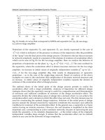
= 20 rad/s. Fig.4 shows the
desired trajectories in z and ψ.
One can observe that

γ
→ −124.6 rad/s remains bounded away from zero during the flight.
For the chosen trajectories and gains

γ
converges rapidly to a constant value (see Fig.7).
This is an interesting point to note since it shows that the dynamics and feedback control
yield flight conditions close to the ones of real helicopters which fly with a constant

γ
thanks to a local regulation feedback of the main rotor speed (which does not exist on the
VARIO scale model helicopter). One can also notice that the main rotor angular speed is
similar for the three controls as illustrated in Fig.7. The difference between the three controls
appears in Fig.6 where the tracking errors in z are less significant by using the (BACK) and
(ADRC) control than (RNFC) control. For ψ it is the different. This is explained by the use of
a PID controller for the (RNFC) and (ADRC) but a PD controller for the (BACK) controller of
ψ (Fig.6). Here, the (ADRC) and (BACK) controls show a robust behavior in presence of
noise.

Fig. 6. Tracking error in z and in ψ. Fig. 7. Variations of the main rotor thrust T
M

and the main rotor angular speed

γ .
Robust and Active Trajectory Tracking for an Autonomous Helicopter under Wind Gust

99
One can see in Fig.7 that the main rotor thrust converges to values that compensate the
helicopter weight, the drag force and the effect of the disturbance on the helicopter. The
(RNFC) control allows the main rotor thrust T
M
to be less away from its balance position
than the other controls, where the RNFC control is less sensitive to noise. Fig.9 represent the
effectiveness of the observer:
ˆ
x
3
and f
z
(y,
y

,w) are very close and also
ˆ
x
6
and f

ψ
(y,
y

,w).
Observer errors are presented in the Fig.8.


Fig. 8. Observer error in z and in ψ Fig. 9. Estimation of f
z
and of f
$

If one keeps the same parameters of adjustment for the three controls and using a larger
wind gust (v
raf
= 3m/s), we find that the control (BACK) give better results than the two
controls (ADRC) and (RNFC) (see Fig.10).


Fig. 10. Large disturbance v
raf
= 3m/s
Fig.11 shows the tracking error in z and ψ for two different ADRC controls. These errors are
quite simular for approach 1 (ADRC) and approach 2 (ADRCM). Nevertheless ADRCM
induces larger error at the take off, which can be explained by the fact that the control
depends directly on the angular velocity of the main rotor: this last one need a few time to
reach its equilibrium position as seen in Fig.6. The same argument can be invoked to explain
the saturation of ADRCM control u
1

and u
2
as illustrated in Fig.12.
Robotics, Automation and Control

100

Fig. 11. Tracking error in z and ψ for both Fig. 12. Inputs u
1
and u
2
for both approachs
approachs 1 and 2 of ADRC control. 1 and 2 of ADRC control.
7. Conclusion
In this chapter, a robust nonlinear feedback control (RNFC), an active disturbance rejection
control based on a nonlinear extended state observer (ADRC) and backstepping control
(BACK) have been applied for the drone helicopter control disturbed by a wind gust. The
technique of a robust nonlinear feedback control use the second method of Lyapunov and
an additional feedback provides an extra term Δv to overcome the effects of the uncertainty
and disturbances. The basis of ADRC is the extended state observer. The state estimation
and compensation of the change of helicopter parameters and disturbance variations are
implemented by ESO and NESO. By using ESO, the complete decoupling of the helicopter is
obtained. The major advantage of the proposed method is that the closed loop
characteristics of the helicopter system do not depend on the exact mathematical model of
the system.
The backstepping technique should not viewed as a rigid design procedure, but rather as a
design philosophy which can be bent and twisted to accommodate the specific needs of the
system at hand. In the particular example of an autonomous helicopter, we were able to
exploit the flexibility of backstepping with respect to the selection of virtual controls, initial
stabilizing functions and Lyapunov functions. Comparisons were made in detail between

the three methods of control.
It is concluded that the three proposed controls algorithms produces satisfactory dynamic
performances. Even for large disturbance, the proposed backstepping (BACK) and (ADRC)
control systems are robust against the modeling uncertainties and external disturbance in
various operating conditions. It is also indicated that (BACK) and (ADRC) achieve a better
tracking and stabilization with prescribed performance requirements.
For practical reasons, the second ADRC approach is the best one because it only requires to
know some aerodynamic parameters of the helicopter (dimensions of the blades of the main
and tail rotor and the helicopter weight), whereas the other approaches (first ADRC
Robust and Active Trajectory Tracking for an Autonomous Helicopter under Wind Gust

101
approach, RNCF and BACK) depend on all the aerodynamic parameters which generate the
forces and the couples that act on the helicopter. For first ADRC control, a stability analysis
has been carried out where boundness of states of helicopter and observer are proved in
spite of the presence of wind gust.
As illustrated in tables 2 and 3, wind gust induces large variation of helicopter parameters,
and the controls quoted in this work can efficiently treat these parameter deviations.
As perspective, this work is carried on a model of a 7DOF VARIO helicopter, where ADRC
and linearizing control will be tested in simulation. The first results using ADRC control on
this 7DOF helicopter have been recently obtained (see (Martini et al., 2008) ). Moreover, our
control methodologies will be also implemented on a new platform to be built using a Tiny
CP3 helicopter.
8. References
Beji, L. and A. Abichou (2005). Trajectory generation and tracking of a minirotorcraft.
Proceedings of the 2005 IEEE International Conference on Robotics and Automation,
Spain, 2618–2623.
Benaskeur, A., L. Paquin, and A. Desbiens (2000). Toward industrial control applications of
the backstepping. Process Control and Instrumentation, 62–67.
Dzul, A., R. Lozano, and P. Castillo (2004). Adaptive control for a radio-controlled helicopter

in a vertical flying stand. International journal of adaptive control and signal processing
18, 473–485.
Frazzoli, E., M. Dahleh, and E. Feron (2000). Trajectory tracking control design for
autonomous helicopters using a backstepping algorithm. Proceedings of the American
Control Conference Chicago, Illinois, 4102–4107.
Gao, Z., S. Hu, and F. Jiang (2001). A novel motion control design approach based on active
disturbance rejection. pp. 4877–4882. Orlando, Florida USA: Proceedings of the 40th
IEEE Conference on Decision and Control.
G.D.Padfield (1996). Helicopter Flight Dynamics: The Theory and Application of Flying
Qualities and Simulation Modeling. Blackwell Science LTD.
Han, J. (1999). Nonlinear design methods for control systems. Beijing, China: The Proc of the
14th IFAC World Congress.
Hauser, J., S. Sastry, and G. Meyer (1992). Nonlinear control design for slightly non-
minimum phase systems: Applications to v/stol aircraft. Automatica 28 (4), 665–679.
Hou, Y., F. J. Z. Gao, and B. Boulter (2001). Active disturbance rejection control for web
tension regulation. Proceedings of the 40th IEEE Conference on Decision and Control,
Orlando, Florida USA, 4974–4979.
Ifassiouen, H., M. Guisser, and H. Medromi (2007). Robust nonlinear control of a miniature
autonomous helicopter using sliding mode control structure. International Journal Of
Applied Mathematics and Computer Sciences 4 (1), 31–36.
Koo, T. and S. Sastry (1998). Output tracking control design of a helicopter model based on
approximate linearization. The 37th Conference on Decision and Control (Florida, USA)
4, 3636–3640.
Mahony, R. and T. Hamel (2004). Robust trajectory tracking for a scale model autonomous
helicopter. Int. J. Robust Nonlinear Control 14, 1035–1059.
Robotics, Automation and Control

102
Martini, A., F. Léonard, and G. Abba (2005). Suivi de trajectoire d’un hélicoptère drone sous
rafale de vent[in french]. CFM 17ème Congrès Français de Mécanique. Troyes, France,

CD ROM.N
0
.467.
Martini, A., F. Léonard, and G. Abba (2007a). Robust and active trajectory tracking for an
autonomous helicopter under wind gust. ICINCO International Conference on
Informatics in Control, Automation and Robotics, Angers, France 2, 333–340.
Martini, A., F. Léonard, and G. Abba (2007b). Suivi robuste de trajectoires d’un hélicoptère
drone sous rafale de vent. Revue SEE e-STA 4, 50–55.
Martini, A., F. Léonard, and G. Abba (2008, 22 -26 Septembre). Robust nonlinear control and
stability analysis of a 7dof model-scale helicopter under wind gust. In IEEE/RSJ,
IROS, International Conference of Intelligent Robots and Systems, to appear. NICE,
France.
McLean, D. and H. Matsuda (1998). Helicopter station-keeping: comparing LQR, fuzzy-logic
and neural-net controllers. Engineering Application of Artificial Intelligence 11, 411–
418.
Pflimlin, J., P. Soures, and T. Hamel (2004). Hovering flight stabilization in wind gusts for
ducted fan uav. Proc. 43 rd IEEE Conference on Decision and Control CDC, Atlantis,
Paradise Island, The Bahamas 4, 3491– 3496.
Sanders, C., P. DeBitetto, E. Feron, H. Vuong, and N. Leveson (1998). Hierarchical control of
small autonomous helicopters. 37th IEEE Conference on Decision and Control 4, 3629 –
3634.
Spong, M. and M. Vidyasagar (1989). Robot Dynamics and Control. John Willey and Sons.
Vilchis, A. (2001). Modélisation et Commande d’Hélicoptère. Ph. D. thesis, Institut National
Polytechnique de Grenoble.
Vilchis, A., B. Brogliato, L. Dzul, and R. Lozano (2003). Nonlinear modeling and control of
helicopters. Automatica 39, 1583 –1596.
Wei, W. (2001). Approximate output regulation of a class of nonlinear systems. Journal of
Process Control 11, 69–80.
Zhao, J. and I. Kanellakopoulos (1998). Flexible backstepping design for tracking and
disturbance attenuation. International journal of robust and nonlinear control 8, 331–

348.
6
An Artificial Neural Network Based Learning
Method for Mobile Robot Localization
Matthew Conforth and Yan Meng
Department of Electrical and Computer Engineering
Stevens Institute of Technology
Hoboken, NJ 07030, USA
1. Introduction
One of the most used artificial neural networks (ANNs) models is the well-known Multi-
Layer Perceptron (MLP) [Haykin, 1998]. The training process of MLPs for pattern
classification problems consists of two tasks, the first one is the selection of an appropriate
architecture for the problem, and the second is the adjustment of the connection weights of
the network.
Extensive research work has been conducted to attack this issue. Global search techniques,
with the ability to broaden the search space in the attempt to avoid local minima, has been
used for connection weights adjustment or architecture optimization of MLPs, such as
evolutionary algorithms (EA) [Eiben & Smith, 2003], simulated annealing (SA) [Jurjoatrucj et
al., 1983], tabu search (TS) [Glover, 1986], ant colony optimization (ACO) [Dorigo et al.,
1996] and particle swarm optimization (PSO) [Kennedy & Eberhart, 1995]. The
NeuroEvolution of Augmenting Topologies (NEAT) [Stanley & Miikkulainen, 2002] method
turns the neural networks topology and connect weight simultaneioulsy using an
evolutionary computation method. It evolves efficient ANN solutions quickly by
complexifying and optimizing simultaneously; it achieves performance that is superior to
comparable fixed-topology methods. In [Patan & Parisini, 2002] the stochastic methods
Adaptive Random Search (ARS) and Simultaneous Perturbation Stochastic Approximation
(SPSA) outperformed extended dynamic backpropagation at training a dynamic neural
network to control a sugar factory actuator. Recently, artifical neural networks based
methods are applied to robotic systems. In [Racz & Dubrawski, 1994], an ANN was trained
to estimate a robot’s position relative to a particular local object. Robot localization was

achieved by using entropy nets to implement a regression tree as an ANN in [Sethi & Yu,
1990]. An ANN was trained in [Choi & Oh, 2007] to correct the pose estimates from
odometry using ultrasonic sensors.
In this paper, we propose an aritifucal neural networks learning method for mobile robot
localization, which combines the two popular swarm inspired methods in computational
intelligence areas: Ant Colony Optimization (ACO) and Particle Swarm Optimization (PSO)
to train the ANN models. ACO was inspired by the behaviors of ants and has many
successful applications in discrete optimization problems. The particle swarm concept
originated as a simulation of a simplified social system. It was found that the particle swarm
model could be used as an optimizer. These algorithms have been applied already to solving
Robotics, Automation and Control

104
problems of clustering, data mining, dynamic task allocation, and optimization [Lhotska et
al., 2006].
The basic idea of the proposed SWarm Intelligence-based Reinforcement Learning (SWIRL)
method is that ACO is used to optimize the topology structure of the ANN models, while
the PSO is used to adjust the connection weights of the ANN models based on the
optimized topology structure. This is designed to split the problem such that ACO and PSO
can both operate in the environment they are most suited for. ACO is ideally applied to
finding paths through graphs. One can treat the ANN’s neurons as vertices and its
connections as directed edges, thereby transforming the topology design into a graph
problem. PSO is best used to find the global maximum or minimum in a real-valued search
space. Considering each connection plus one associated fitness score as orthogonal
dimensions in a hyperspace, each possible weight configuration is merely a point in that
hyperspace. Finding the optimal weights is thus reduced to finding the global maximum of
the fitness function in that hyperspace.
The chapter is organized as follows. Section 2 introduces two swarm intelligence based
methods: ant colony optimiztion and particle swarm optimization. The proposed SWIRL
method is described in Section 3. Simulation results and discussions using SWIRL method

for mobile robot localization are presented in Section 4. Conclusions are given in Section 5.
2. Swarm intelligence
2.1 Ant colony optimization
Dorigo et al. [11] proposed an Ant Colony Optimization (ACO). ACO is essentially a system
that simulates the natural behavior of ants, including mechanisms of cooperation and
adaptation. The involved agents are steered toward local and global optimization through a
mechanism of feedback of simulated pheromones and pheromone intensity processing. It is
based on the following ideas. First, each path followed by an ant is associated with a
candidate solution for a given problem. Second, when an ant follows a path, the amount of
pheromone deposit on that path is proportional to the quality of the corresponding
candidate solution for the target problem. Third, when an ant has to choose between two or
more paths, the path(s) with a larger amount of pheromone are more attractive to the ant.
After some iterations, eventually, the ants will converge to a short path, which is expected to
be the optimum or a near-optimum solution for the target problem.
2.2 Particle swarm optimization
The PSO algorithm is a population-based optimization method, where a set of potential
solutions evolves to approach a convenient solution (or set of solutions) for a problem. The
social metaphor that led to this algorithm can be summarized as follows: the individuals
that are part of a society hold an opinion that is part of a "belief space" (the search space)
shared by every possible individual. Individuals may modify this "opinion state" based on
three factors: (1) The knowledge of the environment (explorative factor); (2) The individual's
previous history of states (cognitive factor); (3) The previous history of states of the
individual's neighborhood (social factor).
Therefore, the basic idea is to propel towards a probabilistic median, where explorative factor,
cognitive factor (local robot respective views), and social factor (global swarm wide views) are
considered simultaneously and try to merge these three factors into consistent behaviors for
each robot. The exploration factor can be easily emulated by random movement.
An Artificial Neural Network Based Learning Method for Mobile Robot Localization

105

3. The SWIRL approach
In the SWIRL approach, the ACO algorithm is utilized to select the topology of the neural
network, while the PSO algorithm is utilized to optimize the weights of the neural network.
The SWIRL approach is modeled on a school, with the ACO, PSO, and neural networks
taking on the roles of administrator, teacher, and student respectively. Students learn,
teachers train students, and administrators allocate resources to teachers. In the same
fashion, the ACO algorithm allocates training iterations to the PSO algorithms. The PSO
algorithms then run for their allotted iterations to train their neural networks. The global
best score for all the neural networks trained by a particular PSO instance is then used by
the ACO algorithm to reallocate the training iterations.
3.1 ACO-based topology optimization
ACO is used to allocate training iterations among a set of candidate network topologies.
The desirability in ACO is defined as:

1
1
)(
+
=
h
id
(1)
where h is the number of hidden nodes in neural network i.
τ
(pheromone concentration) is
initialized to 0.1, so that the ants' initial actions are based primarily on desirability.
τ
is then
updated according to:

sum
a
g
ig
intiti
)(
)(),()1,( ⋅+⋅=+
τρτ
(2)
where
ρ
is the rate of evaporation,
a
n is the number of ants returning from neural network
i, g(i) is the global best for i, and
s
um
g
is the sum of all the current global bests.
Each ant represents one training iteration for the PSO teacher. During each major iteration
(i.e. ACO step), the ants go out into the topology space. The probability ant k goes to neural
network i is given by:

{}
1
[(,)][ ()]
()
[(,)] [()]
i
j

it di
pi
jt d j
αβ
αβ
τ
τ
=
=
⋅
∑
(3)
where
α
and
β
are constant factors that control the relative influence of pheromones and
desirability, respectively.
3.2 PSO-based weight adjustment
The ANNs are then trained via the PSO algorithm for a number of iterations determined by
the number of ants at that node. Each PSO teacher starts with a group of networks whose
connection weights are randomly initialized. The student ANNs are tested on the chosen
problem and each receives a score. The PSO teacher keeps track of the global best
configuration and each student’s individual best configuration. A configuration for an ANN
with n connections can be considered as a point in an n+1 dimensional space, where the
extra dimension is for the reinforcement score. After every round of testing, the teacher
updates the connection weights of the student ANNs according to the following equations: