Robotics Automation and Control 2011 Part 6 doc

Environment Modelling with an Autonomous Mobile Robot for Cultural Heritage
Preservation and Remote Access

141
Advanced Mobile Robots, pp. 61–67, Kaiserlautern, Germany, ISBN 0-8186-7695-7,
October 1996, IEEE Computer Society, Los Alamitos
Gutmann, J. S. & Konolige, K. (1999), Incremental mapping of large cyclic environments,
Proceedings of IEEE International Symposium on Computational Intelligence in Robotics
and Automation, pp. 318-325 , Monterey, CA, ISBN 0-7803-5806-6, November 1999,
IEEE Computer Society, Los Alamitos
Hartley, R., (1997), Kruppa’s equations derived from the fundamental matrix, IEEE
Transactions on pattern analysis and machine intelligence, Vol. 19, No. 2, (February
1997), (133-135), ISSN 0162-8828
Hartley, R. & Zisserman, A. (2003). Multiple View Geometry in Computer Vision, 2nd edition,
Cambridge University Press, ISBN 0521540518
Hirzinger, G., Bodenmüller, T., Hirschmüller, H., Liu, R., Sepp, W., Suppa, M., Abmayr, T. &
Strackenbrock, B. (2005), Photo-realistic 3D modelling - From robotics perception
towards cultural heritage. Proceedings of International Workshop on Recording,
Modeling and Visualization of Cultural Heritage, Ascona, Switzerland, May 2005
Hough, P. V. C, (1962), Method and means for recognizing complex patterns, U.S. Patent
3069654
Ip Y. L. & Rad A. B. (2004), Incorporation of feature tracking into Simultaneous Localization
and Mapping building via sonar data, Journal of Intelligent and Robotic Systems, Vol.
39, No. 2, (February 2004), (149-172), ISSN 0921-0296
Kleinehagenbrock, M.; Lang S., Fritsch J., Lomker F., Fink G. & Sagerer G. (2002), Person
tracking with a mobile robot based on multi-modal anchoring, Proceedings of IEEE
Int. Workshop on Robot and Human Interactive Communication, pp. 423-429, ISBN 0-
7803-7545-9, Berlin, Germany, September 2002, IEEE Computer Society, Los
Alamitos
Leiva, J. M.; Martinez, P., Perez, E. J., Urdiales, C. & Sandoval, F. (2001), 3D Reconstruction
of static indoor environment by fusion of sonar and video data, Proceedings of Int.

Symposium on Intelligent Robotics Systems, pp.179-188, ISBN 2-907801-01-5, Toulouse,
France, July 2001, LAAS-CNRS, Toulouse
Lu, F. & Milios, E. (1997), Robot pose estimation in unknown environments by matching 2D
range scans, Journal of Intelligent and Robotic Systems, Vol. 18, No. 3, (March 1997),
(249–275), ISSN 0921-0296
Milella, A., Dimiccoli, C., Cicirelli, G. & Distante, A. (2007), A., Laser-based people-following
for human-augmented mapping of indoor environments, Proceedings of the 25th
IASTED International Multi-Conference: artificial intelligence and applications, pp. 151-
155, ISBN 978-0-88986-631-7, Innsbruck, Austria, February 12-14, 2007, ACTA Press
Anaheim, CA, USA
Nevado, M. M; Garcia-Bermejo, J. G., Casanova, E. Z. (2004), Obtaining 3D models of indoor
environments with a mobile robot by estimating local surface directions, Robotics
and Autonomous Systems, Vol. 48, No. 2-3, (September 2004), (131–143), ISSN 0921-
8890
Pineau J.; Montemerlo, M., Pollack, M., Roy, N. & Thrun, S. (2003), Towards robotic
assistants in nursing homes: challenges and results, Robotics and Autonomous
Systems, Vol. 42, No. 3-4, (March 2003), (271-281), ISSN 0921-8890
Robotics, Automation and Control

142
Se, S., Lowe, D. G. & Little, J. (2002), Mobile robot localization and mapping with
uncertainty using scale-invariant visual landmarks, International Journal of Robotics
Research, Vol. 21, No. 8, (August 2002), (735-758), ISSN 0278-3649
Sequeira, V., Ng, K., Wolfart, E., Gonçalves, J. G. M., Hogg, D. C. (1999), Automated
Reconstruction of 3D Models from Real Environments, ISPRS Journal of
Photogrammetry and Remote Sensing, Vol. 54, No. 1, (February 1999), (1-22), ISSN
0924-2716
Stachniss, C; Hanhel, D., Burgard W. & Grisetti, G. (2005), On actively closing loops in grid-
based fast-slam, Advanced Robotics, Vol. 19, No. 10, (1059-1079), ISSN 0169-1864
Thrun, S.; Beetz, M. Bennewitz, M., Burgard, W., Cremers, A. B., Dellaert, F., Fox, D.,

Hahnel, D., Rosenberg, C., Roy, N., Schulte, J. & Schulz, D. (2000), Probabilistic
algorithms and the interactive museum tour-guide robot minerva, The International
Journal of Robotics Research, Vol. 19, No. 11, (November 2000), (972-999), ISSN 0278-
3649
Thrun, S; Liu, Y., Koller D., Ng, A. Y., Ghahramani, Z., Durrant-Whyte, H., (2004),
Simultaneous Mapping and Localization with Sparse Extended Information Filters:
Theory and Initial Results, International Journal of Robotics Research, Vol. 23, No. 7-8
(July-August 2004), (693-716), ISSN 0278-3649
Topp, E. A. & Christensen, H. I. (2005). Tracking for Following and Passing Persons,
Proceedings of IEEE/RSJ Int. Conference on Intelligent Robots and Systems (IROS), pp.
2321-2327, ISBN 0-7803-8913-1, Edmonton, Alberta, Canada, August 2005, IEEE
Computer Society, Los Alamitos
Trahanias, P.; Burgard, W., Argyros A., Hahnel, D., Baltzakis, H., Pfaff, P. & Stachniss, C.
(2005), TOURBOT and WebFAIR: Web-operated mobile robots for telepresence in
populated exhibitions, IEEE Robotics & Automation Magazine, Vol. 12, No. 2, (June
2005), (77-89), ISSN 1070-98932
Wolf, D.F. & Sukhatme, G. S. (2005), Mobile robot simultaneous localization and mapping in
dynamic environment”, Autonomous Robots, Vol. 19, No. 1, (July 2005), (53-65), ISSN
0929-5593
Zhang, Z., Deriche, R., Faugeras, O., Luong, Q. (1994), A robust technique for matching two
uncalibrated images trough the recovery of the unknown epipolar geometry,
Technical report N° 2273, Institut national de recherche en informatique et en
automatique.
9
On-line Cutting Tool Condition Monitoring in
Machining Processes using
Artificial Intelligence
Antonio J. Vallejo
1
, Rubén Morales-Menéndez

2
and J.R. Alique
3

1
Visiting scholar at the Instituto de Automática Industrial, Madrid, Spain
2
Tecnológico de Monterrey, Monterrey NL,
3
Instituto de Automática Industrial, Madrid,
1,3
Spain
2
México
1. Introduction
High Speed Machining (HSM) has become one of the leading methods in the improvement
of machining productivity. The term HSM covers high spindle speeds, high feed rates, as
well as high acceleration and deceleration rates. Furthermore, HSM does not imply only
working with high speeds but also with high levels of precision and accuracy.
Additional to the HSM, many companies producing machine tools are interested in new
technologies which provide intelligent features. Several research works (Koren et al., 1999;
Erol et al., 2000; Liang et al., 2004) predict that future manufacturing systems will have
intelligent functions to enhance their own processes, and the ability to perform an effective,
reliable, and superior manufacturing procedures. In the areas of process monitoring and
control, these new systems will also have a higher process technology level.
In any typical metal-cutting process, the key indexes which define the product quality are
dimensional accuracy and surface roughness; both directly influenced by the cutting tool
condition. One of the main goals in a Computer Numerically Controlled (CNC) machining
centre is to find an appropriate trade-off among cutting tool condition, surface quality and
productivity. A cutting tool condition monitoring system which optimizes the operating

cost with the same quality of the product would be widely appreciated, (Saglam & Unuvar,
2003; Haber & Alique, 2003). For example, in (Tönshoff et al., 1988), it has been
demonstrated that effective machining time of the CNC milling centre could be increased
from 10 to 65% with a monitoring and control system. Also, (Sick, 2002) mentions that any
manufacturing process can be significantly optimized using a reliable and flexible tool
monitoring system.
The system must develop the following tasks:
• Collisions detection as fast as possible.
• Tool fracture identification.
• Estimation or classification of tool wear caused by abrasion or other influences.
While collision and tool fracture are sudden and mostly unexpected events that require
reactions in real-time, the development of wear is a slow procedure. This section focuses on
Robotics, Automation and Control

144
the estimation of wear. The importance of tool wear monitoring is implied by exchanging
worn tools in time, and tool costs can be reduced with a precise exploitation of the tool's
lifetime.
However, cutting tool monitoring is not an easy task for several reasons. First, the
machining processes are non-linear, and time-variant systems, which makes them difficult
to model. Secondly, the acquired signals from sensors are dependent on other kind of
factors, such as machining conditions, cutting tool geometry, workpiece material, among
others. There is not a direct method for measuring the cutting tool wear, so indirect
measurements are needed for its estimation. Besides, signals coming from machine tools
sensors are disturbed by many other reasons such as cutting tool outbreaks, chatter, tool
geometry variances, workpiece material properties, digitizers noise, sensor nonlinearity,
among others. There is not a straightforward solution.

Symbol Description Symbol Description
A State transition probability distribution

MFCC
Mel Frequency Cepstrum Coeff.
AC Accelerometer
MR
Multiple Regression
AE
Acoustic Emission M Number of distinct obs. symbols
a
e
Radial depth of cut (mm) N Spindle speed (rpm)
a
ij
Elements of the transition matrix N
s
Number of states in the model
ANN
Artificial Neural Networks N
f
Number of bandpass filters
a
p
Axial depth of cut (mm) n
p
Number of passes over workpiece
BN
Bayesian Networks O Observation sequence of model
B Obs. symbol probability distribution q
t
State at time t
CNC

Computer Numerically Controlled S State sequence in the model
Curv Machining geometry curvature(mm
-1
)
SOFM
Self-Organizing Feature Maps
DY Dynamometer
SP
Spindle Power
DOE
Design Of Experiments T Length of observation sequence
D
tool
Diameter of the cutting tool (mm) T
c
Tool life (min)
FFT
Fast Fourier Transform T
mach
Machining time (min)
FAR
False Alarm Rate Tr Training dataset
FFR
False Fault Rate Ts Testing dataset
f
HZ
Sampling frequency (Hz) V Set of individual symbols
f
Mel
Scale Mel frequency VB

Flank wear (mm or μm)
f
z
Feed per tooth (mm/rev/tooth) VB1
Uniform flank wear (mm o μm)
Fx Cutting force in x-axis (N) VB2
Non-uniform wear (mm o μm)
Fy Cutting force in y-axis (N) VB3
Localized flank wear (mm o μm)
Fz Cutting force in z-axis (N) Vol Volume of removal metal (mm
3
)
HB Brinell Hardness Number of the
workpiece (BHN)
x Sample
HMM
Hidden Markov Models z Number of teeth of cutting tool
HSM
High Speed Machining
λ
HMM model specification
LVQ
Learning Vector Quantization
π
Initial state distribution for HMM
L Machining length (mm)
μ
Mean value
M Log bandpass filter output amplitude
σ

Standard deviation
Table 1. Nomenclature.
This work proposes new ideas for the cutting tool condition monitoring and diagnosis with
intelligent features (i.e. pattern recognition, learning, knowledge acquisition, and inference
from incomplete information). Two techniques will be applied using Artificial Neural
On-line Cutting Tool Condition Monitoring in Machining Processes using Artificial Intelligence

145
Networks and Hidden Markov Models. The proposal is implemented for peripheral milling
process in HSM. Table 1 presents all the symbols and variables used in this chapter.
2. State of the art
The cutting tool wear condition is an important factor in all metal cutting processes.
However, direct monitoring systems are not easily implemented because their need of
ingenious measuring methods. For this reason, indirect measurements are required for the
estimation of cutting tool wear. Different machine tools sensors signals are used for
monitoring and diagnosing the cutting tool wear condition.
There are important contributions for cutting tool monitoring systems based on Artificial
Neural Networks (ANN), Bayesian Network (BN), Multiple Regression (MR) approaches
and stochastic methods.
In (Owsley et al., 1997), the authors presented an approach for monitoring the cutting tool
condition. Feature extraction from vibrations during the drilling is generated by Self-
Organizing Feature Maps (SOFM). The signals processing implies a spectral feature
extraction to obtain the time-frequency representation. These features are the inputs of a
HMM classifier. The authors demonstrated that SOFM are an appropriated algorithm for
vibration signals feature extraction.
A methodology based on frequency domain is presented by (Chen & Chen, 1999) for on-line
detection of cutting tool failure. At low frequencies, the frequency domain presents two
important peaks, which are compared to compute a ratio that could be an indicator for
monitoring tool breakage.
In (Atlas et al., 2000), the authors used HMM for the evaluation of tool wear in milling

processes. The feature extraction from vibrations signals were the root mean squared, the
energy and its derivative. Two cutting tool conditions were defined: worn and no-worn
condition. The reported success was around 93%.
In (Sick, 2002a), a new hybrid technique for cutting tool wear monitoring, which fuses a
physical process model with an ANN model is proposed for turning. The physical model
describes the influence of cutting conditions on measure force signals and it is used to
normalize them. The ANN model establishes a relationship between the normalized force
signals and the wear state of the cutting tool. The performance for the best model was 99.4%
for the learning step, and 70.0% for the testing step.
In (Haber & Alique, 2003) is developed an intelligent supervisory system for cutting tool
wear prediction using a model-based approach. The dynamic behavior of the cutting force
is associated with the cutting tool and process conditions. First, an ANN model is trained
considering the cutting force, the feed rate, and the radial depth of the cut. Secondly, the
residual error obtained from the measure and predicted force is compared with an adaptive
threshold in order to estimate the cutting tool condition. This condition is classified as new,
half-worn, or worn cutting tool.
In (Saglam & Unuvar, 2003), the authors worked with multilayered ANN for the monitoring
and diagnosis of the cutting tool condition and surface roughness. The obtained success
rates were of 77% for tool wear and 80% for surface roughness.
In (Dey & Stori, 2004), a monitoring and diagnosis approach based on a BN is presented.
This approach integrates multiple process metrics from sensor sources in sequential
machining operations to identify the causes of process variations. It provides a probabilistic
Robotics, Automation and Control

146
confidence level of the diagnosis. The BN was trained with a set of 16 experiments, and the
performance was evaluated with 18 new experiments. The BN diagnosed the correct state
with a 60% confidence level in 16 of 18 cases.
In (Haber et al., 2004) is introduced an investigation of cutting tool wear monitoring in a
HSM process based on the analysis of different signals signatures in time and frequency

domains. The authors used sensorial information from dynamometers, accelerometers, and
acoustic emission sensors to obtain the deviation of representative variables. The tests were
designed for different cutting speeds and feed rates to determine the effects of a new and
worn cutting tool. Data was transformed from time to frequency domain using the Fast
Fourier Transform (FFT) algorithm. They concluded that second harmonics of tooth path
excitation frequency in the vibration signal are the best indicator for cutting tool wear
monitoring.
A proposal to exploit speech recognition frameworks in monitoring systems of the cutting
tool wear condition is presented in (Vallejo et al., 2005). Also, (Vallejo et al., 2006) presented
a new approach for online monitoring the cutting tool wear condition in face milling. The
proposal is based on continuous HMM classifier, and the feature vectors were computed
from the vibration signals between the cutting tool and the workpiece. The feature vectors
consisted of the Mel Frequency Cepstrum Coefficients (MFCC). The success to recognize the
cutting tool condition was 99.86% and 84.55%, for the training and testing dataset,
respectively. Also, in (Vallejo et al., 2007) an indirect monitoring approach based on
vibration measurements during the face milling process is proposed. The authors compared
the performance of three different algorithms: HMM, ANN, and Learning Vector
Quantization (LVQ). The HMM was the best algorithm with 84.24% accuracy, followed by
the LVQ algorithm with 60.31% accuracy. Table 2 summarizes all works discussed in this
section.
3. Experimental set-up
This research work was focused on covering a domain in mold and die industry with
different aluminium alloys. In this industry, the peripheral milling process is of great
importance, its geometry can be defined as a simple straight line or even as a different
geometry path including concave and convex curvatures.
The experiments took place in a HSM centre HS-1000 Kondia, with 25 KW drive motor,
three axis, maximum spindle speed 24,000 rpm, and a Siemens open Sinumerik 840D
controller, as shown in Figure 1. During the experiment several HSS end mill cutting tools
(25° helix angle, and 2-flute) from Sandvik Coromant were selected for the end milling
process, and different workpiece materials (Aluminium with hardness from 70 to 157 HBN)

were used. These materials were selected because they have important applications in the
aeronautic and mold manufacturing industry. Also, several cutting tool diameters (from 8 to
20 mm) were employed.
3.1 Design of experiments
Currently, the most of the research experiments are related to surface roughness and flank
wear (VB). In machining processes they only consider a specific combination of cutting tool
and workpiece material. Therefore, several authors have pointed out the importance of
building databases with information of different materials and cutting tools that allow
On-line Cutting Tool Condition Monitoring in Machining Processes using Artificial Intelligence

147
computing models by considering a complete domain in the machining process. The DOE
was defined to consider the most important factors affecting the surface roughness during
the peripheral end milling process, see (Vallejo et al., 2007a). Therefore, its results are
relevant to compute a surface roughness model as well as and a model to predict the cutting
tool condition.

Process
Monitoring
States
Sensor
Signals
Recognition
methods
References
Drilling Tool wear AC HMM (Owsley et al., 1997)
End
Milling
Tool Breakage (Normal,
Broke)

AC FFT
(Chen & Chen, 1999)
End
Milling
Tool wear
(Worn-no worn)
AC HMM (Atlas et al., 2000)
Turning
Tool wear
(Wear value)
Process
parameters
ANN Sick, 2002
Turning
Tool wear
(New, half worn, worn)
Process
parameters
ANN
(Haber & Alique, 2003)
Face
Milling
Tool wear
(Flank wear)
DY ANN
(Saglam & Unuvar,
2003)
Face
Milling
Tool wear

(Low-high)
AE, SP BN
(Dey & Stori, 2004)
Milling
Tool wear
(New, worn)
AE, DY, AC FFT (Haber et al., 2004)
Face
Milling
Tool wear (New, half-new,
half-worn, worn)
AC HMM (Vallejo et al., 2006)
Face
Milling
Tool wear (New, half-new,
half-worn, worn)
AC
HMM, ANN,
LVQ
(Vallejo et al., 2007)
Table 2. Comparison of different research efforts for monitoring the cutting tool condition.
The recognition method is defined by considering the machining process, sensor signals,
and the classification method.
The factors and levels were defined via the application of a screening factorial design over
the most important factors affecting the surface roughness. These factors and levels were the
following: feed per tooth (f
z
), cutting tool diameter (D
tool
), radial depth of cut (a

e
), hardness
of the workpiece material (HB), and the machining geometry curvature (Curv). Table 3
shows the factors and levels defined for the experiments. Table 4 presents the selected
aluminium alloys with the different cutting tools used in the experiments. The dimensions
of the workpiece were 100x170x25 mm, and they were designed to allow the machining of
four replicates. The designed geometries are depicted in Figure 2a, and the cutting tools are
shown in Figure 2b.
The machining domain in HSM was characterized by using different aluminium alloys,
cutting tools and several geometries (concave, convex and straight path) in peripheral
milling process, and the DOE considered the following steps:
1. Run a set of experiments with the cutting tool in sharp condition. During the
experimentation the process variables were recorded.
2. Wear the cutting tool with the harder aluminium alloys until reaching a specific flank
wear in agreement with ISO-8688 Tool life testing in milling.
3. Run other set of experiments with a different cutting tool wear condition.
4. Repeat the steps 2 and 3 until the cutting tool reaches the tool-life criteria.
Robotics, Automation and Control

148

Fig. 1. Experimental Set-up. CNC machining centre HS-1000 Kondia (Right side), and the
workpiece fixed to the table after the machined process (left side).

Fig. 2. a) Aluminium workpieces and geometries. b) Cutting tools for the experimentation.
Levels
f
z

(mm/rev/tooth)

D
tool

(mm)
a
e

(mm)
HB
(BHN)
Curv
(mm
-1
)
-2 0.025 8 1 71 -0.05
-1 0.05 10 2 93 -0.025
0 0.075 12 3 110 0
1 0.1 16 4 136 0.025
2 0.13 20 5 157 0.05
Table 3. Factors and levels defined for the experimentation.
Workpiece material
Hardness (HB)
Cutting tools
Diameter (mm)
5083-H111 (71 HB)
6082-T6 (93 HB)
2024-T3 (110 HB)
7022-T6 (136 HB)
7075-T6 (157 HB)
R216.32-08025-AP12AH10F (8 mm)

R216.32-10025-AP14AH10F (10 mm)
R216.32-12025-AP16AH10F (12 mm)
R216.32-16025-AP20AH10F (16 mm)
R216.32-20025-AP20AH10F (20 mm)
Table 4. Aluminium alloys and specifications of the cutting tools used in the
experimentation.
On-line Cutting Tool Condition Monitoring in Machining Processes using Artificial Intelligence

149
3.2 Tool life evaluation
In practical workshop environment, the time at which a tool ceases to produce workpieces
of the desired size or surface quality usually determines the end of useful tool life. It is
essential to define tool life as the total cutting time to reach a specified value of tool-life
criterion. Here, it is necessary to identify and classify the cutting tool deterioration
phenomena, and where it occurs at the cutting edges. The main numerical values of tool
deterioration used to determine tool life are the quantity of testing material required and the
cost of testing. The following concepts are given to explain the deterioration phenomena in
the cutting tool:
• Tool wear. Change in shape of the cutting edge part of a tool from its original shape,
resulting from progressive loss of tool material during cutting.
• Brittle fracture (chipping). Cracks occurrence in the cutting part of a tool followed by the
loss of small fragments of tool material.
• Tool deterioration measure. Quantity used to express the magnitude of a certain aspect of
tool deterioration by a numerical value.
• Tool-life criterion. Predetermined value of a specified tool deterioration measure
indicating the occurrence of a specified phenomenon.
• Tool life (T
c
). Total cutting time of the cutting part required to reach a specified tool-life
criterion.

In Figure 3, terms related to the tool deterioration phenomena on end milling cutters are
shown. These terms include:
• Flank wear (VB): Loss of tool material from the tool flanks, resulting in the progressive
development of the flank wear land.
• Uniform flank wear (VB1): Wear land which is normally of constant width and extends
over the tool flanks of the active cutting edge.
• Non-uniform wear (VB2): Wear land which has an irregular width and the original flank
varies at each position of measurement.
• Localized flank wear (VB3): Exaggerated and localized form of flank wear which develops
at a specific part of the flank.
The tool-life criterion can be a predetermined numerical value for any type of tool
deterioration that can be measured. If there are different forms of deterioration, they should
be recorded so when any so when any of the deterioration phenomena limits has been
attained, we can say the end of the tool life has been the end of the tool life has been
reached.
Predetermined numerical values of specific types of tool wear are recommended:
• For a width of the flank wear land (VB) the following tool life end points are
recommended:
1. Uniform wear: 0.3 mm averaged over all teeth.
2. Localized wear: 0.5 mm maximum on any individual tooth.
• When chipping occurs, it is to be treated as localized wear using a VB3 value equal to
0.5 mm as a tool-life end point.
Finally, flank wear measurement is carried out parallel to the surface of the wear land and in
a perpendicular direction to the original cutting edge. Although the flank wear land on a
significant portion of the flank wear may be of uniform size, there will be variations in its
value at other portions of the flank, depending on the tool profile and edge chipping. Values
of flank wear measurements are related to the area or position along the cutting edges at
which the measurement is made.
Robotics, Automation and Control

150

Fig. 3. Different terms in the flank wear are depicted for an end milling cutter (Taken from
ISO 8088-2, 1989).
Therefore, it was necessary to define a methodology to wear the cutting tool, and to use the
total tool-life during the experimentation. The assessment of the flank wear was taken as
tool-life criterion. The applied methodology considers the following steps:
1. The new cutting tools are specified and the DOE with the four replicates is made.
2. The flank wear is assessed and registered at the end of the experimentation.
3. The cutting tools are worn by using several workpiece materials, and during the
process the flank wear was observed until specific flank wear is reached.
4. The DOE is repeated with the new cutting tools conditions.
5. The steps 2, 3 and 4 are repeated (two more times), and the flank wear is measured and
registered at the end of the process.
Figure 4 shows the evolution of the tool wear during the experimentation until the
maximum tool-life criterion is reached. The experiments were interrupted at regular
intervals for measurement of the flank wear (VB). The flank wear pattern along the cutting
edge is showed as uniform wear over the surface (see Figure 5). In all cases, the tool wear
data corresponds to localized wear.
Milling is an interrupted operation, where the cutting tool edge enters and exits the workpiece
several times. The machining time of the tool in minutes was computed by Equation (1):

Nzf
nL
T
z
p
mach
××
×

= (1)
The volume of removed material volume was computed by Equation (2):
LnaaVol
ppe
=
(2)
On-line Cutting Tool Condition Monitoring in Machining Processes using Artificial Intelligence

151

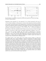
Fig. 4. Evolution of flank wear versus the volume of removal metal. The figure shows the
behavior of the five cutting tools.

Fig. 5. Evolution of flank wear on the cutting edge. The images were taken throught a
stereoscopic microscope. The cutting tool diameter is 12 mm.
The
VB was selected as the criterion to evaluate the tool’s life and its measurement was
carried out according to ISO 8688-2, 1989. These two variables,
Vol and VB, define the
evolution of the cutting tool wear. The range of the flank wear was selected so that four
cutting tool conditions were defined. They are shown in Table 5.

Cutting tool wear
condition
Flank wear
(mm)
New
0 ≤ VB < 0.08
Half-new
0.08 ≤ VB < 0.1

Half-worn
0.1 ≤ VB < 0.3
Worn
0.3 ≤ VB < 0.5
Table 5. Cutting tool wear conditions and the flank wear observed during the
experimentation.
Robotics, Automation and Control

152
3.3 Data acquisition system
The Data Acquisition System consists of several sensors that were installed in the CNC
machine (see Figure 6). For measuring the vibration, 2 PCB Piezotronics accelerometers
model 353B04 were fixed in x and y-axis directions on the workpiece. These instruments
have a sensitivity of 10 mV/g, in a frequency range from 0.35 to 20,000 Hz. Measurement
range is ±500g. Other 2 Bruel and Kjaer piezoelectric accelerometers model 4370, and
another model 4371, with a charge sensitivity of 98±2% pC/g, were installed on a ring fixed
to the spindle. Also, these sensors allow the recording of vibration in x, y, and z-axis, during
the cutting process.

Fig. 6. Experimental Set-up. CNC machining centre and data acquisition system (sensors,
amplifiers, boards and LabView interface). The vibration signals of the spindle and
workpiece, and forces during machining process were acquired with the NI-6152 board. The
acoustic emission signals were acquired with 1602 CompuScope board.
The dynamic cutting force components (Fx, Fy, Fz) were sensed with a 3 component force
dynamometer, on which the workpiece was mounted. All the signals were acquired with a
high speed multifunction DAQ NI-6152 card, which ensures 16-bit accuracy at a sampling
rate of 1.25 MS/s. The system was configured to obtain the signals with a sampling rate of
40,000 samples/s.
The acoustic emissions were recorded with 2 Kistler Piezotron
AE sensors model 8152B1,

with frequency range from 50 to 400 KHz, and sensitivity of 700 V/(m/s). One was installed
on a ring fixed to the spindle, and another was installed on the table of the machining
centre. The AE signals were acquired with a CompuScope 1602 card for PCI bus, with 16 bit
resolution. It provides a dual-channel simultaneous sampling rate of 2.5 MS/s. This board
was configured to obtain signals with a sampling rate of 1,000,000 samples/s. The
On-line Cutting Tool Condition Monitoring in Machining Processes using Artificial Intelligence

153
acquisition system was controlled with a LabView program. This program was used to
control the start and end of the recorded signal and storage the information in specific files.
4. Processing of the process variables
Signals from the sensors must be processed to obtain the relevant features which identify
the cutting tool condition. Basically, the raw signals undergo three steps in the signal
processing:
1.
Signal segmentation. During the machining process only one specific segment of the
signal was selected and processed. This signal segment was divided into 20 small
frames, which correspond to 0.15 (approximately) seconds of the machining time.
2.
Features extraction. The feature vectors were computed for all the frames of each signal.
3.
Average value. An average value was computed for all frames.
4.1 Feature extraction
The acquired signals during the machining process contain abundant information of the tool
status, such as, fundamental frequencies related with the spindle speed and number of
inserts, wide band frequency, amplitude of vibration signal, the sensitivity to detect the tool
condition, the chatter, and so forth. The different signals are pre-processed calculating their
MFCC representation, (Deller et al., 1993). This common transformation has shown to be
more robust and reliable than other techniques, (Davis & Mermelstaein, 1980). There is a
mapping between the real frequency scale (

HZ
f ) and the perceived frequency scale (
Mel
f ).
The Mel scale is defined by the following equation

⎟
⎠
⎞
⎜
⎝
⎛
+×=
700
f
1log2595f
Hz
Mel
(3)
The process to calculate the
MFCC is shown in Figure 7. In this process, we must define the
number of filters (N
f
), sampling frequency (f
HZ
), filters amplitude, and the configuration of
the filter banks (triangular or rectangular shape). At the end, the MFCC are computed using
the Inverse Discrete Cosine Transform:

∑

=
⎟
⎟
⎠
⎞
⎜
⎜
⎝
⎛
−=
N
1j
f
j
f
i
)5.0j(
N
i
cosm
N
2
MFCC
π
(4)
The result is a seven-dimension vector, where each dimensions correspond to one
parameter.
MFCC were computed by using the VOICEBOX: Speech Processing Toolbox for
MatLab, and written by (Brookes, 2006). The routines taken from Speech Recognition
module were: (a) The routine

melcepst, which implements a mel-cepstrum front end for a
recognizer; and (b) The routine
melbankm, which generates the associated bandpass filter
matrix.
4.2 MFCC for vibrations and force signals
Specifically for vibrations and force signals, the MFCC were computed by considering the
following parameters: number of filters 20, sampling rate 40,000 Hz, and a bandpass filter
with a triangular shape. The feature vector was of 7 dimensions (1 energy coefficient and 6
MFCC coefficients).
Robotics, Automation and Control

154

Fig. 7. Feature extraction process. The process variables (signals) are segmented and divided
in short frames. A Discrete Fourier Transform and a mapping between the real frequency
and the Mel frequency are computed. Then, a bandpass filters bank is applied for smoothing
the scaled spectrum. Finally, the
MFCC are computed using the discrete cosine transform.
4.3 MFCC for acoustic emission signals
MFCC were computed by considering the following parameters: number of filters 20,
sampling rate 1,000,000 Hz, and a triangular shape bandpass filter. The feature vector was of
7 dimensions (1 energy coefficient and 6 MFCC coefficients).
5. Monitoring and diagnose the cutting tool wear condition with HMM
Real world processes generally produce observable outputs which can be characterized as
signals. The signals can be discrete in nature (e.g., characters from a finite alphabet,
quantized vectors from a codebook, etc.), or continuous in nature (e.g., speech samples,
temperature measurements, vibration signals, music, etc.). They can be stationary or non-
stationary, pure or corrupted from other signal sources. A problem of fundamental interest
is characterizing such real-world signals in terms of signal models.
There are many reasons to consider this issue. First, a signal model can provide the basis for

the theoretical description of a signal processing system that can be used to process the
signal so as to provide a desired output. A second reason why signal models are important
is that they are potentially capable of letting us learn a great deal about the signal source.
But, the most important reason why signal models are significant is that they often work
On-line Cutting Tool Condition Monitoring in Machining Processes using Artificial Intelligence

155
extremely well in practice, and enable us to realize important practical systems (e.g.
prediction systems, recognition systems, identification systems, among others.).
Signal models can be divided into deterministic and statistical models. Deterministic models
generally exploit some known specific properties of the signal, and we only need to
determine the values of the signal model parameters (e.g., amplitude, frequency, phase,
etc.). On the other hand, statistical models use the statistical properties of the signal.
Examples of such statistical models include Gaussian, Poison, Markov, and Hidden Markov
processes. In this section, we are going to describe one type of stochastic signal model,
namely
HMM. A complete description of the HMM can be found in (Rabiner, 1989;
Mohamed & Gader, 2000).
5.1 Discrete Markov Processes
Consider a system which may be described at any time as being in one of a set of N
s
distinct
states, S
1
, S
2
, S
3
, , S
N

, as depicted in Figure 8 (where N
s
=3). At regularly spaced discrete
times, the system undergoes a change of state (possibly back to the same state) according to
a set of probabilities associated with the state.
The time instants associated with the state changes are t = 1, 2, , and the actual state at time
t, as q
t.
A full probabilistic description of the above system would, in general, require
specification of the current state (at time t), as well as all the predecessor states. For the
special case of a discrete, first order, Markov chain, this probabilistic description is reduced
to just the current and the predecessor state, as shown in the following equation,

]SqSq[P],Sq,SqSq[P
i1tjt
k
2ti1tjt
======
−−−
…
(5)
Furthermore we only consider those processes in which the right-hand side of (5) is
independent of time, thereby leading to the set of state transition probabilities a
i,j
of the form

Nj,i1],SqSq[Pa
i1tjtij
≤≤===
−

(6)


Fig. 8. Representation of a
HMM with three states and the probabilities of the transition
matrix (a
ij
).
with the state transition coefficients having the properties
Robotics, Automation and Control

156
a
ij
≥0

∑
=
=
N
1j
ij
1a (7)
Because, they obey standard stochastic constraints. The above stochastic process could be
called an observation Markov model since the output of the process is the set of states at
each instant of time, where each state corresponds to a physical event.
5.2 Extension to Hidden Markov Process
In this part we extend the concept of Markov models to include the case where the
observation is a probabilistic function of the state, and the resulting model (which is called a
HMM) is a doubly embedded stochastic process with an underlying stochastic process that

is not observable, but can only be observed through another set of stochastic processes that
produce the sequence of observations. To explain this concept, the following example is
presented.
Coin Toss Models. Assume that somebody is in a room behind the wall, and he can not see
what is happening inside. On the other side of the wall is another person who is performing
a coin tossing experiment. The other person will not tell you anything about what he is
exactly doing; he will only tell you the result of each coin flip. After a sequence of hidden
coin tossing experiments is performed, the observation sequence consisting of a series of
heads and tails, would be
O=O
1
O
2
O
3
O
T
(8)
=H H J J J H J J H H
where H stands for heads and J stand for tails. Given the above scenario, the problem of
interest is how do we build an
HMM to explain the observed sequence of heads and tails.
The first faced problem is deciding what states in the model correspond with what was
observed. Then we should decide how many states should be in the model. One possible
choice would be to assume that only a single biased coin was being tossed. In this case we
could model the situation with a two-state model where each state corresponds to a side of
the coin (i.e., heads or tails). This model is depicted in Figure 9a.
A second form of
HMM for explaining the observed sequence of coin toss outcomes is given
in Figure 9b. In this case there are 2 states in the model and each state corresponds to a

different, biased coin being tossed. Each state is defined by a probability distribution of
heads and tails. Transitions between states are characterized by a state transition matrix. The
physical mechanism which accounts for how state transition is selected could be itself a set
of independent coin tosses, or some other probabilistic event.
A third model of
HMM for explaining the observed sequence of coin toss outcomes is
defined very similarly to the
HMM in Figure 8. This model corresponds to using 3 biased
coins, and choosing among them a probabilistic event. Given the opportunity to choose
among the three models in Figures 8 and 9 for the explanation of the observed sequence of
heads and tails, a natural question would be which model matches the bets the actual
observations.
It should be clear that the simple 1-coin model of Figure 9a has only 1 unknown parameter,
the model of Figure 9b has four unknown parameters, and the model of Figure 8 has nine
On-line Cutting Tool Condition Monitoring in Machining Processes using Artificial Intelligence

157
unknown parameters. Thus, with the greater degrees of freedom, the larger HMMs would
seem to inherently be more capable of modeling a series of coin tossing experiments than it
would be equivalent smaller models.


Fig. 9. (a)
HMM with one coin and the two states. (b) HMM with two coins and each state
with two observations.
An
HMM is characterized by the following:
•
The number of states in the model, N
s

. Generally the states are interconnected in such as
way that any state can be reached from any other state. We denote the individual states
as S=S
1
,S
2
, ,S
N
, and the state at time t as q
t
.
•
The number of distinct observation symbols per state, M. The individual symbols such
as V = v
1
,v
2
, ,v
M
(i.e., the symbols in the last example were H (heads) and J (tails)).
•
The state transition probability distribution A = a
ij
, where

Nj,i1],SqSq[Pa
i1tjtij
≤≤===
−
(9)

•
The observation symbol probability distribution in state j, B = b
j
(k), where

Mk1 ,Nj1 ],Sqt at v[P)k(b
jt
k
j
≤≤≤≤== (10)
The initial state distribution π = π
i
where

Ni1],Sq[P
i1i
≤
≤
=
=
π
(11)
Given appropriate values for N
s
, M, A, B, and π, the HMM can be used as a generator of an
observation sequence
O = O
1
O
2

, ,O
T

It can be seen from the above discussion that a complete specification of an HMM requires
specification of two model parameters (N
s
, and M), observation symbols, and three
probability measures A, B, and π. For convenience, the compact notation is used,

),B,A(
πλ
=
(12)
to indicate the complete parameter set of the model.
Robotics, Automation and Control

158
5.3 Baum-Welch algorithm to train the model
The Baum-Welch algorithm, (Rabiner, 1989), is used to adjust the model parameters to
maximize the probability of the observation sequence given by the model. The observation
sequence used to compute
the model parameters is called a training sequence. The training
problem is crucial in the applications of the
HMMs, because it allows us to optimally adapt
model parameters to observed training data. The Baum-Welch algorithm is an iterative
process that uses the forward and backward probabilities to solve the problem. The goal is
to obtain a new model
),B,A(
πλ
=

to maximize the function,

[
]
)Q,O(Plog
)O(P
)Q,O(P
),(Q
Q
λ
λ
λ
λλ
∑
= (13)
First, a current model is defined as
),B,A(
πλ
= , and used to estimate a new model as
),B,A(
πλ
=
. The new model must present a better likelihood than the first model to
reproduce the observation sequence. Based on this procedure, if we iteratively use
λ
in
place of
λ
and repeat the calculus, then we can improve the probability of O being observed
from the model until some limiting point is reached.

The result of the recalculation procedure is called a maximum likelihood estimate of the
HMM. At the end, the new set of parameters (means, variance, and transitions) is obtained
for each
HMM.
5.4 Viterbi algorithm
In pattern recognition applications, it is useful to associate an optimal sequence of states to a
sequence of observations, given the parameters of the model. In pattern recognition, the
feature vector, representing the observations, is known, but the sequence of states that
defines the model is unknown. A "reasonable" optimality criterion consists of choosing the
state sequence (or path) that brings a maximum likelihood with respect to a given model
(i.e., best "explains" the observation). This sequence can be determined recursively via the
Viterbi algorithm. This algorithm identifies the single best state sequence, Q={q
1
q
2
q
T
}
for the given observation sequence O={O
1
O
2
O
T
}, and makes use of two variables:
•
The highest likelihood δ
t
(i) along a single path among all the paths ending in state i at
time t:

]OOO,iqqq[Pmax)i(
t21t21
qq,q
t
1t21
λδ
……
…
==
−
(14)
•
A variable ψ
t
(i) which allows to keep track of the "best path" ending in state j at time t.
Using these two variables, the algorithm implies the following steps:
1.
Initialization

0
Ni1 )O(b)i(
i
1ii1
=
≤≤=
ψ
πδ
(15)
2.

Recursion
stjij1t
Ni1
t
Nj1 ,Tt2 ),O(b ]a)i([max)j(
s
≤
≤
≤
≤
=
−
≤≤
δ
δ


sij1t
Ni1
t
Nj1 ,Tt2 ],a)i([max arg)j(
s
≤
≤
≤
≤
=
−
≤≤
δ

ψ
(16)
On-line Cutting Tool Condition Monitoring in Machining Processes using Artificial Intelligence

159
3. Termination:

[
]
[]
)i(max argq
)i(maxP
T
Ni1
T
T
Ni1
δ
δ
≤≤
∗
≤≤
∗
=
=
(17)
4.
Path (state sequence) backtracking:
1,,2T,1Tt ),q(q
1t1tt

…−−==
∗
++
∗
ψ
(18)
The Viterbi algorithm delivers the best states path, which corresponds to the observations
sequence. This algorithm also computes likelihood along the best path.
The HMM models were computed by using the Hidden Markov Model Toolbox for MatLab.
The routines were written by (Murphy, 2005).
6. Results
This section presents the results that were obtained by applying two different artificial
intelligence techniques for monitoring and diagnosing the cutting tool condition during the
peripheral end milling process in
HSM: (1) Artificial Neural Network, and (2) Hidden
Markov Models. In agreement with the experiments, a database was built with 441
experiments: 110 experiments used a new cutting tool, 112 a half-new cutting tool, 110 a
half-worn cutting tool, and 109 a worn cutting tool. A MonteCarlo simulation for the
training/testing steps was implemented due to the stochasticity of the approach. The results
correspond to the average of 10 runs, where every time a different training data set (
Tr) and
testing data set (
Ts) was generated (Figure 10).


Fig. 10. Procedure for computing the approach performance. A random simulation for
splitting the experimental dataset in training/testing sets was implemented due to the
stochastic nature of the approaches.
6.1 Artificial neural network
To compare our results with classical approaches, the cutting tool wear condition was

modeled with an
ANN model. The application of ANN to on-line process monitoring systems
has attracted great interest due to their learning capabilities, noise suppression, and parallel
computability. A complete recopilation of research works in on-line and indirect tool wear
monitoring with ANN are presented in (Sick, 2002).
ANN is often defined as a computing
Robotics, Automation and Control

160
system made up of a number of simple elements called neurons, which possesses information
by its dynamic state response to external inputs. The neurons are arranged in a series of layers.
Multi-layer feed-forward networks are the most common architecture. Furthermore, there are
several learning algorithms for training neural networks. Backpropagation has proven to be
successful in many industrial applications and it is easily implemented.
The proposed architecture implies 12 input neurons, one hidden layer with 12 neurons, and
1 output neuron. Figure 11 shows the
ANN model, where the input neurons represent the
following information: feed per tooth, tool diameter, radial depth of cut, workpiece material
hardness, curvature, and the
MFCC vector (7 dimensions).


Fig. 11. ANN model implemented for monitoring and diagnosis the on-line cutting tool
condition.
We used a feedforward
ANN model and “tanh” activation function. The trained algorithm
was classical backpropagation. For computing, input data (f
z
, D
tool

, a
e
, HB, Curv, and MFCC
vector) was normalized and output data was mapped to [-1, 1]. All the experimental dataset
was normalized to avoid numerical inestability. First, the dataset was normalized by
considering the mean value (μ), and standard deviation (σ) with the following equation,

x
x
)x(f =
−
=
σ
μ
(19)
A second normalized method was applied:
bipolar sigmoidal. This method was used because
the minimum and maximum values are unknown in real-time. The non-linear
transformation prevent most values from being compressed into essentially the same values,
and it also compress the large outlier values. The
bipolar sigmoidal was applied with the
following equation:

)x(
)x(
e1
e1
)x(f
−
−

+
−
=
(20)
With respect to the output neuron, the cutting tool condition, these values were mapped
between the normalized tool-wear and tool-wear condition (see Table 6). Finally, the dataset
was randomly divided into two sets, training (70%), and testing (30%) sets, in order to
measure their generalization capacity.
On-line Cutting Tool Condition Monitoring in Machining Processes using Artificial Intelligence

161
Normalized tool condition Cutting tool condition
From +0.66 to +1.00 New
From 0.0 to +0.66 Half-new
From -0.66 to 0.0 Half-worn
From -1.00 to -0.66 Worn
Table 6. Tool-wear from ANN model is mapped with the tool-wear Cutting.
The performance of the
ANN model was computed for ten different sets of data, which
were selected in random form. The training and testing processes were programmed by
using MatLab software. The obtained results correspond to 8 different ANN models, all of
them with the same architecture but different MFCC vector. The MFCC were computed for
each of the process signals (accelerometers, forces, and acoustic emission). Table 7 shows
the results computed with different process signals. The obtained performance corresponds
to an avarage value from the ten data sets.

Data Workpiece Spindle X Y AE AE
sets Acc-X Acc-Y Acc-X Acc-Y Force Force Spindle Workp.
Training 90.2% 94.5% 97.8% 98.7% 94.2% 97.6% 99.9% 99.2%
Testing 31.3% 33.8% 40.4% 47.2% 48.5% 48.0% 89.9% 69.7%

Table 7. Performance for the training and testing data sets of the ANN model. The first two
columns define the success of the accelerometers on the workpiece. The next two, the
accelerometers installed on the spindle. The last two columns correspond with the Acoustic
Emission sensors.
Table 7 shows that
ANN model with acoustic emission signal (AE-Spindle) represents the
best model for testing dataset, with a performance of 89.9% and Mean Squared Error (
MSE)
of 0.10075. Figure 12 plots the obtained results of the diagnosis system, when the
ANN
model was tested for the prediction of the cutting tool condition.


Fig. 12. Diagnosis the cutting tool condition with the ANN(12,12,1) model. The MFCC were
computed for the acoustic emission signal (AE-Spindle).
Robotics, Automation and Control

162

Fig. 13. Flow diagram for monitoring and diagnosis the cutting tool wear condition with
continuous HMM. The features from signals are separeted into 2 branches. The training
branch leads leads to
HMM, and the diagnose branch uses the new observations and HMMs
to recognize the cutting tool condition.
6.2 Hidden Markov Model
Figure 13 shows the flow diagram implemented for monitoring and diagnosing the cutting
tool wear condition on-line with the
HMM model. First, the signals are processed and
splited into two: training and testing branches. Second, the training branch produces the
HMM parameters by using the Baum-Welch algorithm. In this case, four models were

computed to represent the four cutting tool conditions. Third, the testing branch uses the
preprocessed signals and the HMM to compute the P(O/λ) using the Viterbi algorithm for
each model. The model with higher probability is selected as result.
The
HMM framework was evaluated for different states and Gaussians in order to find the
optimum performance results. Three different configurations were defined with seven
MFCC:
1.
HMM with 3 states and 2 Gaussians
2.
HMM with 4 states and 2 Gaussians
3. HMM with 4 States and 4 Gaussians.
Figure 14 shows how the performance increases by increasing the states and Gaussians in
the
HMM approach. Based on this result, the selected configuration was with 4 states and 2
Gaussians, where the average performance was 77.51% for testing dataset. The process
signal was the
AE installed over the table.
On-line Cutting Tool Condition Monitoring in Machining Processes using Artificial Intelligence

163
HMM(7,3,2)
HMM(7,4,2)
HMM(7,4,4)
Fresh
Half-new
Half-worn
Worn
0%
10%

20%
30%
40%
50%
60%
70%
80%
90%

Fig. 14. Perfomance of the HMM with different configuration. The HMM were computed
with different number of states (3, 4) and Gaussians (2,4).
Figure 15 shows the performance of the
HMMs with the different signals. The acoustic
emission signals present the best performance. For the AE-Spindle signal, the average
performance was 99.4% for training dataset, and 95.1% for testing dataset.

0%
10%
20%
30%
40%
50%
60%
70%
80%
90%
100%
Acx-wk Acy-wk Acx-Sp Acy-Sp AE-Sp AE-Table
Fresh Half-new Half-worn Worn

Fig. 15. Performance of the HMM for the different process signals. The results correspond to
the obtained success for the testing dataset.
A classical test in a diagnosis system is to identify two alarms due to a false classification of
cutting tool condition. These alarms are: False Alarm Rate (
FAR), and False Fault Rate (FFR).
Robotics, Automation and Control

164
FAR
condition represents a damage tool, but it is not true. FFR condition corresponds to a
good state of the tool, but it is really damaged. The
FAR condition is not a problem for
diagnosis, but it reduces the productivity. However, the
FFR condition might represent an
expensive problem when the rate is high, because the tool can break before it is replaced.
Figure 16 shows the misclassification percentage due to the
FFR condition. The classifier
with the lower percentage of the
FFR was the HMM using the acoustic emission sensor.
Once again, the AE-spindle does not produce any
FFR condition.
Acx-wk
Acy-w k
Acx-Sp
Acy-Sp
AE-Sp
AE-Table
Fresh
Half-new
Half-worn

Worn
0%
10%
20%
30%
40%
50%
60%
70%

Fig. 16. Misclassification percentage in FFR alarms, for the
HMM with different process
signals.
7. Conclusions
This chapter presented new ideas for monitoring and diagnosis of the cutting tool condition
with two different algorithms for pattern recognition:
HMM, and ANN. The monitoring and
diagnosis system was implemented for peripheral milling process in
HSM, where several
Aluminium alloys and cutting tools were used. The flank wear (VB) was selected as the
criterion to evaluate the tool’s life and four cutting tool conditions were defined to be
recognized: New, half new, half worn, and worn condition.
Several sensors were used to record important process variables; accelerometer,
dynamometer, and acoustic emission. Feature vectors, based on the Mel Frequency
Cepstrum Coefficients, were computed to characterize the process signals during the
machining processes. First, with the cutting parameters and
MFCC, the cutting tool
condition was modeled with an
ANN model. The feedfoward ANN model and
backpropagation algorithm were used to define the

ANN model. The proposed architecture
implies 12 input neurons and one output neuron (cutting condition). The best results were
obtained by using the signals from the Acoustic Emission installed on the machine spindle.
The success rate for the
ANN model was 89.9% for the testing dataset.
On-line Cutting Tool Condition Monitoring in Machining Processes using Artificial Intelligence

165
Second, the HMM approach was configured with four states and two Gaussians, and the
HMM models were computed with each one of the process signals. The best result was
obtained with the signals coming from
AE-Spindle. The performance was 95.08% for testing
dataset, and 0.0% in the
FFR condition. It is very important to mention, that HMM approach
only uses one sensor to classify the cutting tool condition, while the ANN approach uses
sensor fusion of five cutting parameters and one process variable to get the reported
performance.
8. References
Atlas, L., Ostendorf, M., and Bernard, G. D., (2000). Hidden Markov Models for Machining
Tool-Wear.
IEEE, pp. 3887-3890.
Brookes, M., (2006). VOICEBOX: Speech Processing Toolbox for MatLab
( Exhibition
Road, London SW7 2BT, UK.
Chen, J.C., and Chen, W. (1999). A Tool Breakage Detection System using an Accelerometer
Sensor.
J. of Intelligent Manufacturing, 10(2), pp. 187-197.
Davis, B.S., and Mermelstaein P., (1980). Comparison of Parametric Representation for
Monosyllabic Word Recognition in Continuously Spoken Sentences.
IEEE

Transactions on Acoustic, Speech, and Signal Processing, 4(28), pp. 357-366.
Deller, J.R., Hansen, J.H., and Proakis, J.G., (1993). Discrete-Time Processing of Speech
Signals.
IEEE pres, NJ 08855-1331.
Dey, S., and Stori, J.A. (2004). A Bayesian Network Approach to Root Cause Diagnosis of
Process Variations.
International Journal of Machine Tools & Manufacture, (45), pp. 75-
91.
Erol, N.A., Altintas, Y., and Ito, M.R. (2000). Open System Architecture Modular Tool Kit for
Motion and Machining Process Control.
IEEE/ASME Transactions on Mechatronics,
5(3), pp. 281-291.
Haber, R.E. and Alique, A. (2003). Intelligent Process Supervision for Predicting Tool Wear
in Machining Processes.
Mechatronics, (13), pp. 825-849.
Haber, R.E., Jiménez, J.E., Peres, C.R., and Alique, J.R. (2004). An Investigation of Tool-Wear
Monitoring in a High-Speed Machining Process.
Sensors and Actuators A, (116), pp.
539-545.
ISO 8688-2, (1989). Tool Life Testing in Milling – Part 2: End Milling.
International Standard,
first edition.
Korem, Y., Heisel, U., Jovane, F., Moriwaki, T., Pritschow, G., Ulsoy, G. and Van Brussel, H.
(1999). Reconfigurable Manufacturing Systems.
Annals of the CIRP 48(2) , pp. 527-
540.
Liang, S.Y., Hecker, R.L., and Landers, R.G. (2004). Machining Process Monitoring and
Control: the State of the Art.
Manufacturing Science and Engineering, 126, pp. 297-310.
Mohamed, M.A., and Gader, P., (2000). Generalized Hidden Markov Models - Part I:

Theoretical Frameworks. IEEE Transactions on Fuzzy Systems, 8(1), pp. 67-81.
Murphy, K., (2005). Hidden Markov Model Toolbox for MatLab
(
Owsley, L.M., Atlas, L.E., and Bernard, G.D. (1997). Self-Organizing Feature Maps and
Hidden Markov Models for Machine-Tool Monitoring.
IEEE Transactions on Signals
Processing, 45(11), pp. 2787-2798.