New Developments in Robotics, Automation and Control 2009 Part 10 potx

Kohonen Feature Map Associative Memory with Refractoriness based on Area Representation

263
Layer, the output of the neuron i in the Map-Layer
map
i
x is calculated by


(
)
⎪
⎩
⎪
⎨
⎧
<
=
otherwise ,0
, if ,1
map
bi
map
i
d
x
θ
WX

(10)

where
map
b
θ
is the threshold of the neuron in the Map-Layer as follows:


(
)
minmaxmin
map
b
ddad −+=
θ
(11)

(
)
i
i
min
dd WX ,min
=

(12)

(
)
i
i

max
dd WX ,max
=

(13)

In Eq.(11),
()
5.00
<
< aa is the coefficient.
Then, the output of the neuron
k in the I/O-Layer
in
k
x is calculated as follows:


⎪
⎩
⎪
⎨
⎧
≥
=
otherwise ,0
if ,1
in
b
in

k
in
k
u
x
θ

(14)

∑
∑
=
=
1:
1
i
xi
ik
i
map
i
in
k
W
x
u

(15)

where

in
b
θ
is the threshold of the neuron in the I/O-Layer,
in
k
u is the internal state of the
neuron
k in the I/O-Layer.

2.3.2 Recall Process for Analog Patterns
In the recall process of the KFM-AR, when the analog pattern
X is given to the I/O-Layer,
the output of the neurons
i in the Map-Layer
map
i
x
is calculated by


(
)
⎩
⎨
⎧
<
=
otherwise ,0
, if ,1

ai
map
i
d
x
θ
WX

(16)

where
a
θ
is the threshold of the neuron in the Map-Layer.
Then, the output of the neuron k in the I/O-Layer
in
k
x is calculated as follows:

.
1
1:
∑
∑
=
=
i
xi
ik
i

map
i
in
k
W
x
x
(17)
New Developments in Robotics, Automation and Control

264
3. KFM Associative Memory with Refractoriness based on Area Represen-
tation

The conventional KFM associative memory (Ichiki et al., 1993) and KFMAM-AR (Abe &
Osana, 2006) cannot realize one-to-many associations.
In this paper, we propose the
Kohonen Feature Map Associative Memory with Refractoriness based on Area Represen-
tation (KFMAM-R-AR) which can realize one-to-many associations. The proposed model is
based on the KFMAM-AR, and the neurons in the Map-Layer have refractoriness. In the
proposed model, one-to-many associations are realized by the refractoriness of neurons.
On the other hand, although the conventional KFMAM-AR can realize associations for
analog patterns, it does not have enough robustness for damaged neurons. In this research,
the model which has enough robustness for damaged neurons when analog patterns are
memorized is realized by improvement of the calculation of the internal states of neurons in
the Map-Layer.

3.1 Learning Process
In the proposed model, the patterns are trained by the learning algorithm of the KFMAM-
AR described in 2.2.

3.2 Recall Process
In the recall process of the proposed model, when the pattern
X is given to the I/O-Layer,
the output of the neuron
i in the Map-Layer
map
i
x is calculated by


(
)
(
)
(
)
(
)
(
)
tufdHtx
map
i
recallmap
i
ir,=

(18)

()()
()
⎟
⎠
⎞
⎜
⎝
⎛
−
+
=
ε
Dd
dH
recall
ir
ir
,
exp1
1
,

(19)

where D is the constant which decides area size,
ε
is the steepness parameter.
()
ir,d is the
Euclid distance between the winner neuron

r
and the neuron i and is calculated by


(
)
.
argmax tur
map
i
i
=

(20)

Owing to
(
)()
ir,dH
recall
, the neurons which are far from the winner neuron become hard to
fire.
()
(
)
tuf
map
i
is calculated by

()
()
(
)
(
)
⎪
⎩
⎪
⎨
⎧
>>
=
otherwise ,0
and if ,1
minmap
i
mapmap
i
map
i
tutu
tuf
θθ

(21)


Kohonen Feature Map Associative Memory with Refractoriness based on Area Representation

265
where
()
tu
map
i
is the internal state of the neuron i in the Map-Layer at the time t ,
map
θ
and
min
θ
are the thresholds of the neuron in the Map-Layer.
map
θ
is calculated as follows:


(
)
minmaxmin
map
uuau −+=
θ
(22)
(
)
tuu
map
i

i
min
min=
(23)
(
)
tuu
map
i
i
max
max=
(24)

where
()
15.0 << aa is the coefficient.
In Eq.(18), when the binary pattern
X
is given to the I/O-Layer, the internal state of the
neuron
i in the Map-Layer at the time t ,
(
)
tu
map
i
is calculated by

()

(
)
()
∑
=
−−−=
t
d
map
i
d
r
in
i
in
map
i
dtxk
N
d
tu
0
,
1
α
WX

(25)

where

()
i
in
d WX , is the Euclid distance between the input pattern X and the connection
weights
i
W . In the recall process, since all neurons in the I/O-Layer not always receive the
input, the distance for the part where the pattern was given is calculated as follows:

() ( )
∑
∈
=
−=
Ck
k
ikki
in
WXd
1
2
,WX

(26)

where C shows the set of the neurons in the I/O-Layer which receive the input. In Eq.(25),
in
N
is the number of neurons which receive the input in the I/O-Layer,
α

is the scaling
factor of the refractoriness and
(
)
10
<
≤
rr
kk is the damping factor. The output of the neuron
k in the I/O-Layer at the time t ,
(
)
tx
in
k
is calculated by

()
(
)
⎪
⎩
⎪
⎨
⎧
≥
=
otherwise ,0
if ,1
in

b
in
k
in
k
tu
tx
θ

(27)
()
()
∑
∑
>
=
out
i
xi
ik
i
map
i
in
k
W
tx
tu
θ
:

1

(28)

where is the threshold of the neuron in the I/O-Layer, is the threshold for the
New Developments in Robotics, Automation and Control

266
output of the neuron in the Map-Layer.
On the other hand, when the analog pattern is given to the I/O-Layer at the time
t
,
()
tu
map
i

is calculated by

() () ()
∑∑
=
∈
=
−−−=
t
d
map
i
d

r
N
Ck
k
ikk
in
map
i
dtxkWXg
N
tu
in
0
1
.
1
α

(29)

Here,
()
⋅g is calculated as follows:

()
⎪
⎩
⎪
⎨
⎧

<
=
otherwise ,0
,1
b
b
bg
θ

(30)

where
b
θ
is the threshold.
In the conventional KFMAM-AR, the neurons whose Euclid distance between the input
vector and the connection weights are not over the threshold fire. In contrast, in the
proposed model, the neurons which have many elements whose difference between the
weight vector and the input vector are small can fire. The output of the neuron
k in the
I/O-Layer at the time
t ,
(
)
tx
in
k
is calculated as follows:

()

()
∑
∑
>
=
outmap
i
xi
ik
i
map
i
in
k
W
tx
tx
θ
:
.
1

(31)

4. Computer Experiment Results

In this section, we show the computer experiment results to demonstrate the effectiveness of
the proposed model. Table 1 shows the experimental conditions.

4.1 Association Result for Binary Patterns

Here, we show the association result of the proposed model for binary patterns. In this
experiment, the number of neurons in the I/O-Layer was set to 800(= 400
× 2) and the
number of neurons in the Map-Layer was set to 400. Figure 2 (a) shows an example of stored
binary pattern pairs.
Figure 3 shows the association result of the proposed model when “lion” was given. As
shown in this figure, the proposed model could realize one-to-many associations.

4.2 Association Result for Analog Patterns
Here, we show the association result of the proposed model for analog patterns. In this
experiment, the number of neurons in the I/O-Layer was set to 800(= 400
× 2) and the
number of neurons in the Map-Layer was set to 400. Figure 2 (b) shows an example of stored
analog pattern pairs.
Kohonen Feature Map Associative Memory with Refractoriness based on Area Representation

267
Figure 4 shows the association result of the proposed model when “lion” was given. As
shown in this figure, the proposed model could realize one-to-many associations for analog
patterns.

4.3 Storage Capacity
Here, we examined the storage capacity of the proposed model. In this experiment, we used
the proposed model which has 800(= 400
× 2) neurons in the I/O-Layer and 400/800 neurons
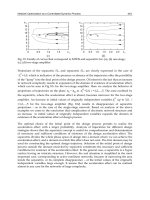
in the Map-Layer. We used random patterns and Figs.5 and 6 show the average of 100 trials.
In these figures, the horizontal axis is the number of stored pattern pairs, and the vertical
axis is the storage capacity. As shown in these figures, the storage capacity of the proposed
model for the training set including one-to-many relations is as large as that for the training
set including only one-to-one relations.

Parameters for learning
threshold(learning)
l
θ

7
10
−

initial value of
η

0
η

1.0
initial value of
σ

i
σ

0.3
last value of
σ

f
σ

5.0
steepness parameter
ε

01.0
coefficient (range of semi-fixed) D
0.3
Parameters for recall (common)
scaling factor of refractoriness
α

0.1
damping factor
r
k
9.0
steepness of
recall
H

ε

01.0
coefficient (size of area) D
0.3
threshold (minimum)
min
θ

5.0

threshold (output)
out
θ

99.0
Parameters for recall (binary)
coefficient (threshold) a
9.0
threshold in the I/O-Layer
in
b
θ
5.0
Parameter for recall (analog)
threshold (difference)
d
θ

1.0
Table 1. Experimental Conditions.
New Developments in Robotics, Automation and Control

268

(a) Binary Pattern (b) Analog Pattern
Fig. 2. An Example of Stored Patterns.


1=t 2
=

t 3
=
t 4
=
t 5
=
t
Fig. 3. Association Result for Binary Patterns.


1=t 2
=
t 3
=
t 4
=
t 5
=
t
Fig. 4. Association Result for Analog Patterns.

4.4 Recall Ability for One-to-Many Associations
Here, we examined the recall ability in one-to-many associations of the proposed model. In
Kohonen Feature Map Associative Memory with Refractoriness based on Area Representation

269
this experiment, we used the proposed model which has 800(= 400 × 2) neurons in the I/O-
Layer and 400 neurons in the Map-Layer. We used one-to-P(P = 1, 2, · · · , 30) random
patterns and Fig.7 shows the average of 100 trials. In Fig.7, the horizontal axis is the number
of stored pattern pairs, and the vertical axis is the recall rate. As shown in Fig.7, the

proposed model could recall all patterns when P is smaller than 15 (binary patterns) / 4
(analog patterns). Although the proposed model could not recall all patterns corresponding
to the input when P was 30, it could recall about 25 binary patterns / 17 analog patterns.

4.5 Noise Reduction Effect
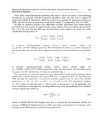
Here, we examined the noise reduction effect of the proposed model.
Figure 8 shows the noise sensitivity of the proposed model for analog patterns. In this
experiment, we used the proposed model which has 800(= 400 × 2) neurons in the I/O-Layer
and 400 neurons in the Map-Layer and 9 random analog patterns (three sets of patterns in
one-to-three relations) were stored. Figure 8 shows the average of 100 trials.
In the proposed model, the minimum threshold of the neurons in the Map-Layer
min
θ

influences the noise sensitivity. As shown in Fig.8, we confirmed that the proposed model is
more robust for noisy input when
min
θ
is small.


Fig. 5. Storage Capacity (400 neurons in the Map-Layer).
New Developments in Robotics, Automation and Control

270

Fig. 6. Storage Capacity (800 neurons in the Map-Layer).


Fig. 7. Recall Ability in One-to-Many Associations.

4.6 Robustness for Damaged Neurons
Here, we examined the robustness for damaged neurons of the proposed model.
Figure 9 shows the robustness for damaged neuron of the proposed model. In this
experiment, we used the proposed model which has 800(= 400
× 2) neurons in the I/OLayer
and 400 neurons in the Map-Layer and 9 random patterns (three sets of patterns in one-to-
three relations) were stored. In this experiment, n% of the neurons in the Map- Layer were
damaged randomly. Figure 9 shows the average of 100 trials. In this figure, the results of the
conventional KFMAM-AR were also shown.
From this result, we confirmed that the proposed model has the robustness for damaged
neurons.
Kohonen Feature Map Associative Memory with Refractoriness based on Area Representation

271
5. Conclusion

In this research, we have proposed the KFM Associative Memory with Refractoriness based
on Area Representation. The proposed model is based on the KFMAM-AR (Abe & Osana,
2006) and the neurons in the Map-Layer have refractoriness. We carried out a series of
computer experiments and confirmed that the proposed model has following features.
(1) It can realize one-to-many associations of binary patterns.
(2) It can realize one-to-many associations of analog patterns.
(3) It has robustness for noisy input.
(4) It has robustness for damaged neurons.


Fig. 8. Sensitivity to Noise (Analog Pattern).

Fig. 9. Robustness for Damaged Neurons.

New Developments in Robotics, Automation and Control

272
6. References

Abe, H. & Osana, Y. (2006). Kohonen feature map associative memory with area represen-
tation. Proceedings of IASTED Artificial Intelligence and Applications, Innsbruck.
Carpenter, G, A. & Grossberg, S. (1995). Pattern Recognition by Self-organizing Neural
Networks. The MIT Press.
Hattori, M. Arisumi, H. & Ito, H. (2002). SOM Associative Memory for Tempral Sequences.
Proceedings of IEEE and INNS International Joint Conference on Neural Networks, pp. 950-
955, Honolulu.
Hopfield, J. J. (1982). Neural networks and physical systems with emergent collective
computational abilities. Proceedings of National Academy Scienses USA, Vol.79,
pp.2554–2558.
Ichiki, H. Hagiwara, M. & Nakagawa, M. (1993). Kohonen feature maps as a supervised
learning machine. Proceedings of IEEE International Conference on Neural Networks,
pp.1944–1948.
Ikeda, N. & Hagiwara, M. (1997). A proposal of novel knowledge representation (Area
representation) and the implementation by neural network. International Conference on
Computational Intelligence and Neuroscience, III, pp. 430–433.
Kawasaki, N. Osana, Y. & Hagiwara, M. (2000) Chaotic associative memory for successive
learning using internal patterns. IEEE International Conference on Systems, Man and
Cybernetics.
Kohonen, T. (1994). Self-Organizing Maps, Springer.
Kosko, B. (1988). Bidirectional associative memories. IEEE Transactions on Neural Networks,
Vol.18, No.1, pp.49–60.
Osana, Y. & Hagiwara, M. (1999). Successive learning in chaotic neural network.
International Journal of Neural Systems, Vol.9, No.4, pp.285–299.
Rumelhart, D, E. McClelland, J, L. & the PDP Research Group. (1986). Parallel Distributed

Processing. Exploitations in the Microstructure of Cognition, Foundations, The MIT Press,
Vol.11.
Watanabe, M. Aihara, K. & Kondo, S. (1995). Automatic learning in chaotic neural networks.
IEICE-A, Vol.J78-A, No.6, pp.686–691.
Yamada, T. Hattori, M. Morisawa, M. & Ito, H. (1999). Sequential learning for associative
memory using Kohonen feature map. Proceedings of IEEE and INNS International Joint
Conference on Neural Networks, paper no.555, Washington D.C.
16

Incremental Motion Planning With Las Vegas
Algorithms

Jouandeau Nicolas, Touati Youcef and Ali Cherif Arab
University Paris8
France

1. Introduction

Las Vegas algorithm is a powerful paradigm for a class of decision problems that has at least
a theoretical exponential resolving time. Motion planning problems are one of those and are
out to be solved only by high computational systems due to such a complexity (Schwartz &
Sharir, 1983). As Las Vegas algorithms have a randomized way to meet problem solutions
(Latombe 1991), the complexity is reduced to polynomial runtime. In this chapter, we
present a new single shot random algorithm for motion planning problems. This algorithm
named RSRT for Rapidly-exploring Sorted Random Tree is based on inherent relation
analysis between Rapidly-exploring Random Tree components, named RRT components
(LaValle, 2004). RRT is an improvement of previous probabilistic motion planning
algorithms to address problems that involve wide configuration spaces. As the main goal of
the discipline is to develop practical and efficient solvers that automatically produce motion,
RRT methods successfully reduce the complexity in exploring the space partially and

producing non-deterministic solutions close to optimal ones. In the classical RRT algorithm,
space is explored by repeating successively three phases: generation of a random
configuration in the whole space (including free and non-free space); selection of a nearest
configuration; and generation of a new configuration obtained by numerical integration
over a fixed time step. Then the motion planning process is discretized into steps from the
initial configuration to other configurations in the space. In such a way, RRT algorithms are
the motion planners last generation that generally addresses a large set of motion planning
problems. Mobile, geometrical or functional constraints, input methods and collision
detection are unspecified. As it is possible to measure solutions provided by RRT, RSRT or
other improvements in spaces with arbitrary dimension, experiments are realized on a wide
set of path planning problems involving various mobiles in static and dynamic
environments. We experiment the RSRT and other RRT algorithms using various
configurations spaces to produce a massive experiment analysis: from free flying to
constraint mobiles, from single to articulated mobiles, from wide to narrow spaces, from
simple to complex distance metric evaluations, from special to randomly generated spaces.
These experiments show practical performances of each improvement, and results reflect
their classical behavior on each type of motion planning problems.

New Developments in Robotics, Automation and Control

274
2. RRT Sampling Based-planning

2.1 Principle
In its original formulation (LaValle, 1998), RRT method is described as a tree G = (V,E) ,
where V is the set of vertices and E the set of edges in the research space. From an initial
configuration q
init
, the objective is to generate a sequence of commands, leading a mobile M,
to explore all the configurations space C. The RRT method can solve this problem by

searching solution which spans a tree, where the configuration q
init
, describes the root node.
One can note that nodes and arcs represent respectively eligible configurations of M and
commands which are applied to move between the configurations. RRT method is a random
incremental search of configurations which permits a uniform exploration of the space. The
RRT implementation consists on a three phases: generate a configuration q
rand
, select a
configuration q
prox
inside the current tree, and integrate a new configuration q
new
from q
prox

towards q
rand
.
During the first phase, a random function is implemented to select an element of a
configurations space. The second phase consists of choosing q
prox
of G, which is the nearest
element of q
rand
. This phase is based on a metric
ρ
. Finally, a new configuration q
new
from

q
prox
towards q
rand
is generated and the objective is to implement a control which leads to
bring q
prox
closer to q
rand
. The new configuration q
new
is generated by integrating from q
prox
,
during a predefined time interval.

2.2 Graph construction of RRT method
Firstly, the RRT method is developed to solve planning problem in mobile robotic. In the
original algorithm, the possible constraints associated to M are not mentioned. During the
formulation of G, changes to be made for adding new constraints are minors, and the
precision depends mainly on the chosen local planning method. The graph elementary
construction in RRT method is described according to algorithm ALG. 1.

consRrt (q
init
, k , Δt , C )
init (q
init
, G )
for i in 1 to k

q
rand
= randConfig ( C )
q
prox
= nearestConfig (q
rand
, G )
q
new
= newConfig (q
prox
, q
rand ,
Δt )
addConfig (q
new
, G )
addEdge (q
prox
, q
new ,
G )
return G

nearestConfig (q
rand
, G )
d = inf
foreach q in G

if
ρ
( q , q
rand
) < d
q
prox
= q
d =
ρ
( q , q
rand
)
return q
prox

(1)
(2)

(3)
(4)







(5)

ALG. 1. Original RRT algorithm formulation
Incremental Motion Planning With Las Vegas Algorithms

275
We remark that the algorithm implements three functions. The first one, randConfig,
ensures a uniform partition of random samples in C, and guaranties uniform exploration
(Yershova & LaValle, 2004 and Lindemann et al., 2004). Function nearestConfig selects the
nearest configuration q
rand
of G. This relation proximity is defined by a distance metric
ρ
, as
it is illustrated in (ALG. 1. (5)). In the case of probabilistic methods PRM and RRT, the
nearest neighbour search with arbitrary dimension can be optimised (Yershova & LaValle,
2007 and Yershova & LaValle, 2002). Reducing of the search time of a nearest neighbour
permits to use a complex distance metric. A new configuration q
new
can be defined by
newConfig from q
prox
towards q
rand
. Knowing that M is subject to holonomic constraints, a
control inputs can be applied to move from q
prox
towards q
rand
with displacements

amplitudes Δt. Functions addConfig and addEdge add respectively q
new
to the list of nodes
of G and arcs between q
prox
and q
new
.

2.3 Cardinality and layer
For each new configuration q
new
in the generation phase, RRT method adds a configuration
by propagating q
prox
of G. In this case, no restriction on q
new
is imposed according to
configurations set G. So, q
new
can be similar to q
exist
, which can make possible to span a
graph with or without cycle. For example, let’s define Card as a cardinal of set, thus, if Card
( V ) = Card ( E ) + 1, then we can conclude that the graph is non-cyclic. To avoid stacking of
identical movements, each nodes q
prox
can’t be extended towards q
rand
for creating q

new
, if it
doesn’t already have a similar descendent.
If q
prox
is extended towards q
rand
, a new arc between q
prox
and q
new
is inserted in E.
If Card ( V ) ≤ Card ( E ), we can conclude that the graph contains at least one cycle. Thus, is
q
new
deleted and a new arc is inserted in E between q
prox
and q
exist
.
Creating cycles leads to decrease an expansion number of G in unexplored zones. However,
it permits to list possible solutions in the case of halt. Knowing that this scenario is more
topologic than geometric, RRT method is better without cycle [LAV98]. Fig 1 shows the
expansion of G respectively after 100, 500 and 1500 samples. Random samples have been
uniformly spread in the square. q
init
is initially in the center of the square. The mobile is a
simple point (without geometric shape) with holonomic constraints.

(a) (b) (c)
Fig. 1. Expansion of G in a free square (a after 100, b after 500 and c after 1500 samples)
New Developments in Robotics, Automation and Control

276
2.4 Natural expansion
The random distributions of samples which performs expansions, directs naturally the
growth of G towards the wider regions of space. This can be verified by constructing
Voronoï diagram which associates, for each new node of C, one Voronoï cell. For each
iteration of RRT method, the localization probability of the next random sample is more
important towards the largest cells of Voronoï diagram, which is defined by a previous
random samples set.
Let’s C
k
be a distribution of k random samples in the configurations space C. the
distribution C
k
converges in term of probability to C under condition of the uniformity of a
random samples partition in C (LaValle & Kuffner, 2000).
Knowing that Delaunay triangulation is a dual of Voronoï diagram, an example of a graph
expansion associated to RRT method is presented in Fig. 2. Graphs presented in (a), (b) and
(c) illustrate respectively the results of 25, 275 and 775 expansions including those of
Delaunay triangulations illustrated in (a’), (b’) and (c’). The space is two dimensional
squares without obstacles. For each iteration, adding a new item leads to construct a new
triangulation. In Fig. 2, initial configuration is represented by a circle in the center of the
space.

Fig. 2. Triangulation analysis due to samples
Incremental Motion Planning With Las Vegas Algorithms

277
The evolution of new configurations of G along iterations is illustrated in Fig 3. X-axis
represents the configuration number contained in the graph and Y-axis represents the
percentage of the entire surface S. The surface graph represents the average, minimal, and
maximal surface variations. In this case, the average surface is the average triangles surfaces.
The standard deviation graph represents the average, minimal and maximal standard
deviations. The initial configuration divides the space into four triangles with 0.25 in term of
surface and zero in standard deviation. The average area of triangles decreases linearly
according to the number of configurations.
In Figures 2, 3 and 4, positions in (a), (b) and (c) are placed around area average and
standard deviations curves. Maximum and minimum variations can increase or decrease
according to their relative positioning to the decreasing average value. Due to the
logarithmic scale, position of minimal variations vis-à-vis average values shows the almost-
equality between average value and minimum value. On the other hand, position of
maximal variations shows triangles much larger than the average value before a density
threshold (8.15 times larger before 353 configurations). From 353 configurations, the ratio
between the higher triangle and the average value progresses in stair-steps. Two stair-steps
p0 and p1 are placed on average and standard deviations curves as it’s illustrated in Fig 3.
This ratio tends to be stabilized around 2 from p1. The initial configuration position has no
influence on statistics relative to its expansion.


Fig. 3. Evolution of average, min and max of triangles areas during sampling
New Developments in Robotics, Automation and Control

278


Fig. 4. Evolution of standard deviation, min and max of deviation areas during sampling

2.5 End condition
A query of a mobile trajectory planning can be formulated according to a pair of
configuration-objective, which is instantiated on q
obj
or on a set of configurations C
obj
.
Restricting the search to a single configuration-objective can penalize the mobiles which are
subjected to dynamics or non-holonomics constraints. To improve the convergence towards
the objective, RRT resolutions implement a configuration q
obj
, whose components are not
fixed. Thus, the planning problem consists to find a path connecting q
init
to an element of
C
obj
. From q
init
, graph G seeks to achieve a configuration q
obj
. This can be done by a
successive adding of new configuration q
new

in the tree G. Variable k defines the number of
iterations required to solve the problem. In the case of k is not sufficient it is possible to
continue conducting research on new k iterations from the previously generated tree. The
construction of G is achieved when q
obj
∩ G=∅.

3. Related Works

In the previous section, C is presented without obstacle in an arbitrary space dimension. At
each iteration, a local planner is used to connect each couples ( q
new
, q
obj
) in C. The distance
between two configurations in T is defined by the time-step Δt. The local planner is
composed by temporal and geometrical integration constraints. The resulting solution
accuracy is mainly due to the chosen local planner. k defines the maximum depth of the
search. If no solution is found after k iterations, the search can be restarted with the previous
T without re-executing the init function. This principle can be enhanced with a bidirectional
search, shortened Bi-RRT (LaValle & Kuffner, 1999). Its principle is based on the
simultaneous construction of two trees (called T
init
and T
obj
that grows respectively from q
init

Incremental Motion Planning With Las Vegas Algorithms

279
and q
obj
. The two trees are developped towards each other while no connection is
established between them. This bidirectional search is justified because the meeting
configuration of the two trees is nearly the half-course of the initial configuration space.
Therefore, the resulting resolution time complexity is reduced (Russell & Norvig, 2003).
RRT-Connect is a variation of Bi-RRT that consequently increase the Bi-RRT convergence
towards a solution (Kuffner & LaValle, 2000) thanks to the enhancement of the two trees
convergence. This has been settled :
• to ensure a fast resolution for “simple” problems (in a space without obstacle, the
RRT growth should be faster (ALG.2. (1)) than in a space with many obstacles)
• to maintain the probabilistic convergence property. Using heuristics modify the
probability convergence towards the goal and also should modify its evolving
distribution. Modifying the random sampling can create local minima that could
slow down the algorithm convergence

connectRrt (q

, Δt , T )
r = ADVANCED
while r equals ADVANCED
r = expandT ( q
,
Δt , T )
return r


(1)

ALG. 2. Connecting a configuration q to T with RRT-Connect.

As it makes RRT less incremental, RRT-Connect is more adapted for non-differential
constraints (Cheng, 2001). It iteratively realize expansion by replacing a single iteration
(ALG. 1. (2)) with connectT function which corresponds to a succession of successful single
iterations (ALG. 2. (1)). An expansion towards a configuration q becomes either an extension
or a connection.

connectBiRrt (q
init
, q
obj
, k, Δt , C )
init ( q
init
, T
a
)
init ( q
obj
, T
b
)
for i in 1 to k
qrand = randConfig ( C )
r = expandRrt (q
rand
, Δt , T
a

)
if r not equals TRAPPED
if r equals REACHED
q
co
= q
rand

else
q
co
= q
new

if connectRrt (q
co
, T
a
, T
b
)
Return solution
swap (T
a
, T
b
)
return TRAPPED

ALG. 3. Expanding two graphs with RRTConnect

New Developments in Robotics, Automation and Control

280
According that two trees are constructed by Bi-RRT, growth is realized inside two trees
named T
a
and T
b
and a successfull connection of q
new
towards q
rand
in T
a
, implies many other
extensions (as many as the free space admits new free configurations, i.e. q
new
in C
free
) of
q
prox
found in T
b

towards q
new
. This new configuration q
new
becomes a convergence
configuration named q
co
(ALG. 3).
To improve the construction of T to an adequate progression of G in Cfree, previous works
propose :
• to deviate from its initial distribution the random sampling Bi-RRT and RRT-
Connect. Other Variations of RRT-Connect are called RRT-ExtCon, RRT-ConCon
and RRT-ExtExt; they modify the construction strategy of one of the two trees. The
priorities of extension and connection are balanced with new values according to
previous extensions (LaValle, 1998)
• to adapt q
prox
selection to a collision probability (Cheng & LaValle, 2001)
• to restrict q
prox
selection in an accessibility vicinity of the previous q
prox
in the
variation called RC-RRT (Cheng & LaValle, 2002)
• to bias sampling towards free spaces (Lindemann & LaValle, 2004)
• to parallelize growing operations for n distinct graphs in the variation OR parallel
Bi-RRT and to share G with a parallel q
new
sampling in the variation
embarrassingly parallel Bi-RRT (Carpin & Pagello, 2002)

• to focus the sampling of special parts of C to control the RRT growth (Cortès &
Siméon, 2004 and Lindemann & LaValle, 2003 and Yershova et al. 2005)

By adding the collision detection in the configuration space, the selection of nearest
neighbor q
prox
is garanted by a collision detector. The collision detection is expensive in
computing time, the distance metric evaluation
ρ
is subordinate to the collision detector.

expandRrt(q , Δt
, T )
q
prox
= closestConfig ( q, T )
dmin = rho (q
prox
, q )
success = FALSE
foreach u in U
q
tmp
= integrate ( q , u , Δt )
if isCollisionFree (q
tmp
, q
prox
, M , C)
d = ro (q

tmp
, q
rand
)
if d < dmin
q
new
= q
tmp

success = TRUE
if success equals TRUE
insert (q
prox
, q
new
, T )
if q
new
equals q
return REACHED
return ADVANCED
return TRAPPED


(1)



ALG. 4 Expanding according to a collision detector

Incremental Motion Planning With Las Vegas Algorithms

281
As U defines the set of admissible orders available to the mobile M, the size of U mainly
defines the computation times needed to generate, validate and select the closest
configuration with as the best expansion configuration. For each expansion, the function
expandRrt (ALG. 3.) returns three possible values: REACHED if the configuration q
new
is
connected to T, ADVANCED if q is only an extension of q
new
which is not connected to T,
and TRAPPED if q cannot accept any successor configuration q
new
.
The construction of T corresponds to the repetition of such a sequence. The collision
detection discriminates the two possible results of each sequence :
• the insertion of q
new
in T (i.e. without obstacle along the path between q
prox
and
q
new
)
• the rejection of each q
prox
successors (i.e. due to the presence of at least one obstacle
along each successors path rooted at q

prox
)

The rejection of q
new
induces an expansion probability related to its vicinity (and then also to
q
prox
vicinity); the more the configuration q
prox
is close to obstacles, the more its expansion
probability is weak. It reminds one of fundamentals RRT paradigm: free spaces are made of
configurations that admit various number of available successors; good configurations
admit many successors and bad configurations admit only few ones. Therefore, the more
good configurations are inserted in T, the better the RRT expansion will be. The problem is
that we do not previously know which good and bad configurations are needed during the
RRT construction, because the solution of the considered problem is not yet known. This
problem is also underlined by the parallel variation (Carpin & Pagello, 2002) called OR Bi-
RRT (i.e. to define the depth of a search in a specific vicinity). For a path planning problem p
with a solution s available after n integrations starting from q
init
, the question is to maximize
the probability of finding a solution; According to the concept of ``rational action'', the
response of P3 class to adapt a on-line search can be solved by the definition of a formula
that defines the cost of the search in terms of ``local effects'' and ``propagations'' (Russell,
2002). These problems find a way in the tuning of the behaviour algorithm like CVP did
(Cheng, 2001).

3.2 Tunning the RRT algorithm according to relations between components
In the case of a space made of a single narrow passage, the use of bad configurations (which

successors generally collide) is necessary to resolve such problem. The weak probability of
such configurations extension is one of the weakness of the RRT method (Jaillet L. et al.
2005).
To bypass this weakness, we propose to reduce research from the closest element (ALG. 4)
to the first element of C
free
. This is realized by reversing the relation between collision
detection and distance metric; the solution of each iteration is validated by subordinating
collision tests to the distance metric; the first success call to the collision detector validates a
solution. This inversion induces :
• a reduction of the number of calls to the collision detector proportionally to the
nature and the dimension of U. Its goal is to connect the collision detector and the
derivative function that produce each q
prox
successor
• an equiprobability expansion of each node independently of their relationship with
obstacles
The T construction (we called RSRT) is now based on the following sequence:
New Developments in Robotics, Automation and Control

282
• the generation of a random configuration q
rand
in C
• the selection of q
prox
the nearest configuration to q
rand
in T
• the generation of each successors of q

prox
. Each successor is associated with its
distance metric from q
rand
. It produces a couple called s stored in S
• the sort of s elements by distance
• the selection of the first collision-free element of S and breaking the loop as soon as
this first element is discovered

4. Results

Fig. 6. and 7. present two types of environment that have been chosen to test algorithms. In
these environments, obstacles are placed. For each type, we have generated series of
environments that gradually contains more obstacles. This is one element of these series that
we call a problem. For each problem, we generate 10 different instances, to realise statistics
on solutions provide (Fig. 5). The number of obstacles is defined by the sequence 2, 4, 8 …
512 and also until the resulting computing time is less than 60 sec. We have fixed this limit
to see what could be possible in an embedded system. The two types of environment
correspond to a simple mobile robot and a small arm with 6-DOF. We used the Proximity
Query Package (PQP) library to test collisions and the Open Inventor library to visualize
solutions. For each mobile in each environment, we have applied a uniform inputs set
dispatched over translation and rotation.
Considering generic systems, we have apply different mover’s model:
• that consider the trajectory as a list of position
• that consider the trajectory as a list of position with a velocity for each DOF
Each set of instances are associated with different distances metrics (Euclidian, scaled
Euclidian and Manhattan distances).


Fig. 5. Computing resolving times while gradually increasing environment complexity

Black and blue curves show respectively
results for moving free-flyer and 6-DOF arm
with RSRT. Boxes show respectively results
for classical RRT. Until 296 obstacles,
classical RRT is not able to provide solution
for 6-DOF arm. Resolving time of tuned
RRT (we called RSRT) is 4 times faster for
hard problems and faster for easier
problems. Classical RRT seems to be more
dependent on the input set dimension.
Tuned RRT computing time seems also to
be independent of the distance metric used.
However Manhattan metric is the most
efficient for 6-DOF arm in any case.
Incremental Motion Planning With Las Vegas Algorithms

283


Fig. 6. Moving simple mobile and increasing gradually environment complexity



Fig. 7. Moving articulated mobile and increasing gradually environment complexity

7. Conclusion

We have described a way of tuning RRT algorithm, to solve more efficiently hard problems.
RSRT algorithm accelerates consequently the required computing time. The result have been
tested on a wide set of problems that have an appropriate size to be embedded. This

approach allows RRT to deal with motion planning strategies based on statistical analysis.
New Developments in Robotics, Automation and Control

284
8. References

Carpin, S. & Pagello, E. (2002). On Parallel RRTs for Multi-robot Systems, 8th Conf. of the
Italian Association for Artificial Intelligence (AI*IA)
Cheng, P. & LaValle, S.(2002). Resolution Complete Rapidly-Exploring Random Trees, Int.
Conf. on Robotics and Automation (ICRA)

Cheng, P. (2001) Reducing rrt metric sensitivity for motion planning with differential
constraints, Master's thesis, Iowa State University
Cheng, P. & LaValle, S. (2001). Reducing Metric Sensitivity in Randomized Trajectory
Design, Int. Conf. on Intelligent Robots and Systems (IROS)
Cortès, J. & Siméon, T. (2004). Sampling-based motion planning under kinematic loop-
closure constraints, Workshop on the Algorithmic Foundations of Robotics (WAFR)
Jaillet L. et al. (2005). Adaptive Tuning of the Sampling Domain for Dynamic-Domain RRTs,
IEEE International Conference on Intelligent Robots and Systems (IROS)
Kuffner, J. & LaValle, S. (2000). RRT-Connect: An efficient approach to single-query path
planning, Int. Conf. on Robotics and Automation (ICRA)
Latombe, J. (1991). Robot Motion Planning (4th edition), Kluwer Academic
LaValle, S. (2004). Planning Algorithms, [on-line book]
LaValle, S. & Kuffner, J. (2000). Rapidly-exploring random trees: Progress and prospects,
Workshop on the Algorithmic Foundations of Robotics (WAFR)
LaValle, S. & Kuffner, J. (1999). Randomized kinodynamic planning, Int. Conf. on Robotics
and Automation (ICRA)
LaValle, S. (1998). Rapidly-exploring random trees: A new tool for path planning, Technical
Report 98-11, Dept. of Computer Science, Iowa State University
Lindemann, S. & LaValle, S. (2004). Incrementally reducing dispersion by increasing

Voronoi bias in RRTs, Int. Conf. on Robotics and Automation (ICRA)
Lindemann, S. et al. (2004). Incremental Grid Sampling Strategies in Robotics, Int.Workshop
on the Algorithmic Foundations of Robotics (WAFR)
Lindemann, S.R. & LaValle, S.M. (2003). Current issues in sampling-based motion planning,
Int. Symp. on Robotics Research (ISRR)
Lozano-Pérez, T. (1983). Spatial Planning: A Configuration Space Approach, Trans. on
Computers
Russell, S. & Norvig, P. (2003). Artificial Intelligence, A Modern Approach (2nd edition),
Prentice Hall
Russell, S. (2002). Rationality and Intelligence, Press O.U., ed.: Common sense, reasoning,
and rationality
Schwartz, J. & Sharir, M. (1983). On the piano movers problem:I, II, III, IV, V, Technical report,
New York University, Courant Institute, Department of Computer Sciences
Yershova, A. & LaValle, S. (2007). Improving Motion Planning Algorithms by Efficient
Nearest Neighbor Searching, IEEE Transactions on Robotics 23(1):151-157
Yershova, A. et al. (2005). Dynamic-domain rrts: Efficient exploration by controlling the
sampling domain, Int. Conf. on Robotics and Automation (ICRA)
Yershova, A. & LaValle, S. (2004). Deterministic sampling methods for spheres and SO(3),
Int. Conf. on Robotics and Automation (ICRA)
Yershova, A. & LaValle, S. (2002). Efficient Nearest Neighbor Searching for Motion
Planning, Int. Conf. on Robotics and Automation (ICRA)

!"#
!
$%&'(')*%)(+#, /#0-+&12(3&#4/35&6#
78'#9-+5%:;&<5#08-5&#=*8%)&##

"#$%$ &' (#))*+,- ./01) (#//1/ 2 341/ &' 3/%)%
Research Group on Intelligent Machines REGIM, University of Sfax
Tunisia

!>!?<5'8@-)5%8<#

., 5%16 *7 $*80 9*):/1;%8< #,4 4<,#)%9%8< *7 =*#4 ,186*=>? #,4 801 ?0#=: %,9=1#?1 *7
510%9/1 ,+)$1=- #99%41,8? #,4 8=#77%9 @#) ?%8+#8%*,? %, #// =*#4 ,186*=>? 0#51 $19*)1 6%41
?:=1#4 #// *51= 801 6*=/4' 3 ?*/+8%*, 7*= 801?1 :=*$/1)? %? 8* 4151/*: #,4 %,51?8 %, 8=#77%9
)#,#A1)1,8 +?%,A %,81//%A1,8 8190,%B+1? 7=*) #=8%7%9%#/ %,81//%A1,91 #,4 ?*78 9*):+8%,A' 3,
#99+=#81 )#,#A1)1,8 6%// %):=*51 8=#77%9 177%9%1,9< *51= 8%)1 #,4 ?:#91 6%80 4<,#)%9
%,81=51,8%*,?' C0%? /#881= )1#,? 801 ,114 *7 #, #+8* 418198%*, *7 @#) ?%8+#8%*,? *= %,9%41,8?-
?* 510%9/1? 6%// $1 #4#:814 #99*=4%,A 8* 801 ,16 =*#4 ,186*=> ?%8+#8%*,' ., 80%? 6#<- %8
#::1#=? 801 ,191??%8< *7 #, %,81//%A1,8 =*+81 90*%91 ?<?81) 01/:%,A 4=%51=? 8* #881):8 801%=
41?8%,#8%*,?'
C01 =*+81 90*%91 9*,91=,? 801 ?1/198%*, *7 $1881= %8%,1=#=< 7=*) # ?18 *7 71#?%$/1 %8%,1=#=%1?
$18611, #, *=%A%, #,4 # 41?8%,#8%*, %, =*#4 ,186*=>' C01 =*+81 90*%91 :=*91?? %):=*51? 801
7/+1,9< *7 =*#4 ,186*=>- =14+91? 801 ,+)$1= *7 8=#77%9 9*,A1?8%*, #,4 #//*6? # 4<,#)%9
#??%A,)1,8 *7 8=#77%9 7/*6? DE%1=/#%=1 18 #/'- FGGHI' .8 %? 9/1#= 80#8 =*+81 90*%91 )*41/? :/#< #
9=+9%#/ =*/1 %, )#,< 8=#,?:*=8 #::/%9#8%*,? D7*= 1;#):/1- %8 %? 801 9*=1 *7 8=#77%9 #??%A,)1,8
)*41/?I' J+=801=)*=1- # $1881= +,41=?8#,4%,A *7 =*+81 90*%91 419%?%*,K)#>%,A $10#5%*+=
6%// )#>1 :*??%$/1 8* 1;:/#%, 801 )*4%7%9#8%*, *7 8=#77%9 7/*6'
3 /#=A1 ,+)$1= *7 =1?1#=90 177*=8? #=1 414%9#814 8* ?8+4<%,A 801 =*+81 90*%91 :=*$/1)' .,
80%? 6#<- *,1 *7 801 )*?8 =1#/%?8%9 8190,%B+1 +?14 +,8%/ ,*6 7*= =*+81 90*%91 %? 801 7+LL<
/*A%9 DC1*4*=*5%9 2 (%>+90%- MNNGI' C0%? )*41/ %? 9#:#$/1 *7 %,9*=:*=#8%,A ?+$@198%5%8<-
#)$%A+%8<- #,4 +,91=8#%,8< 7=*) :1=91:8%*,? 7*= #, #99+=#81 8=#77%9 )#,#A1)1,8' C01
=1?+/8? *7 =*+81 90*%91 $#?14 *, 7+LL< )*41/ #=1 $1881= 80#, 80*?1 +?%,A 4%?9=181 90*%91
)*41/? DE1,K3>%5# 2 O1=)#,- MNHPI DE1>0*= 18 #/'- FGGFI'
Q*6#4#<?- #781= )#,< 4151/*:)1,8? %, %,7*=)#8%*, #9B+%?%8%*, 8190,*/*A%1?- =*+81 90*%91
$19*)1? 151, )*=1 9*):/%9#814 601, )*=1 8=#77%9 %,7*=)#8%*, %? #5#%/#$/1 %, =1#/K8%)1 8*
4=%51=?' ., #44%8%*, 8* #// 801 +?+#/ 7#98*=? 80#8 #77198 8=#51/ 419%?%*,? D?+90 #? 8=#51/ 8%)1-
8=#51/ 4%?8#,91I- #44%8%*,#/ 7#98*=? D?+90 #? 8<:1 *7 =*#4- 8=#77%9 7/*6 ?:114- 61#801=
9*,4%8%*,?- #,4 :1=?*,#/ :=171=1,91?I #77198 #/?* 801 7%,#/ 90*%91' R*- 801 %8%,1=#=< ?1/198%*,

:=*91?? )#41 $< 4=%51=?- 8#>%,A %,8* #99*+,8 )#,< 7#98*=?- %? )*?8 *781, 51=< 9*):/%9#814'
.8 %? 1;8=1)1/< 0#=4 8* 7*=)+/#81 # ?+%8#$/1 )#801)#8%9#/ )*41/ 4+1 8* 801 ?+$@198%5%8<-
+,91=8#%,8<- #,4 4<,#)%9%8< *7 8=#77%9 7/*6? #,4 *801= 7#98*=?' C0+?- 801 4151/*:)1,8 *7
"#$!%#&#'()*#+,-!.+!/(0(,.1-2!34,(*5,.(+!5+6!7(+,8('!

9:;!
J+LL< S+/1KE#?1 R<?81) DJSERI ?11)? @+?8%7%14 %, 80%? ?%8+#8%*, 80=*+A0 %8? 9#:#$%/%8< 8*
#::=*;%)#81 # =1#/ 9*,8%,+*+? 7+,98%*, 6%80 # A**4 #99+=#9<'
"*6151=- 801 #::/%9#8%*, *7 JSER %? 4%77%9+/8 #99*=4%,A 8* 801 =+/1K1;:/*?%*, :=*$/1) 4+1 8*
801 /#=A1 ,+)$1= *7 9=%81=%#' ., *=41= 8* 41#/ 6%80 80%? :=*$/1)- 61 :=*:*?1 %, 80%? 90#:81= #
=*+81 90*%91 )*41/ $#?14 *, 0%1=#=90%9#/ JSER' C0%? ?<?81) %? 1,9#:?+/#814 %,8* #,
%,81//%A1,8 510%9/1 #A1,8 417%,14 %,8* # 0%1=#=90%9#/ )+/8%#A1,8 #=90%8198+=1 *7 #, #45#,914
=*#4 ,186*=> 4151/*:14 :=15%*+?/< %, *=41= 8* 41#/ 6%80 %8? 9*):/1;%8<
D(#))*+, 18 #/'- FGGHI'
C01 :#:1= %? *=A#,%L14 #? 7*//*6?T Q1;8 ?198%*, :=1?1,8? #, *51=5%16 *, 801 +?1 *7 7+LL<
/*A%9 %, =*+81 90*%91 :=*$/1)' C01 80%=4 ?198%*, 41?9=%$1? 801 =*#4 ,186*=> #=90%8198+=1- 801
0%1=#=90%9#/ JSER- #,4 801 %8%,1=#=< ?1/198%*, )*41/' C01 )+/8%#A1,8 ?%)+/#8%*, :#=8 %?
418#%/14 %, 801 7*=80 ?198%*,' C01 7%780 ?198%*, :=1?1,8? 1;:1=%)1,8? #,4 4%?9+??1? =1?+/8?'
J%,#//<- 61 9*,9/+41 $< ?+))#=%L%,A *+= 9*,8=%$+8%*, #,4 :=1?1,8%,A ?*)1 4%=198%*,? 7*=
7+8+=1 6*=>'

A>#B%5&'(5-'&#'&C%&D##

., 80%? =15%16- 61 7*9+? *+= #881,8%*, 1?:19%#//< *, =*+81 90*%91 )*41/? 60%90 #=1 $#?14 *,
7+LL< /*A%9' ., 7#98- 801 7+LL< /*A%9 #::1#=14 %, MNUP $< V#410 %,8=*4+9%,A 801 9*,91:8 *7 #
7+LL< ?18 DV#410- MNUPI' .8 %? ?0*6, #? # 51=< :=*)%?%,A )#801)#8%9#/ #::=*#90
90#=#981=%L14 $< ?+$@198%5%8<- #)$%A+%8<- +,91=8#%,8<- #,4 %):=19%?%*,' C01 )*41/ $#?14 *,
80%? #::=*#90 %? =*$+?8 8* ?)#// 5#=%#8%*,? #,4 1#?< 8* 41?%A,' J%A+=1 M ?0*6? 801 $#?%9
1/1)1,8? *7 # 7+LL< /*A%9 ?<?81)T 7+LL%7%1=- =+/1?- %,71=1,91- #,4 417+LL%7%1='

J%A' M' E#?%9 1/1)1,8? *7 7+LL< /*A%9 ?<?81)

A>!#E'&C%8-3#D8'F3#
C01 =*+81 90*%91 :=*$/1) 0#? $11, 41#/8 6%80 ?151=#/ 8190,%B+1? +?%,A %, 801 )*?8 9#?1? 801
4%?9=181 90*%91 )*41/? #? /*A%8 #,4 :=*$%8 )*41/? DE1,K3>%5# 2 O1=)#,- MNHPI
DE1>0*= 18 #/'- FGGFI' "*6151=- 801?1 )*41/? 9#,W8 9*,?%41= ?+$@198%5%8<- #)$%A+%8<- #,4
+,91=8#%,8< 7=*) :1=91:8%*,?' J+=801=)*=1- 801< :=1?1,8 #, 177%9%1,9< A#: 7*= #44=1??%,A
801 9*):/1;%8< #,4 801 4<,#)%9%8< *7 8=#,?:*=8#8%*, ?<?81)?'
., *=41= 8* 1,0#,91 801?1 :=*$/1)?- =1?1#=90 %, ?*78 9*):+8%,A 7%1/4 %? ?8%// 1;:/*=%,A 801
#::/%9#8%*, *7 7+LL< ?18 801*=<- +?%,A # ?18 *7 X%7K801,Y =+/1?' C0%? 801*=< 0#? $11, #/?* +?14
#? # 7=#)16*=> 8* ?*/51 *801= 8=#,?:*=8#8%*, :=*$/1)? #? 8=#77%9 #??%A,)1,8 :=*$/1)-
#99%41,8 #,#/<?%? #,4 :=151,8%*,- 8=#77%9 9*,8=*//1= %, =*#4? %,81=?198%*,- #,4 8=#77%9 /%A08
9*,8=*//1=' J*= )*=1 418#%/? *, 8=#,?:*=8#8%*, 1,A%,11=%,A $#?14 *, 7+LL< /*A%9- ?11 801 ?8#81
*7 #=8 :=1?1,814 $< C1*4*=*5%9 DC1*4*=*5%9- MNNNI 60%90 ?+))#=%L1 %):*=8#,8 6*=>? %,
,%,18%1?'
J+LL%7%1=

Z1
7
+LL%7%1=

.,71=1,91

S+/1?

.,:+8?
[+8:+8?
<.#8581=.15'!>4??@!/4'#AB5-#!C@-,#*!D(8!E4',.3F#+,!/(4,#!7=(.1#!

9:G!
S1?1#=90 %, =*+81 90*%91 :=*$/1) $#?14 *, 7+LL< /*A%9 $1A#, $< )*41//%,A # ?%):/1
86*K=*+81 90*%91 :=*$/1) %, *=41= 8* ?1/198 801 $1881= =*+81 D%8%,1=#=<I
DC1*4*=*5%9 2 (%>+90%- MNNGI' C01 $#?%? *7 80%? )*41/ %? 801 +?1 *7 7+LL< /%,A+%?8%9 =+/1?
?+90 #?T
XIF :1=91%514 8=#51/ 8%)1? *, :#80 3 IS )+90 /*,A1= 80#, :1=91%514 8=#51/ 8%)1 *,
:#80 E- THEN 7+LL< :=171=1,91 %,4%91? 7*= 3 IS 51=< ?8=*,AY'
3781= 80%? 6*=>- *801= 6*=>? 0#? $11, 4151/*:14 %, *=41= 8* %):=*51 801 7%=?8 *,1' ., 80%?
6#<- O*8#, #,4 (*+8?*:*+/*?
"#$%$&' ( )*+$,,-&. /#()$0*#1 /*# #*2'$ 34*-3$ +,41= 801
:=1?1,91 *7 %,7*=)#8%*,- $#?14 *, 7+LL< /*A%9 #,4 #::=*;%)#81 =1#?*,%,A
DO*8#, 2 (*+8?*:*+/*?- MNN\I' O#81= 80#,- O*8#, %):=*51? 0%? 7=#)16*=> 6%80 86* ?8#A1?T
801 7%=?8 *,1 :=1?1,8? 801 %,7*=)#8%*, %,81A=#8%*, #,4 801 ?19*,4 *,1 :=1?1,8? 801 419%?%*,
:=*91?? DO*8#,- MNNHI' ., 1;:1=%)1,8#8%*, ?8#A1- $*80 7#)%/%#= #,4 +,7#)%/%#= 4=%51=? 0#51
:#=8%9%:#814'
., *=41= 8* 41#/ 6%80 =*+81 90*%91 $10#5%*+=- # 7+LL< =1#?*,%,A #::=*#90 0#? $11,
4151/*:14 $< 3>%<#)# 18 #/' D3>%<#)# 18 #/'- MNN\I' C0%? #::=*#90 0#? %):=*514 6%80 #
)+/8%K?8#A1 7+LL< =1#?*,%,A #::=*#90 8* ?*/51 801 )+/8%K=*+81 90*%91 :=*$/1)
D3>%<#)# 2 C?+$*%- MNNUI' ., 7#98- #+80*=? :=*:*?1 86* #::=*;%)#81 =1#?*,%,A ?8#A1? 7*=
4=%51= 419%?%*, )#>%,A :=*91??' ., 801 7%=?8 *,1- 8=#51/ 8%)1- 41A=11 *7 9*,A1?8%*,- #,4 =%?> *7
#99%41,8? #=1 7#98*=? +?14 8* 4181=)%,1 801 +8%/%8< *7 1#90 71#?%$/1 =*+81' C01 ?19*,4 ?8#A1
4181=)%,1? 801 7=1B+1,9< 41A=11 7*= 1#90 =*+81- $#?14 *, 801 4%771=1,91 $18611, =*+81
+8%/%8%1? #??*9%#814 6%80 801 ?0*=81?8 :#80 #,4 801 ?19*,4 ?0*=81?8 :#80- #,4 801 4%771=1,91
$18611, =*+81 +8%/%8%1? #??*9%#814 6%80 801 ?19*,4 ?0*=81?8 :#80 #,4 801 80%=4 ?0*=81?8 :#80'
]1 ,*81 80#8 *,/< 801 9#?1 *7 80=11 71#?%$/1 =*+81? 0#? $11, 9*,?%41=14' C01 7+LL< =*+81
90*%91 )*41/- 8#>%,A %,8* #99*+,8 %):=19%?%*, #,4 +,91=8#%,8<- 0#? $11, :=*514 $< "1,, #?
# A1,1=#/%L#8%*, *7 801 ?8#,4#=4 /*A%8 )*41/ D"1,,- FGGGI'
., 80%? 91,8+=<- *801= 6*=>? 0#51 $11, 4151/*:14 8* 41#/ 6%80 )*=1 9*):/1; =*+81 90*%91
8#>%,A %,8* #99*+,8 *801= 7#98*=?' S%46#, 0#? 801 7%=?8 6*=> 80#8 9*,?%41=? 801 ?:#8%#/
>,*6/14A1 *7 %,4%5%4+#/ 8=#51//1=? DS%46#,- FGG^I' "1 :=*:*?1? # )*41/ *7 =*+81 90*%91-

$#?14 *, 7+LL< 8=#51//1=?W :=171=1,91 =1/#8%*,?- *7 60%90 1/1)1,8? #=1 7+LL< :#%=6%?1
9*):#=%?*,? $18611, 71#?%$/1 =*+81?' ., *=41= 8* %):=*51 801 =*+81 90*%91 $10#5%*+=-
"#6#? :=*:*?1? 9#/%$=#8%*, )180*4*/*A< #,4 >,*6/14A1 $#?1 9*):*?%8%*,- +?%,A #
9*)$%,14 #::=*#90 *7 7+LL< /*A%9 #,4 ,1+=#/ ,18? D"#6#?- FGG^I' J*+= ?8#A1? #=1 4151/*:14
8* 9*):+81 801 7%,#/ =*+81 +8%/%8< $#?14 *, $*80 ,+)1=%9#/ #,4 9#81A*=%9#/ %,:+8?T :=%*=K8*
90*%91 ?8#A1- 7*//*6%,AK801K8=%: 90*%91 ?8#A1- =1/%#$%/%8< /151/ ?8#A1- #,4 =*+81 90*%91 ?8#A1'
J+=801=)*=1- _118# #,4 `+ :=*:*?1 # 7+LL< )*41/- +?%,A # 0<$=%4 :=*$#$%/%?8%9K:*??%$%/%?8%9
)*41/- %, *=41= 8* B+#,8%7< 801 /#81,8 #88=#98%51,1?? *7 #/81=,#8%51 =*+81? 6%80 =1A#=4 8* 801
B+#/%8#8%51 5#=%#$/1? D_118# 2 `+- FGG^I' a*,91=,%,A 801 41?9=%:8%*, *7 =*+81 90*%91
$10#5%*+=- 3=?/#, #,4 (0<?8% :=*:*?1 # 0<$=%4 )*41/ +?%,A 9*,91:8? 7=*) 7+LL< /*A%9 #,4
#,#/<8%9#/ 0%1=#=90< :=*91?? 3"_ D3=?/#, 2 (0<?8%- FGGPI' C01 =*+81 ?1/198%*, %, 80%? 6*=> %?
:=*5%414 $< :#%=6%?1 9*):#=%?*,? 6%80 =1?:198 8* =1/#814 9=%81=%# D8=#51/ 8%)1- 9*,A1?8%*,
#,4 ?#718<I' C01 7+LL< /%,A+%?8%9 =+/1? +?14 %, 80%? )*41/ 0#51 801 7*//*6%,A ?8=+98+=1T
XIF #/81=,#8%51 3 IS )*=1 41?%=#$/1 AND #/81=,#8%51 E IS )+90 )*=1 41?%=#$/1-
THEN :=171=1,91 *7 3 *51= E IS 61#> %):*=8#,91Y'