New Developments in Robotics, Automation and Control 2009 Part 12 ppsx

The Artificial Neural Networks applied to servo control systems 323
more weight updates per second. It is helpful for convergence of on line learning. So that, a
smaller sampling interval of 0.001s and the speed command of 30 pulses/ms (30,000
pulses/s) corresponding to 377rad/s are applied to this experiment, it means the connective
weights can be updated 1000 times per second. The parameters
K1 = K3 = 0.003 and K2 K4 =
0.00003
are assigned for this experiment. Both of the learning rate of 0.3 and 0.5 are assigned,
and the corresponding experiment results are shown in Fig. 20 and Fig. 21 respectively.


(a) Speed response of DC servo motor

(b) The output of neural controller
Fig. 20.
Experiment results (Sampling time=0.001s, η=0.3, K
1
= K
3
= 0.03, K
2
= K
4
=
0.00003)

324 New Developments in Robotics, Automation and Control

(a) Speed response of DC servo motor

(b) The output of neural controller

Fig. 21. Experiment results (Sampling time=0.001s, η=0.5, K
1
= K
3
= 0.03, K
2
= K
4
= 0.00003)

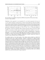
Fig. 20 and Fig. 21 show the smaller sampling interval make the pulse number of one
sampling interval become smaller, so that the speed error to speed command ratio will
become larger. The speed error is between -1 and +1 pulse per sampling interval.
In Fig. 21, the speed response is still stable with η = 0.5 , but more overshoot can be
investigated; owing to the fact that more learning rate induces more neural controller output
and get more overshoot. It can be investigated that the sampling time needs to be smaller,
then choosing a correspondent small learning rate. It is proven that the speed response of a
DC servo motor with the proposed direct neural controller is stable and accurate. The
simulation and experimental results show the speed error comes from speed sensor
characteristics, the measurement error is between -1 and +1 pulse per sampling interval. If
the resolution of encoder is improved, the accuracy of the control system will be increased.
The Artificial Neural Networks applied to servo control systems 325
The speed error is in the interval of 1 pulses/0.01s as the sampling time of 0.01s, but it is in
the interval of 1 pulses/0.001s as the sampling time of 0.001s. The step speed command is
assigned as 120 pulses/0.01s (150.72rad/s) with the sampling interval of 0.01s, and the step
speed command needs to be increased to 30pulses/ms (377rad/s) to keep the accuracy of
the speed measurement. Furthermore, we have to notice the normalization of the input
signals. From the experimental results, the input signals need to be normalized between +1
and A1. The learning rate should be determined properly depends on the sampling interval,
the smaller sampling interval can match the smaller learn rate, and increase the stability of

servo control system.

4. The Direct Neural Control Applied to Hydraulic Servo Control Systems

The electro-hydraulic servo systems are used in aircraft, industrial and robotic mechanisms.
They are always used for servomechanism to transmit large specific powers with low
control current and high precision. The electro-hydraulic servo system (EHSS) consists of
hydraulic supply units, actuators and an electro-hydraulic servo valve (EHSV) with its servo
driver. The EHSS is inherently nonlinear, time variant and usually operated with load
disturbance. It is difficult to determine the parameters of dynamic model for an EHSS.
Furthermore, the parameters are varied with temperature, external load and properties of
oil etc. The modern precise hydraulic servo systems need to overcome the unknown
nonlinear friction, parameters variations and load variations. It is reasonable for the EHSS to
use a neural network based adaptive control to enhance the adaptability and achieve the
specified performance.

4.1 Description of the electro-hydraulic servo control system
The EHSS is shown in Fig. 22 consists of hydraulic supply units, actuators and an electro-
hydraulic servo valve (EHSV) with its servo driver. The EHSV is a two-stage electro
hydraulic servo valve with force feedback. The actuators are hydraulic cylinders with
double rods.


Fig. 22. The hydraulic circuit of EHSS
326 New Developments in Robotics, Automation and Control
The application of the direct neural controller for EHSS is shown in Fig. 23, where y r is the
position command and p y is the actual position response.


Fig. 23. The block diagram of EHSS control system

A. The simplified servo valve model
The EHSV is a two-stage electro hydraulic servo valve with force feedback. The dynamic of
EHSV consists of inductance dynamic, torque motor dynamic and spool dynamic. The
inductance and torque motor dynamics are much faster than spool dynamic, it means the
major dynamic of EHSV determined by spool dynamic, so that the dynamic model of servo
valve can be expressed as:

(24)

: The displacement of spool
: The input voltage

B. The dynamic model of hydraulic cylinder
The EHSV is 4 ports with critical center, and used to drive the double rods hydraulic
cylinder. The leakages of oil seals are omitted and the valve control cylinder dynamic model
can be expressed as [8]:

(25)

x v: The displacement of spool
F L : The load force
X
P :The piston displacement
The Artificial Neural Networks applied to servo control systems 327
C. Direct Neural Control System
There are 5 hidden neurons in the proposed neural controller. The proposed DNC is shown
in Fig. 24 with a three layers neural network.

Fig. 24. The structure of proposed neural controller

The difference between command y r and the actual output position response y p is defined
as error e. The error e and its differential ė are normalized between A1 and +1 in the input
neurons before feeding to the hidden layer. In this study, the back propagation error term is
approximated by the linear combination of error and error:s differential. A tangent
hyperbolic function is designed as the activation function of the nodes in the output and
hidden layers. So that the net output in the output layer is bounded between A 1 and +1,
and converted into a bipolar analogous voltage signal through a D/A converter, then
amplified by a servo-amplifier for enough current to drive the EHSV. A square command is
assigned as the reference command in order to simulate the position response of the EHSS.
The proposed three layers neural network, including the hidden layer ( j ), output layer ( k )
and input layer ( i ) as illustrated in Fig. 24. The input signals e and ė
are normalized
between A 1 and +1, and defined as signals O i feed to hidden neurons. A tangent hyperbolic
function is used as the activation function of the nodes in the hidden and output layers. The
net input to node j in the hidden layer is

328 New Developments in Robotics, Automation and Control
(26)

the output of node j is

(27)

where β> 0 , the net input to node k in the output layer is

(28)

the output of node k is

(29)

The output O
k
of node k in the output layer is treated as the control input u
P
of the system
for a single-input and single-output system. As expressed equations, W
ji
represent the
connective weights between the input and hidden layers and W
kj
represent the connective
weights between the hidden and output layers θ
j
and θ
k
denote the bias of the hidden and
output layers, respectively. The error energy function at the Nth sampling time is defined as

(30)

where y
r N
, y
PN
and e
N
denote the the reference command, the output of the plant and the

error term at the Nth sampling time, respectively. The weights matrix is then updated
during the time interval from N to N+1.

(31)

where η is denoted as learning rate and α is the momentum parameter. The gradient of E
N
with respect to the weights W
kj
is determined by

(32)

and is defined as
The Artificial Neural Networks applied to servo control systems 329

(33)

where is difficult to be evaluated. The EHSS is a single-input and single-output
control system (i.e.,
n =1), in this study, the sensitivity of E
N
with respect to the network
output O
k
is approximated by a linear combination of the error and its differential shown as:

(34)

where K 3 and K 4 are positive constants. Similarly, the gradient of EN with respect to the

weights, W ji is determined by

(35)

where

(36)

The weight-change equations on the output layer and the hidden layer are

(37)

(38)
330 New Developments in Robotics, Automation and Control
where η is denoted as learning rate and α is the momentum parameter and can be
evaluated from Eq.(34) and (31), The weights matrix are updated during the time interval
from N to N+1 :

(39)

(40)

4.2 Numerical Simulation
An EHSS shown as Fig.1 with a hydraulic double rod cylinder controlled by an EHSV is
simulated. A LVDT of 1 V/m measured the position response of EHSS. The numerical
simulations assume the supplied pressure Ps = 70Kg
f
/ cm
2
, the servo amplifier voltage gain of

5, the maximum output voltage of 5V, servo valve coil resistance of 250 ohms, the current to
voltage gain of servo valve coil of 4 mA V (250 ohms load resistance), servo valve settling
time ≈ 20ms, the serve valve provides maximum output flow rate = 19.25 l /min under coil
current of 20mA and
ΔP of 70Kg
f
/ cm
2
condition. The spool displacement can be expressed by
percentage (%), and then the model of servo valve can be built as

(41)

or

(42)

The cylinder diameter =40mm, rod diameter=20mm, stroke=200mm, and the parameters of
the EHSS listed as following:


The Artificial Neural Networks applied to servo control systems 331
According to Eq(25), the no load transfer function is shown as

(43)

The direct neural controller is applied to control the EHSS shown as Fig. 24, and the time
responses for piston position are simulated. A tangent hyperbolic function is used as the
activation function, so that the neural network controller output is between -1 . This is
converted to be analog voltage between

-) Volt by a D/A converter and amplified in current
by a servo amplifier to drive the EHSV. The constants K
3 and K 4 are defined to be the
parameters for the linear combination of error and its differential, which is used to
approximate the BPE for weights update. A conventional PD controller with well-tuned
parameters is also applied to the simulation stage as a comparison performance. The square
signal with a period of 5
sec and amplitude of 0.1m is used as the command input. The
simulation results for PD control is shown in Fig. 25 and for DNC is shown in Fig. 26. Fig. 26
reveals that the EHSS with DNC track the square command with sufficient convergent
speed, and the tracking performance will become better and better by on-line trained. Fig. 27
shows the time response of piston displacement with 1200N force disturbance. Fig. 27 (a)
shows the EHSS with PD controller is induced obvious overshoot by the external force
disturbance, and Fig. 27 (b) shows the EHSS with the DNC can against the force disturbance
with few overshoot. From the simulation results, we can conclude that the proposed DNC is
available for position control of EHSS, and has favorable tracking characteristics by on-line
trained with sufficient convergent speed.


(a) Time response for piston displacement
332 New Developments in Robotics, Automation and Control

(b) Controller output
Fig. 25. The simulation results for EHSS with PD controller (Kp=7, Kd=1, Amplitude=0.1m
and period=5 sec)


(a) Time response for piston displacement
The Artificial Neural Networks applied to servo control systems 333

(b) Controller output
Fig. 26. The simulation results for EHSS with DNC (Amplitude=0.1m and period=5 sec )


(a) EHSS with PD controller
334 New Developments in Robotics, Automation and Control

(b) EHSS with DNC
Fig. 27. Simulation results of position response with 1200N force disturbance

4.3. Experiment
The EHSS shown in Fig. 22 is established for our experiment. A hydraulic cylinder with
200mm stroke, 20mm rod diameter and a 40mm cylinder diameter is used as the system
actuator. The Atchley JET-PIPE-206 servo valve is applied to control the piston position of
hydraulic cylinder. The output range of the neural controller is between -1 , and converted
to be the analog voltage between -5 Volt by a 12 bits bipolar DA /AD servo control interface,
It is amplified in current by a servo amplifier to drive the EHSV. A crystal oscillation
interrupt control interface provides an accurate 0.001 sec sample rate for real time control. A
square signal with amplitude of 10mm and period of 4 sec is used as reference input. Fig. 28
shows the EHSS disturbed by external load force, which is induced by load actuator with
operation pressure of 9 kg /cm
2

. Fig. 28 (a) shows the EHSS with PD controller is induced
obvious overshoot by the external force disturbance, and Fig. 28 (b) shows the EHSS with
the DNC can against the force disturbance with few overshoot. The experiment results show
the proposed DNC is available for position control of EHSS.


(a) EHSS with PD controller

The Artificial Neural Networks applied to servo control systems 335

(b) EHSS with DNC
Fig. 28. Experiment results of position response with the load actuator pressure of 9 kg /cm
2


The proposed DNC is applied to control the piston position of a hydraulic cylinder in an
EHSS., and the comparison of time responses for the PD control system is analyzed by
simulation and experiment. The results show that the proposed DNC has favorable
characteristic, even under external force load condition.

5. Conclusion

The conventional direct neural controller with simple structure can be implemented easily
and save more CPU time. But the Jacobian of plant is always not easily available. The DNC
using sign function for approximation of Jacobian is not sufficient to apply to servo control
system. The & adaptation law can increase the convergent speed effetely, but the
appropriate parameters always depend on try and error. It is not easy to evaluated the
appropriate parameters. The proposed self tuning type adaptive control can easily
determined the appropriate parameters. The DNC with the well-trained parameters will
enhance adaptability and improve the performance of the nonlinear control system.

6 References

D. Psaltis, A Sideris, and A. A. Yamamura (1988). A Multilayered Neural Network
Controller, IEEE Control System Magazine, v.8, pp. 17-21.
Y. Zhang, P. Sen, and G. E. Hearn (1995). An On-line Trained Adaptive Neural Controller,
IEEE Control System Magazine, v.15, pp. 67-75.
S. Weerasooriya and M. A. EI-Sharkawi Hearn (1991). Identification and Control of a DC

Motor Using Back-propagation Neural Networks, IEEE Transactions on Energy
Conversion, v.6, pp. 663-669.
A. Rubai and R. Kotaru (2000). Online Identification and Control of a DC Motor Using
Learning Adaptation of Neural Networks, IEEE Transactions on Industry
Applications, v.36, n.3.
336 New Developments in Robotics, Automation and Control
S. Weerasooriya and M. A. EI-Sharkawi (1993). Laboratory Implementation of A Neural
Network Trajectory Controller for A DC Motor, IEEE Transactions on Energy
Conversion, v.8, pp. 107-113.
G. Cybenko (1989). Approximation by Superpositions of A Sigmoidal Function, Mathematics
of Controls, Signals and Systems, v.2, n.4, pp. 303-314.
J. de Villiers and E. Barnard (1993). Backpropagation Neural Nets with One and Two
Hidden layers, IEEE Transactions on Neural Networks, v.4, n.1, pp. 136-141.
R. P. Lippmann (1987). An Introduction to Computing with Neural Nets, IEEE Acoustics,
Speech, and Signal Processing Magazine, pp. 4-22.
F. J. Lin and R. J. Wai (1998). Hybrid Controller Using Neural Network for PM Synchronous
Servo Motor Drive, Instrument Electric Engine Process Electric Power Application,
v.145, n.3, pp. 223-230.
Omatu, S. and Yoshioka, M. (1997). Self-tuning neuro-PID control and applications, IEEE,
International Conference on Systems, Man, and Cybernetics, Computational
Cybernetics and Simulation, Vol. 3.

Appendex: The simulation program
The simulation program for Example X.1 is listed as following=
1. Simulink block diagram


Fig. 1. The simulink program with S-function ctrnn3x

2. The content of S-function ctrnn3x(t, x, u, flag)

function [sys,x0,str,ts] = ctrnn3x(t,x,u,flag)
switch flag,
case 0,
[sys,x0,str,ts]=mdlInitializeSizes;
case 2,
sys=mdlUpdate(t,x,u);
case 3,
The Artificial Neural Networks applied to servo control systems 337
sys=mdlOutputs(t,x,u);
case {1,4,9}
sys=[];
otherwise
error(['Unhandled flag = ',num2str(flag)]);
end
function [sys,x0,str,ts]=mdlInitializeSizes
sizes = simsizes;
sizes.NumContStates = 0;
sizes.NumDiscStates = 21;
sizes.NumOutputs = 21;
sizes.NumInputs = 5;
sizes.DirFeedthrough = 1;
sizes.NumSampleTimes = 1;
sys = simsizes(sizes);
x0 = [rand(1)-0.5;rand(1)-0.5;rand(1)-0.5;rand(1)-0.5;rand(1)-0.5;
rand(1)-0.5;rand(1)-0.5;rand(1)-0.5;rand(1)-0.5;rand(1)-0.5;
rand(1)-0.5;rand(1)-0.5;rand(1)-0.5;rand(1)-0.5;rand(1)-0.5;
rand(1)-0.5;rand(1)-0.5;rand(1)-0.5;rand(1)-0.5;rand(1)-0.5;0.2];
%%%set the initial values for weights and states
%%%the initial values of weights randomly between -0.5 and +0.5
%%%the initial values of NN output assigned to be 0.2

str = [];
ts = [0 0];
function sys=mdlUpdate(t,x,u);
nv=0;
for j=1:5
for i=1:3
nv=nv+1;
w1(j,i)=x(nv);
end
end
k=1;
for j=1:5
nv=nv+1;
w2(k,j)=x(nv);
end
for j=1:5
jv(j)=w1(j,:)*[u(1);u(2);u(3)]; %u(1)=K1*e ,u(2)=K2*de/dt
%u(3)=1 is bias unity
ipj(j)=tanh(0.5*jv(j)); %outputs of hidden layer
end
kv(1)=w2(1,:)*ipj';
opk(1)=tanh(0.5*kv(1)); %output of output layer
for j=1:5
dk=(u(4)+u(5))*0.5*(1-opk(1)*opk(1));
%%%delta adaptation law, dk means delta K,u(4)=K3*e ,u(5)=K4*de/dt
dw2(1,j)=0.1*dk*ipj(j); %dw2 is weight update quantity for W2
end
for j=1:5
sm=0;
sm=sm+dk*w2(1,j);

sm=sm*0.5*(1-ipj(j)*ipj(j));
dj(j)=sm; %back propogation, dj means delta J
end
for j=1:5
for i=1:3
338 New Developments in Robotics, Automation and Control
dw1(j,i)=0.1*dj(j)*u(i); %dw1 is weight update quantity for W1
end
end
for j=1:5
w2(1,j)=w2(1,j)+dw2(1,j); %weight update
for i=1:3
w1(j,i)=w1(j,i)+dw1(j,i); %weight update
end
end
nv=0;
for j=1:5
for i=1:3
nv=nv+1;
x(nv)=w1(j,i); %assign w1(1)-w1(15) to x(1)-x(15)
end
end
k=1;
for j=1:5
nv=nv+1;
x(nv)=w2(k,j); %assign w2(1)-w2(5) to x(16)-x(20)
end
x(21)=opk(1); %assign output of neural network to x(21)
sys=x; %Assign state variable x to sys
function sys=mdlOutputs(t,x,u)

for i=1:21
sys(i)=x(i);
end


19

Linear Programming in Database

Akira Kawaguchi and Andrew Nagel
Department of Computer Science, The City College of New York. New York, New York
United States of America

Keywords: linear programming, simplex method, revised simplex method, database, stored
procedure.

Abstract

Linear programming is a powerful optimization technique and an important field in the
areas of science, engineering, and business. Large-scale linear programming problems arise
in many practical applications, and solving these problems requires an integration of data-
analysis and data-manipulation capabilities. Database technology has become a central
component of today’s information systems. Almost every type of organization is now using
database systems to store, manipulate, and retrieve data. Nevertheless, little attempt has
been made to facilitate general linear programming solvers for database environments.
Dozens of sophisticated tools and software libraries that implement linear programming
models can be found. But, there is no database-embedded linear programming tool
seamlessly and transparently utilized for database processing. The focus of the study in this
chapter is to fill this technical gap between data analysis and data manipulation, by solving
large-scale linear programming problems with applications built on the database

environment. Specifically, this chapter studies the representation of the linear programming
model in relational structures, as well as the computational method to solve the linear
programming problems. We have developed a set of ready to use stored procedures to solve
general linear programming problems. A stored procedure is a group of SQL statements,
precompiled and physically stored within a database, thereby having complex logic run
inside the database. We show versions of procedures in the open-source MySQL database
and commercial Oracle database system. The experiments are performed with several
benchmark problems extracted from the Netlib library. Foundations for and preliminary
experimental results of this study are presented.
*


1. Introduction


*
This work has been partly supported by New York State Department of Transportation
and New York City Department of Environment Protection.


New Developments in Robotics, Automation and Control

340
Linear programming is a powerful technique for dealing with the problem of allocating
limited resources among competing activities, as well as other problems having a similar
mathematical formulation (Winston, 1994, Richard, 1991, Walsh, 1985). It has become an
important field of optimization in the areas of science and engineering and has become a
standard tool of great importance for numerous business and industrial organizations. In
particular, large-scale linear programming problems arise in practical applications such as
logistics for large spare-parts inventory, revenue management and dynamic pricing, finance,

transportation and routing, network design, and chip design (Hillier and Lieberman, 2001).

While these problems inevitably involve the analysis of a large amount of data, there has
been relatively little work addressing this in the database context. Little serious attempt has
been made to facilitate data-driven analysis with data-oriented techniques. In today’s
marketplace, dozens of sophisticated tools and software libraries that implement linear
programming models can be found. Nevertheless, these products do not work with
database systems seamlessly. They rather require additional software layers built on top of
databases to extract and transfer data in the databases. The focus of our study gathered here
is to fill this technical gap between data analysis and data manipulation by solving large-
scale linear programming problems with applications built on the database environment.

In mathematics, linear programming problems are optimization problems in which the
objective function to characterize optimality of a problem and the constraints to express
specific conditions for that problem are all linear (Hillier and Lieberman, 2001, Thomas H.
Cormen and Stein, 2001). Two families of solution methods, so-called simplex methods
(Dantzig, 1963) and interior-point methods (Karmarkar, 1984), are in wide use and available as
computer programs today. Both methods progressively improve series of trial solutions by
visiting edges of the feasible boundary or the points within the interior of the feasible
region, until a solution is reached that satisfies the constraints and cannot be improved. In
fact, it is known that large problem instances render even the best of codes nearly unusable
(Winston, 1994). Furthermore, the program libraries available today are found outside the
standard database environment, thus mandating the use of a special interface to interact
with these tools for linear programming computations.

This chapter gives a detailed account of the methodology and technical issues related to
general linear programming in the relational (or object-relational) database environment.
Our goal is to find a suitable software platform for solving optimization problems on the
extension of a large amount of information organized and structured in the relational
databases. In principle, whenever data is available in a database, solving such problems

should be done in a database way, that is, computations should be closed in the world of the
database. There is a standard database language, ANSI SQL, for the manipulation of data in
the database, which has grown to a level comparable to most ordinary programming or
scripting languages. Eliminating reliance on a commercial linear programming package,
thus eliminating the overhead of data transfer between database and package is what we
hope to achieve.

There are also the issues of trade-off. A basic nature of linear programming is a collection of
matrices defining a problem and a sequence of algebraic operations repeatedly applied to
Linear Programming in Database

341
these matrices, hence giving a perfect match for array-based programming in scientific
computations. In general, the relational database is not designed for matrix operations like
solving linear programming problems. Indeed, realizing matrix operations on top of the
standard relational (or object-relational) structure is non-trivial. On the other hand, at the
heart of the database system is the ability to effectively manage resources coupled with an
efficient data access mechanism. The response to user is made by the best available sequence
of operations, or so-called optimized queries, on the actual data. When handling extremely
large matrices, the system probably gives a performance advantage over the unplanned or
ad hoc execution of the program causing an insatiable use of virtual memory (thus causing
thrashing) for the disposition of arrays.

In this chapter, implementation techniques and key issues for this development are studied
extensively. A model suitable to capture the dynamics of linear programming computations
is incorporated into the aimed development, by way of realizing a set of procedural
interfaces that enables a standard database language to define problems within a database
and to derive optimal solutions for those problems without requiring users to write detailed
program statements. Specifically, we develop two sets of ready to use stored procedures to
solve general linear programming problems. A stored procedure is a group of SQL

statements, precompiled and physically stored within a database (Gulutzan and Pelzer,
1999, Gulutzan, 2007). It forms a logical unit to encapsulate a set of database operations,
defined with an application program interface to perform a particular task, thereby having
complex logic run inside the database. The exact implementation of a stored procedure
varies from one database to another, but is supported by most major database vendors. To
this end, we will show implementations using MySQL open-source database system and
freely available Oracle Express Edition selected from the commercial domain. Our choice of
these popular database environments is to justify the feasibility of concepts and to draw
comparisons of their usability.

The rest of this chapter is organized as follows: Section 2 defines the linear programming
model and introduces our approach to express the model in the relational database. Section
3 presents details of developed simulation system and experimental performance studies.
Section 4 discusses related work, and Section 5 concludes our work gathered in this chapter.

2. Fundamentals

A linear programming problem consists of a collection of linear inequalities on a number of
real variables and a fixed linear function to maximize or minimize. In this section, we
summarize the principle technical issues in formulating the problem and some solution
method in the relational database environment.

2.1 Linear Programming Principles
Consider the matrix notation expressed in the set of equations (1) below. The standard form
of the linear programming problem is to maximize an objective function Z = c
T
x, subject to
the functional constraints of Ax ≤ b and non-negativity constraints of x ≥ 0, with 0 in this
case being the n-dimensional zero column vector. A coefficient matrix A and column vectors
c, b, and x are defined in the obvious manner such that each component of the column

New Developments in Robotics, Automation and Control

342
vector Ax is less than or equal to the corresponding component of the column vector b. But
all forms of linear programming problems arise in practice, not just ones in the standard
form, and we must deal with issues such as minimization objectives, constraints of the form
Ax ≥ b or Ax = b, variables ranging in negative values, and so on. Adjustments can be made
to transform every non-standard problem into the standard form. So, we limit our
discussion to the standard form of the problem.

⎥
⎥
⎥
⎥
⎥
⎦
⎤
⎢
⎢
⎢
⎢
⎢
⎣
⎡
=
⎥
⎥
⎥
⎥
⎥

⎦
⎤
⎢
⎢
⎢
⎢
⎢
⎣
⎡
=
⎥
⎥
⎥
⎥
⎥
⎦
⎤
⎢
⎢
⎢
⎢
⎢
⎣
⎡
=
⎥
⎥
⎥
⎥
⎥

⎦
⎤
⎢
⎢
⎢
⎢
⎢
⎣
⎡
=
⎥
⎥
⎥
⎥
⎥
⎦
⎤
⎢
⎢
⎢
⎢
⎢
⎣
⎡
=
mnmm
n
n
nnn
aaa

aaa
aaa
b
b
b
c
c
c
x
x
x
L
MMM
L
L
M
MMM
21
22221
11211
2
1
2
1
2
1
0
0
0
A0

bcx
,
,,,

(1)

The goal is to find an optimal solution, that is, the most favorable values of the objective
function among feasible ones for which all the constraints are satisfied. The simplex method
(Dantzig, 1963) is an algebraic iterative procedure where each round of computation
involves solving a system of equations to obtain a new trial solution for the optimality test.
The simplex method relies on the mathematical property that the objective function’s
maximum must occur on a corner of the space bounded by the constraints of the feasible
region.

To apply the simplex method, linear programming problems must be converted into a so-
called augmented form, by introducing non-negative slack variables to replace non-equalities
with equalities in the constraints. The problem can then be rewritten in the following form:

[]
⎥
⎦
⎤
⎢
⎣
⎡
=
⎥
⎥
⎥
⎦

⎤
⎢
⎢
⎢
⎣
⎡
⎥
⎦
⎤
⎢
⎣
⎡
−
≥
⎥
⎦
⎤
⎢
⎣
⎡
=
⎥
⎦
⎤
⎢
⎣
⎡
=
⎥
⎥

⎥
⎥
⎥
⎥
⎦
⎤
⎢
⎢
⎢
⎢
⎢
⎢
⎣
⎡
+
+
+
b
x
x
IA0
0c
0
x
x
b
x
x
IAx
s

0
1
2
1
s
T
ss
mn
n
n
Z
x
x
x
,,
,
M

(2)

In equations (2) above, x ≥ 0, a column vector of slack variables x
s
≥ 0, and I is the m × m
identity matrix. Following the convention, the variables set to zero by the simplex method
are called nonbasic variables and the others are called basic variables. If all of the basic
variables are non-negative, the solution is called a basic feasible solution. Two basic feasible
solutions are adjacent if all but one of their nonbasic variables are the same. The spirit of the
simplex method utilizes a rule for generating from any given basic feasible solution a new
one differing from the old in respect of just one variable.

Thus, moving from the current basic feasible solution to an adjacent one involves switching
one variable from nonbasic to basic and vice versa for one other variable. This movement
involves replacing one nonbasic variable (called entering basic variable) by a new one (called
Linear Programming in Database

343
leaving basic variable) and identifying the new basic feasible solution. The simplex algorithm
is summarized as follows:

Simplex Method:
1. Initialization: transform the given problem into an augmented form, and select original
variables to be the nonbasic variables (i.e., x = 0), and slack variable to be the basic
variables (i.e., x
s
= b).
2. Optimality test: rewrite the objective function by shifting all the nonbasic variables to
the right-hand side, and see if the sign of the coefficient of every nonbasic variable is
positive, in which case the solution is optimal.
3. Iterative Step:
3.1 Selecting an entering variable: as the nonbasic variable whose coefficient is largest in
the rewritten objective function used in the optimality test.
3.2 Selecting a leaving variable: as the basic variable that reaches zero first when the
entering basic variable is increased, that is, the basic variable with the smallest upper
bound.
3.3 Compute a new basic feasible solution: by applying the Gauss-Jordan method of
elimination, and apply the above optimality test.

2.2 Revised Simplex Method
The computation of the simplex method can be improved by reducing the number of
arithmetic operations as well as the amount of round-off errors generated from these

operations (Hillier and Lieberman, 2001, Richard, 1991, Walsh, 1985). Notice that n nonbasic
variables from among the n + m elements of [x
T
,x
s
T
]
T
are always set to zero. Thus,
eliminating these n variables by equating them to zero leaves a set of m equations in m
unknowns of the basic variables. The spirit of the revised simplex method (Hillier and
Lieberman, 2001, Winston, 1994) is to preserve only the pieces of information relevant at
each iteration, which consists of the coefficients of the nonbasic variables in the objective
function, the coefficients of the entering basic variable in the other equations, and the right-
hand side of the equations.

Specifically, consider the equations (3) below. The revised method attempts to derive a basic
(square) matrix B of size m × m by eliminating the columns corresponding to coefficients of
nonbasic variables from [A, I] in equations (2). Furthermore, let c
B
T
be the vector obtained
by eliminating the coefficients of nonbasic variables from [c
T
, 0
T
]
T
and reordering the
elements to match the order of the basic variables. Then, the values of the basic variables

become B
-1
b and Z = c
B
T
B
-1
b. The equations (2) become equivalent with equations (3) after
any iteration of the simplex method.

⎥
⎦
⎤
⎢
⎣
⎡
=
⎥
⎥
⎥
⎦
⎤
⎢
⎢
⎢
⎣
⎡
⎥
⎦
⎤

⎢
⎣
⎡
−
=
−
−
−−
−−
⎥
⎥
⎥
⎥
⎥
⎥
⎥
⎥
⎥
⎥
⎦
⎤
⎢
⎢
⎢
⎢
⎢
⎢
⎢
⎢
⎢

⎢
⎣
⎡
bB
bBc
x
x
BAB0
BccABc
B
B
BB
1
1T
11
1T1T
21
22221
11211
1
s
T
mmmm
m
m
BBB
BBB
BBB
Z
,

L
MMM
L
L

(3)
New Developments in Robotics, Automation and Control

344

This means that only B
-1
needs to be derived to be able to calculate all the numbers used in
the simplex method from the original parameters of A, b, c
B
—providing efficiency and
numerical stability.

2.3 Relational Representation
A relational model provides a single way to represent data as a two-dimensional table or a
relation. An n-ary relation being a subset of the Cartesian product of n domains has a
collection of rows called tuples. Implementions of the simplex and revised simplex methods
must locate the exact position of the values for the equations and variables of the linear
programming problem to solve. However, the position of the tuples in the table is not
relevant in the relational model. By definition, tuple ordering and matrix handling are
beyond the standard relational features, and these are the most important issues that need to
be addressed to implement the linear programming solver within the database using the
simplex method. We will explore two distinct methods for representing matrices in the
relational model.

Simplex calculations are most conveniently performed with the help of a series of tables
known as simplex tableaux (Dantzig, 1963, Hillier and Lieberman, 2001). A simplex tableau is
a table that contains all the information necessary to move from one iteration to another
while performing the simplex method. Let xB be a column vector of m basic variables
obtained by eliminating the nonbasic variables from x and xs. Then, the initial tableau can be
expressed as,

⎥
⎥
⎥
⎥
⎦
⎤
⎢
⎢
⎢
⎢
⎣
⎡
−
bIA0x
0c
B
01
T
Z

(4)

The algebraic treatment based on the revised simplex method (Hillier and Lieberman, 2001,

William H. Press and Flannery, 2002) derives the values at any iteration of the simplex
method as,

⎥
⎥
⎥
⎥
⎦
⎤
⎢
⎢
⎢
⎢
⎣
⎡
−−−
−−−
−
bBBAB0x
bBcBccABc
B
BBB
111
1T1T1T
1
T
Z

(5)

For the matrices expressed (4) and (5), the first two column elements do not need to be
stored in persistent memory. Thus, the simplex tableau can be a table using the rest of the
three column elements in the relational model. Creating table instances as simplex tableaux
is perhaps the most straighforward way. Indeed, our MySQL implementation in the next
section uses this representation, in which a linear programming problem in the augmented
form (equations (2)) can be seen as a relation:

tableau(id
, x1,x2, · · · xn, rhs)

Linear Programming in Database

345
A variable of the constraints and the objective function becomes an attribute of the relation,
together with the right hand side that becomes the rhs column on the table. The id column
serves as a
key that can uniquely determine every variable of the constraints and of the
objective function in the tuple. A constraint of the linear programming problem in the
augmented form is identified by a unique positive integer value ranging from 1 to
n in the id
column, where
n is the number of constraints for the problem plus the objective function.
Thus by applying relational operations, it is feasible to know the position of every constraint
and variable for a linear programming problem, and to proceed with the matrix operations
necessary to implement the simplex algorithm. See Figure 1 for the table instance populated
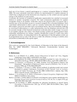
with a simple example.


Fig. 1. Two representations of the initial simplex tableau in the relational database

The main drawback of this design is a fixed structure of table. An individual table needs to
be created for each problem, and the cost of defining (and dropping) table becomes part of
the process implementing the simplex method. The number of tables in the database will
increase as the collection of problems to solve accumulates. This may cause administrative
strain for database management. Subtle issues arise in the handling of large-scale problems.
The table maps to the full instance of the matrix even if the problem has sparsely populated
non-zero data. Thousands of zero values (or null values specific to database) held in a tuple
pile up a significant amount of space. Besides, a tuple of a large number of non-zero values
is problematic because the physical record holding such a tuple may not fit into a disk block.
Accessing a spanned record over multiple disk blocks is time-consuming.

As an alternative to the table-as-tableaux structure, element-by-element represenation can
be considered. The simplex tableaux are decomposed to a collection of values, each of which
is a tuple consisting of a tableau id, a row position, a column position, and a value in the
specified position. This is to say that the table no longer possesses the shape of a tableau but
has the information to locate every element in the tableau. Missing elements are zeros, thus
space efficient for sparse contents. A single table can gather all the problem instances, in that
the elements in the specific tableau are found by the use of the tableau id. The size of the
tuple is small because there are only four attributes in the tuple. In return, there is a time
New Developments in Robotics, Automation and Control

346
overhead for finding a specific element in the table. Our Oracle XE implementation detailed
in the next section utilizes this representation.

3. System Development

The availability of real-time databases capable of accepting and solving linear programming
problems helps us examine the effectiveness and practical usability in integrating linear
programming tools into the database environment. Towards this end, a general linear

programming solver is developed on top of the
de facto standard database environment,
with the combination of a PHP application for the front-end and a MySQL or Oracle
application for the backend. Note that the implementation of this linear programming solver
is strictly within the database technology, not relying on any outside programming
language.


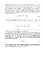
Fig. 2. Architecture of the implemented linear programming solver
The systems architecture is summarized in Figure 2. The PHP front-end enables the user to
input the number of variables and number of constraints of the linear programming
problem to solve. With these values, it generates a dynamic Web interface to accept the
values of the objective function and the values of the constraining equations. The Web
interface also allows the user to upload a file in a MPS (Mathematical Programming System)
format that defines a linear programming problem. The MPS file format serves as a standard
for describing and archiving linear programming and mixed integer programming
problems (Organization, 2007). A special program is built to convert MPS data format into
SQL statements for populating a linear programming instance. The main objective of this
development is to obtain benchmark performances for large-scale linear programming
problems.
Linear Programming in Database

347
The MySQL and Oracle back-ends perform iterative computations by the use of a set of
stored procedures precompiled and integrated into the database structure. The systems
encapsulate an API for processing a simplex method that requires the execution of several
SQL queries to produce a solution. The input and output of the system are shown in Figure
3 in which each table of the right figure represents the tableau containing the values resulted
from each iteration of the simplex method. The system presents successive transformations
and optimal solution if it exists.

Fig. 3. Simplex method iterations and optimal solution
3.1 Stored Procedure Implementation MySQL
Stored procedures can have direct accesses to the data in the database, and run their steps
directly and entirely within the database. The complex logic runs inside the database engine,
thus faster in processing requests because numerous context switches and a great deal of
network traffic can be eliminated. The database system only needs to send the final results
back to the user, doing away with the overhead of communicating potentially large
amounts of interim data back and forth (Gulutzan, 2007, Gulutzan and Pelzer, 1999).