New Developments in Robotics, Automation and Control 2009 Part 14 ppt

Active Vibration Control of a Smart Beam by Using a Spatial Approach 383
presented by Moheimani (Moheimani, 2000a) which considers adding a correction term that
minimizes the weighted spatial
2
H norm of the truncation error. The additional correction
term had a good improvement on low frequency dynamics of the truncated model.
Moheimani (2000d) and Moheimani et al. (2000c) developed their corresponding approach
to the spatial models which are obtained by different analytical methods. Moheimani
(2006b) presented an application of the model correction technique on a simply-supported
piezoelectric laminate beam experimentally. However, in all those studies, the damping in
the system was neglected. Halim (2002b) improved the model correction approach with
damping effect in the system. This section will give a brief explanation of the model
correction technique with damping effect based on those previous works (Moheimani,
2000a, 2000c and 2000d) and for more detailed explanation the reader is advised to refer to
the reference (Moheimani, 2003).

Recall the transfer function of the system from system input to the beam deflection
including N number of modes given in equation (8). The spatial system model expression
includes N number of resonant modes assuming that N is sufficiently large. The controller
design however interests in the first few vibration modes of the system, say M number of
lowest modes. So the truncated model including first M number of modes can be expressed
as:

22
1
()
(,)
2
φ
ξ
ωω

=
=
∑
++
M
ii
M
i
ii i
Pr
Gsr
ss
(12)

where
M
N<<
. This truncation may cause error due to the removed modes which can be
expressed as an error system model,
(,)
E
sr
:


22
1
(,) (,) (,)
()

2
φ
ξ
ωω
=+
=
−
=
∑
++
NM
N
ii
iM
ii i
Esr G sr G sr
Pr
ss
(13)

In order to compensate the model truncation error, a correction term should be added to the
truncated model (Halim, 2002b):

(,) (,) ()
=
+
CM
Gsr G sr Kr
(14)

where (,)
C
Gsr and ()Kr are the corrected transfer function and correction term,
respectively.
The correction term
()Kr involves the effects of removed modes of the system on the
frequency range of interest, and can be expressed as:
384 New Developments in Robotics, Automation and Control

1
() ()
φ
=+
=
∑
N
ii
iM
Kr rk (15)

where
i
k is a constant term. The reasonable value of
i
k should be determined by keeping
the difference between (,)
N
Gsr and (,)
C
Gsr to be minimum, i.e. corrected system

model should approach more to the higher ordered one given in equation (8). Moheimani
(2000a) represents this condition by a cost function,
J , which describes that the spatial
2
H
norm of the difference between (, )
N
Gsr and (,)
C
Gsr should be minimized:

{
}
2
2
(,) (,) (,)
=
<< − >>
NC
JWsrGsrGsr
(16)

The notation
2
2
<< >> represents the spatial
2
H norm of a system where spatial norm
definitions are given in (Moheimani, 2003).
(,)Wsr

is an ideal low-pass weighting
function distributed spatially over the entire domain
R
with its cut-off frequency
c
ω

chosen to lie within the interval (
M
ω
,
1M
ω
+
) (Moheimani, 2000a). That is:

()
1
1
1 - ,
(,)
0
,
ωωω
ω
ωωω
+
+
<< ∈
⎧

⎫
=
⎨
⎬
⎩⎭
∈
cc
cMM
rR
Wj r
elsewhere
and
(17)

where
M
ω
and
1M
ω
+
are the natural frequencies associated with mode number
M
and
1
M
+
, respectively. Halim (2002b) showed that, by taking the derivative of cost function
J with respect to
i

k and using the orthogonality of eigenfunctions, the general optimal
value of the correction term, so called
opt
i
k , for the spatial model of resonant systems,
including the damping effect, can be shown to be:

222
22 22
21
11
ln
4
121
ωωω ξω
ωω
ξωωωξω
⎧
⎫
+−+
⎪
⎪
=
⎨
⎬
−−−+
⎪
⎪
⎩⎭
opt

cci ii
i i
ci
icciii
kP
(18)

An interesting result of equation (18) is that, if damping coefficient is selected as zero for
each mode, i.e. undamped system, the resultant correction term is equivalent to those given
Active Vibration Control of a Smart Beam by Using a Spatial Approach 385
in references (Moheimani, 2000a, 2000c and 2000d) for an undamped system. Therefore,
equation (18) can be represented as not only the optimal but also the general expression of
the correction term.

So, following the necessary mathematical manipulations, one will obtain the corrected
system model including the effect of out-of-range modes as:


22
1
222
22 22
1
()
(,)
2
21
11
( ) ln
4

121
φ
ξω ω
ωωω ξω
φ
ωω
ξωωωξω
=
=+
=
∑
++
⎧
⎫
⎧⎫
+−+
⎪
⎪⎪⎪
+
∑
⎨
⎨⎬⎬
−−−+
⎪
⎪⎪⎪
⎩⎭
⎩⎭
M
ii
C

i
ii i
N
cci ii
i i
iM
ci
icciii
Pr
Gsr
ss
rP
(19)

Consider the cantilevered smart beam depicted in Fig.1 with the structural properties given
at Table 1. The beginning and end locations of the PZT patches 0.027
1
r = m and
0.077
2
r = m away from the fixed end, respectively. Note that, although the actual length of
the passive beam is 507mm, the effective length, or span, reduces to 494mm due to the
clamping in the fixture.

Aluminum Passive
Beam
PZT
Length
= 0.494Lm
b

= 0.05Lm
p

Width
w = 0.051m
b
w = 0.04m
p

Thickness
t = 0.002m
b
t = 0.0005m
p

Density 3
ρ
= 2710k
g
/m
b

3
ρ
= 7650k
g
/m
p

Young’s Modulus
E = 69GPa
b

E = 64.52GPa
p

Cross-sectional Area -4 2
A = 1.02 ×10 m
b

-4 2
A
=0.2×10 m
p

Second Moment of Area -11 4
I = 3.4 × 10 m
b

-11 4
I = 6.33 × 10 m
p

Piezoelectric charge constant - -12
d = -175 ×10 m/V
31

Table 1. Properties of the Smart Beam

386 New Developments in Robotics, Automation and Control
The system model given in equation (8) includes N number of modes of the smart beam,
where as
N gets larger, the model becomes more accurate. In this study, first 50 flexural
resonance modes are included into the model (i.e.
N=50) and the resultant model is called
the full order model:

50
50
22
1
()
(,)
2
φ
ξ
ωω
=
=
∑
++
ii
i
ii i
Pr
Gsr
ss
(20)

However, the control design criterion of this study is to suppress only the first two flexural
modes of the smart beam. Hence, the full order model is directly truncated to a lower order
model, including only the first two flexural modes, and the resultant model is called
the
truncated model
:

2
2
22
1
()
(,)
2
φ
ξ
ωω
=
=
∑
++
ii
i
ii i
Pr
Gsr
ss
(21)

As previously explained, the direct model truncation may cause the zeros of the system to

perturb, which consequently affect the closed-loop performance and stability of the system
considered (Clark, 1997). For this reason, the general correction term, given in equation (18),
is added to the truncated model and the resultant model is called
the corrected model:


2
22
1
222
50
22 22
3
()
(,)
2
21
11
( ) ln
4
121
φ
ξω ω
ωωω ξω
φ
ωω
ξωωωξω
=
=
=

∑
++
⎧
⎫
⎧⎫
+−+
⎪
⎪⎪⎪
+
∑
⎨
⎨⎬⎬
−−−+
⎪
⎪⎪⎪
⎩⎭
⎩⎭
ii
C
i
ii i
cci ii
ii
i
ci
icciii
Pr
Gsr
ss
rP

(22)

where the cut-off frequency, based on the selection criteria given in equation (17), is taken
as:

(
)
23
/2
ωωω
=+
c
(23)

The assumed-modes method gives the first three resonant frequencies of the smart beam as
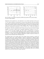
shown in Table 2. Hence, the cut-off frequency becomes 79.539 Hz. The performance of
model correction for various system models obtained from different measurement points
along the beam is shown in Fig.3 and Fig.4.

Active Vibration Control of a Smart Beam by Using a Spatial Approach 387
Resonant Frequencies Value (Hz)
1
ω

6.680
2
ω

41.865
3

ω

117.214
Table 2. First three resonant frequencies of the smart beam

The error between full order model-truncated model, and the error between full order
model-corrected model, so called the error system models
FT
E
−
and
FC
E
−
, allow one to
see the effect of model correction more comprehensively.

(,) (,)
−
=−
FT N M
EGsrGsr (24)

(,) (,)
−
=−
FC N C
EGsrGsr (25)

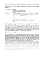
The frequency responses of the error system models are shown in Fig.5 and Fig.6. One can

easily notice from the aforementioned figures that, the error between the full order and
corrected models is less than the error between the full order and truncated ones in a wide
range of the interested frequency bandwidth. That is, the model correction minimizes error
considerably and makes the truncated model approach close to the full order one. The error
between the full order and corrected models is smaller at low frequencies and around 50 Hz
it reaches a minimum value. As a result, model correction reduces the overall error due to
model truncation, as desired.

In this study, the experimental system models based on displacement measurements were
obtained by nonparametric identification. The smart beam was excited by piezoelectric
patches with sinusoidal chirp signal of amplitude 5V within bandwidth of 0.1-60 Hz, which
covers the first two flexural modes of the smart beam. The response of the smart beam was
acquired via laser displacement sensor from specified measurement points. Since the
patches are relatively thin compared to the passive aluminum beam, the system was
considered as 1-D single input multi output system, where all the vibration modes are
flexural modes. The open loop experimental setup is shown in Fig.7.

In order to have more accurate information about spatial characteristics of the smart beam,
17 different measurement points, shown in Fig.8, were specified. They are defined at 0.03m
intervals from tip to the root of the smart beam.

The smart beam was actuated by applying voltage to the piezoelectric patches and the
transverse displacements were measured at those locations. Since the smart beam is a
spatially distributed system, that analysis resulted in 17 different single input single output
system models where all the models were supposed to share the same poles. That kind of
388 New Developments in Robotics, Automation and Control
analysis yields to determine uncertainty of resonance frequencies due to experimental
approach. Besides, comparison of the analytical and experimental system models obtained
for each measurement points was used to determine modal damping ratios and the
uncertainties on them. That is the reason why measurement from multiple locations was

employed. The rest of this section presents the comparison of the analytical and
experimental system models to determine modal damping ratios and clarify the
uncertainties on natural frequencies and modal damping ratios.

Consider the experimental frequency response of the smart beam at point
b
r = 0.99L .
Because experimental frequency analysis is based upon the exact dynamics of the smart
beam, the values of the resonance frequencies determined from experimental identification
were treated as being more accurate than the ones obtained analytically, where the
analytical values are presented in Table 2. The first two resonance frequencies were
extracted as 6.728 Hz and 41.433 Hz from experimental system model. Since the analytical
and experimental models should share the same resonance frequencies in order to coincide
in the frequency domain, the analytical model for the location
b
r = 0.99L was coerced to
have the same resonance frequencies given above. Notice that, the corresponding
measurement point can be selected from any of the measurement locations shown in Fig.8.
Also note that, the analytical system model is the corrected model of the form given in
equation (22). The resultant frequency responses are shown in Fig.9.

The analytical frequency response was obtained by considering the system as undamped.
The point
b
r = 0.99L was selected as measurement point because of the fact that the free end
displacement is significant enough for the laser displacement sensor measurements to be
more reliable. After obtaining both experimental and analytical system models, the modal
damping ratios were tuned until the magnitude of both frequency responses coincide at
resonance frequencies, i.e.:

(,) (,)
ωω
λ
=
−
<
i
EC
Gsr Gsr (26)

where (,)
E
Gsr is the experimental transfer function and
λ
is a very small constant term.
Similar approach can be employed by minimizing the 2-norm of the differences of the
displacements by using least square estimates (Reinelt, 2002).

Fig.10 shows the effect of tuning modal damping ratios on matching both system models in
frequency domain where
λ
is taken as 10
-6
. Note that each modal damping ratio can be
tuned independently.

Consequently, the first two modal damping ratios were obtained as 0.0284 and 0.008,
respectively. As the resonance frequencies and damping ratios are independent of the
location of the measurement point, they were used to obtain the analytical system models of
the smart beam for all measurement points. Afterwards, experimental system identification

was again performed for each point and both system models were again compared in
Active Vibration Control of a Smart Beam by Using a Spatial Approach 389
frequency domain. The experimentally identified flexural resonance frequencies and modal
damping ratios were determined by tuning for each point and finally a set of resonance
frequencies and modal damping ratios were obtained. The amount of uncertainty on
resonance frequencies and modal damping ratios can also be determined by spatial system
identification. There are different methods which can be applied to determine the
uncertainty and improve the values of the parameters
ω
and
ξ
such as boot-strapping
(Reinelt, 2002). However, in this study the uncertainty is considered as the standard
deviation of the parameters and the mean values are accepted as the final values, which are
presented at Table 3.


1
ω
(Hz)
2
ω
(Hz)
1
ξ

2
ξ

Mean 6.742 41.308 0.027 0.008

Standard Deviation 0.010 0.166 0.002 0.001
Table 3. Mean and standard deviation of the first two resonance frequencies and modal
damping ratios

For more details about spatial system identification one may refer to (Kırcalı, 2006a).
The estimated and analytical first two mode shapes of the smart beam are given in Fig.11
and Fig.12, respectively (Kırcalı, 2006a).


Fig. 3. Frequency response of the smart beam at
r = 0.14L
b

390 New Developments in Robotics, Automation and Control


Fig. 4. Frequency response of the smart beam at
r = 0.99L
b

Fig. 5. Frequency responses of the error system models at r = 0.14L
b
Active Vibration Control of a Smart Beam by Using a Spatial Approach 391
Fig. 6. Frequency responses of the error system models at r = 0.99L
b

Fig. 7. Experimental setup for the spatial system identification of the smart beam

392 New Developments in Robotics, Automation and Control

Fig. 8. The locations of the measurement points


Fig. 9. Analytical and experimental frequency responses of the smart beam at r=0.99
L
b

Active Vibration Control of a Smart Beam by Using a Spatial Approach 393

Fig. 10. Experimental and tuned analytical frequency responses at r=0.99
L
b



Fig. 11. First mode shape of the smart beam
394 New Developments in Robotics, Automation and Control

Fig. 12. Second mode shape of the smart beam

4. Spatial H
∞
Control Technique

Obtaining an accurate system model lets one to understand the system dynamics more
clearly and gives him the opportunity to design a consistent controller. Various control
design techniques have been developed for active vibration control like
∞
H or
2

H methods
(Francis, 1984 and Doyle, 1989).
The effectiveness of
∞
H controller on suppressing the vibrations of a smart beam due to its
first two flexural modes was studied by Yaman et al. (2001) and the experimental
implementation of the controller was presented (2003). By means of
∞
H theory, an additive
uncertainty weight was included to account for the effects of truncated high frequency
modes as the model correction. Similar work has been done for suppressing the in-vacuo
vibrations due to the first two modes of a smart fin (Yaman, 2002a, 2002b) and the
effectiveness of the
∞
H control technique in the modeling of uncertainties was also shown.
However,
∞
H theory does not take into account the multiple sources of uncertainties,
which yield unstructured uncertainty and increase controller conservativeness, at different
locations of the plant. That problem can be handled by using the μ-synthesis control design
method (Nalbantoğlu, 1998; Ülker, 2003 and Yaman, 2003).
Active Vibration Control of a Smart Beam by Using a Spatial Approach 395
Whichever the controller design technique is employed, the major objective of vibration
control of a flexible structure is to suppress the vibrations of the first few modes on well-
defined specific locations over the structure. As the flexible structures are distributed
parameter systems, the vibration at a specific point is actually related to the vibration over
the rest of the structure. As a remedy, minimizing the vibration over entire structure rather
than at specific points should be the controller design criterion. The cost functions
minimized as design criteria in standard
2

H or
∞
H control methodologies do not contain
any information about the spatial nature of the system. In order to handle this absence,
Moheimani and Fu (1998c), and Moheimani et al. (1997, 1998a) redefined
2
H and
∞
H norm
concepts. They introduced spatial
2
H and spatial
∞
H norms of both signals and systems to
be used as performance measures.


The concept of spatial control has been developed since the last decade. Moheimani et al.
(1998a) studied the application of spatial LQG and
∞
H control technique for active
vibration control of a cantilevered piezoelectric laminate beam. They presented simulation
based results in their various works (1998a, 1998b, 1999). Experimental implementation of
the spatial
2
H and
∞
H controllers were first achieved by Halim (2002a, 2002b, 2002c).
These studies proved that the implementation of the spatial controllers on real systems is
possible and that kind of controllers show considerable superiority compared to pointwise

controllers on suppressing the vibration over entire structure. However, these works
examined only simply-supported piezoelectric laminate beam. The contribution to the need
of implementing spatial control technique on different systems was done by Lee (2005).
Beside vibration suppression, he studied attenuation of acoustic noise due to structural
vibration on a simply-supported piezoelectric laminate plate.

This section gives a brief explanation of the spatial
∞
H control technique based on the
complete theory presented in reference (Moheimani, 2003). For more detailed explanation
the reader is advised to refer to the references (Moheimani, 2003 and Halim, 2002b).

Consider the state space representation of a spatially distributed linear time-invariant (LTI)
system:

12
11 2
23 4
() () () ()
(, ) ( ) () () () ( ) ()
() () () ()
=
++
=+ +
=+ +
&
xt Axt Bwt But
ztr C rxt D rwt D rut
yt Cxt Dwt Dut
(27)

where r is the spatial coordinate, x is the state vector, w is the disturbance input, u is the
control input,
z is the performance output and y is the measured output. The state space
representation variables are as follows:
A is the state matrix,
1
B and
2
B are the input
matrices from disturbance and control actuators, respectively,
1
C is the output matrix of
396 New Developments in Robotics, Automation and Control
error signals,
2
C is the output matrix of sensor signals,
1
D ,
2
D ,
3
D and
4
D are the
correction terms from disturbance actuator to error signal, control actuator to error signal,
disturbance actuator to feedback sensor and control actuator to feedback sensor,
respectively.
The spatial
∞

H control problem is to design a controller which is:

() () ()
() () ()
=
+
=+
&
kkkk
kk k
x
tAxtByt
ut Cx t Dyt
(28)

such that the closed loop system satisfies:

[
)
2
2
0,
inf sup
γ
∈∞
∈∞
<
KU
wL
J (29)

where U is the set of all stabilizing controllers and
γ
is a constant. The spatial cost function
to be minimized as the design criterion of spatial
∞
H control design technique is:

0
0
(, ) ( ) (, )
() ()
∞
∞
∞
∫∫
=
∫
T
R
T
z t r Q r z t r drdt
J
wt wtdt
(30)

where ()Qr is a spatial weighting function that designates the region over which the effect
of the disturbance is to be reduced. Since the numerator is the weighted spatial
2
H norm of

the performance signal
(, )ztr , J
∞
can be considered as the ratio of the spatial energy of
the system output to that of the disturbance signal (Moheimani, 2003). The control problem
is depicted in Fig.13:


Fig. 13. Spatial
∞
H control problem
Active Vibration Control of a Smart Beam by Using a Spatial Approach 397
Spatial
∞
H control problem can be solved by the equivalent ordinary
∞
H problem
(Moheimani, 2003) by taking:

00
(, ) () (, ) () ()
∞∞
=
∫∫ ∫
%%
TT
R
z t r Q r z t r drdt z t z t dt
(31)

so, the spatial cost function becomes:


0
0
() ()
() ()
∞
∞
∞
∫
=
∫
%%
T
T
zt ztdt
J
wt wtdt
(32)

So the spatial
∞
H control problem is reduced to a standard
∞
H control problem for the
following system:

12
12

23 4
() () () ()
() () () ()
() () () ()
=
++
=Π +Θ +Θ
=+ +
&
%
x
tAxtBwtBut
zt xt wt ut
yt Cxt Dwt Dut
(33)

However, in order to limit the controller gain and avoid actuator saturation problem, a
control weight should be added to the system.

12
12
23 4
() () () ()
() () () ()
0
0
() () () ()
κ
=
++

ΘΘ
Π
⎡⎤ ⎡⎤
⎡⎤
=+ +
⎢⎥ ⎢⎥
⎢⎥
⎣⎦
⎣⎦ ⎣⎦
=+ +
&
%
xt Axt Bwt But
zt xt wt ut
yt Cxt Dwt Dut
(34)

where
κ
is the control weight and it designates the level of vibration suppression. Control
weight prevents the controller having excessive gain and smaller
κ
results in higher level
of vibration suppression. However, optimal value of
κ
should be determined in order not
to destabilize or neutrally stabilize the system.

Application of the above theory to our problem is as follows: Consider the closed loop
system of the smart beam shown in Fig.14. The aim of the controller, K, is to reduce the

effect of disturbance signal over the entire beam by the help of the PZT actuators.
398 New Developments in Robotics, Automation and Control

Fig. 14. The closed loop system of the smart beam

The state space representation of the system above can be shown to be (Kırcalı, 2008 and
2006a):

12
11 2
23 4
() () () ()
(, ) ( ) () ( ) () ( ) ()
(, ) () () ()
=
++
=+ +
=+ +
&
L
xt Axt Bwt But
y
tr C rxt D rwt D rut
ytr Cxt Dwt Dut
(35)

where all the state space parameters were defined at Section 2.4, except the performance
output and the measured output which are now denoted as
(, )ytr and (, )
L

y
tr ,
respectively. The performance output represents the displacement of the smart beam along
its entire body, and the measured output represents the displacement of the smart beam at a
specific location, i.e.
L
rr
=
. The disturbance ()wt is accepted to enter to the system
through the actuator channels, hence,
12
B
B
=
,
12
() ()Dr Dr
=
and
34
DD
=
.

The state space form of the controller design, given in equation (28), can now be represented
as:

() () (, )
() () (, )
=

+
=+
&
kkkkL
kk k L
x
tAxtBytr
ut Cx t Dytr
(36)

Hence, the spatial
∞
H control problem can be represented as a block diagram which is
given in Fig.15:
Active Vibration Control of a Smart Beam by Using a Spatial Approach 399

Fig. 15. The Spatial
∞
H control problem of the smart beam

As stated above, the spatial
∞
H control problem can be reduced to a standard
∞
H control
problem. The state space representation given in equation (35) can be adapted for the smart
beam model for a standard
∞
H control design as:

12
12
23 4
() () () ()
() () () ()
0
0
(, ) () () ()
κ
=
++
ΘΘ
Π
⎡⎤ ⎡⎤
⎡⎤
=+ +
⎢⎥ ⎢⎥
⎢⎥
⎣⎦
⎣⎦ ⎣⎦
=+ +
&
%
L
xt Axt Bwt But
yt xt wt ut
ytr Cxt Dwt Dut
(37)

The state space variables given in equations (35) and (37) can be obtained from the transfer

function of equation (22) as:

12
2
1
111
2
222
2
0
00 1 0
0
00 0 1
,
02 0
002
ωξω
ωξω
⎡
⎤
⎡⎤
⎢
⎥
⎢⎥
⎢
⎥
⎢⎥
===
⎢
⎥

−−
⎢⎥
⎢
⎥
⎢⎥
−−
⎢
⎥
⎣⎦
⎣
⎦
ABB
P
P
(38)

()
()
3/2
3/2
12
1/2
50
2
3
3
0
000
0
000

0
,
0000
0
0000
0000
=
⎡
⎤
⎡⎤
⎢
⎥
⎢⎥
⎢
⎥
⎢⎥
⎢
⎥
⎢⎥
Π= Θ =Θ =
⎢
⎥
⎢⎥
⎢
⎥
⎢⎥
⎢
⎥
⎢⎥
∑

⎢
⎥
⎣⎦
⎣
⎦
b
b
opt
bi
i
L
L
Lk
(39)
400 New Developments in Robotics, Automation and Control
[
]
[
]
11 2 21 2
() () 0 0, ( ) ( ) 0 0
φ
φφφ
==
LL
Crr Crr (40)

50 50
12 34
33

() , ( )
φφ
==
== ==
∑∑
opt opt
ii iLi
ii
DD rkDD rk (41)

The detailed derivation of the above parameters can be found in (Kırcalı, 2006a).

One should note that, in the absence of the control weight,
κ
, the major problem of
designing an
∞
H controller for the system is that, such a design will result in a controller
with an infinitely large gain (Moheimani, 1999). As previously described, in order to
overcome this problem, an appropriate control weight, which is determined by the designer,
is added to the system. Since the smaller
κ
will result in higher vibration suppression but
larger controller gain, it should be determined optimally such that not only the gain of the
controller does not cause implementation difficulties but also the suppression of the
vibration levels are satisfactory. In this study,
κ
was taken as 7.87x10
-7
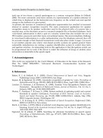
The simulation of

the effect of the controller is shown in Fig.16 as a bode plot. The frequency domain
simulation was done by Matlab v6.5.


Fig. 16. Bode plots of the open loop and closed loop systems under the effect of spatial
∞
H
controller

Active Vibration Control of a Smart Beam by Using a Spatial Approach 401
The vibration attenuation levels at the first two flexural resonance frequencies were found to
be 27.2 dB and 23.1 dB, respectively. The simulated results show that the designed controller
is effective on the suppression of undesired vibration levels.

4.1 Implementation of the Spatial Controller
This section presents the implementation of the spatial
∞
H controller for suppressing the
free and forced vibrations of the smart beam. The closed loop experimental setup is shown
in Fig.17. The displacement of the smart beam at a specific location was measured by using a
Keyence Laser Displacement Sensor (LDS) and converted to a voltage output that was sent
to the SensorTech SS10 controller unit via the connector block. The controller output was
converted to the analog signal and amplified 30 times by SensorTech SA10 high voltage
power amplifier before being applied to the piezoelectric patches. The controller unit is
hosted by a Linux machine on which a shared disk drive is present to store the
input/output data and the C programming language based executable code that is used for
real-time signal processing.

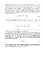
For the free vibration control, the smart beam was given an initial 5 cm tip deflection and
the open loop and closed loop time responses of the smart beam were measured. The results

are presented in Fig.18 which shows that the controlled time response of the smart beam
settles nearly in 1.7 seconds. Hence, the designed controller proves to be very effective on
suppressing the free vibration of the smart beam.


Fig. 17. The closed loop experimental setup
402 New Developments in Robotics, Automation and Control


Fig. 18. Open and closed loop time responses of the smart beam under the effect of spatial
H
∞
controller

The forced vibration control of the smart beam was analyzed in two different
configurations. In the first one, the smart beam was excited for 180 seconds with a shaker
located very close to the root of the smart beam, on which a sinusoidal chirp signal of
amplitude 4.5V was applied. The excitation bandwidth was taken first 5 to 8 Hz and later 40
to 44 Hz to include the first two flexural resonance frequencies separately. The open loop
and closed loop time and frequency responses of the smart beam under respective
excitations are shown in Fig.19-a, Fig.19-b, Fig.20. Note that the Nyquist plot of the nominal
system loop gain under the effect of spatial
∞
H controller given in Fig. 21 shows that the
nominal system is stable.

The experimental attenuation of vibration levels at first two resonance frequencies were
determined from the Bode magnitude plots of the frequency responses of the smart beam
and shown in Fig.20-a and Fig.20-b. The resultant attenuation levels were found as 19.8 dB
and 14.2 dB, respectively. Hence, the experimental results show that the controller is

effective on suppression of the vibration levels. The reason why experimental attenuation
levels are less than the simulated ones is that, the excitation power of the shaker was not
enough to make the smart beam to reach the larger deflections which in turn causes a
smaller magnitude of the open loop time response. The hardware constraints prevent one to
apply higher voltages to the shaker. On the other hand, the magnitude of the experimental
and simulated closed loop frequency responses at resonance frequencies being close to each
other makes one to realize that, the controller works exactly according to the design criteria.
Additionally, one should note that the attenuation levels were obtained from the decibel
Active Vibration Control of a Smart Beam by Using a Spatial Approach 403
magnitudes of the frequency responses. Hence, a simple mathematical manipulation can
give the absolute attenuation levels as a ratio of the maximum time responses of the open
and closed loop systems at the specified resonance frequencies.

In the second configuration, instead of using a sinusoidal chirp signal, constant excitation
was applied for 20 seconds at the resonance frequencies with a mechanical shaker. The open
loop and closed loop time responses of the smart beam were measured and shown in Fig.21
and Fig.22. Although, it is hard to control such a resonant excitation, the time responses
show that the designed controller is still very effective on suppressing the vibration levels.
Recall that the ratio of the maximum time responses of the open and closed loop systems
can be considered as absolute attenuation levels; hence, for this case, the attenuation levels
at each resonance frequency were calculated approximately as 10.4 and 4.17, respectively.

The robustness analysis of the designed controller was performed by Matlab v6.5 μ-
synthesis toolbox. The results are presented in Fig. 23. The theoretical background of μ-
synthesis is detailed in the References (Zhou, 1998 and Ülker, 2003). One should know that
the μ values should be less than unity to accept the controllers to be robust. The Fig.23
shows that the spatial
∞
H controller is robust to the perturbations.

The efficiency of spatial controller in minimizing the overall vibration over the smart beam
was compared by a pointwise controller that is designed to minimize the vibrations only at
point
b
r = 0.99L . For a more detailed description of the pointwise controller design, the
interested reader may refer to the reference (Kırcalı, 2006a and 2006b). However, in order to
give the idea of the previous studies, the comparative effects of the spatial and pointwise
∞
H controllers on suppressing the first two flexural vibrations of the smart beam are briefly
presented in Table 4:


Spatial
∞
H controller Pointwise
∞
H controller
Modes 1
st
mode 2
nd
mode 1
st
mode 2
nd
mode
Simulated attenuation levels
(dB)
27.2 23.1 23.5 24.4
Experimentally obtained

attenuation levels (dB)
19.8 14.2 21.02 21.66
Absolute attenuation levels
under constant resonant
excitation (max. OL time
response/ max. CL time
response)
10.4 4.17 5.75 4.37
Table 4. The comparison of attenuation levels under the effect of spatial and pointwise
∞
H
controllers in forced vibrations
404 New Developments in Robotics, Automation and Control
The simulations show that both controllers work efficiently on suppressing the vibration
levels. The forced vibration control experiments of first configuration show that the
attenuation levels of pointwise controller are slightly higher than those of the spatial one.
Although the difference is not significant especially for the first flexural mode, better
attenuation of pointwise controller would not be a surprise since the respective design
criterion of a pointwise controller is to suppress the undesired vibration level at the specific
measurement point. Additionally, absolute attenuation levels show that under constant
resonant excitation at the first flexural mode, the spatial
∞
H controller has better
performance than the pointwise one. This is because the design criterion of spatial controller
is to suppress the vibration over entire beam; hence, the negative effect of the vibration at
any point over the beam on the rest of the other points is prevented by spatial means. So, the
spatial
∞
H controller resists more robustly to the constant resonant excitation than the
pointwise one.

The implementations of the controllers showed that both controllers reduced the vibration
levels of the smart beam due to its first two flexural modes in comparable efficiency (Kırcalı,
2006a and 2006b). The effect of both controllers on suppressing the first two flexural
vibrations of the smart beam over entire structure can be analyzed by considering the
∞
H
norm of the entire beam. Fig.24 shows the
∞
H norm plots of the smart beam as a function of
r
under the effect of both controllers.


5. General Conclusions

This study presented a different approach in active vibration control of a cantilevered smart
beam.

The required mathematical modeling of the smart beam was conducted by using the
assumed-modes method. This inevitably resulted in a higher order model including a large
number of resonant modes of the beam. This higher order model was truncated to a lower
model by including only the first two flexural vibrational modes of the smart beam. The
possible error due to that model truncation was compensated by employing a model
correction technique which considered the addition of a correction term that consequently
minimized the weighted spatial
2
H norm of the truncation error. Hence, the effect of out-of-
range modes on the dynamics of the system was included by the correction term. During the
modeling phase the effect of piezoelectric patches was also conveniently included in the
model to increase the accuracy of the system model. However, the assumed-modes

modeling alone does not provide any information about the damping of the system. It was
shown that experimental system identification, when used in collaboration with the
analytical model, helps one to obtain more accurate spatial characteristics of the structure.
Since the smart beam is a spatially distributed structure, experimental system identification
based on several measurement locations along the beam results in a number of system
models providing the spatial nature of the beam. Comparison of each experimental and
analytical system models in the frequency domain yields a significant improvement on the
determination of the natural frequencies and helps one to identify the uncertainty on them.
Active Vibration Control of a Smart Beam by Using a Spatial Approach 405
Also, tuning the modal damping ratios until the magnitude of both frequency responses
coincide at resonance frequencies gives valid damping values and the corresponding
uncertainty for each modal damping ratio.

This study also presented the active vibration control of the smart beam. A spatial
∞
H
controller was designed for suppressing the first two flexural vibrations of the smart beam.
The efficiency of the controller was demonstrated both by simulations and experimental
implementation. The effectiveness of spatial controller on suppressing the vibrations of the
smart beam over its entire body was also compared with a pointwise one.


a) Within excitation of 5-8 Hz

b) Within excitation of 40-44 Hz
Fig. 19. Time responses of the smart beam
406 New Developments in Robotics, Automation and Control
Fig. 20. Open and closed loop frequency
responses of the smart beam
Fig. 21. Nyquist plot

Fig. 21. Open and closed loop time responses
at first resonance frequency

Fig. 22. Open and closed loop time
responses at second resonance frequency
Active Vibration Control of a Smart Beam by Using a Spatial Approach 407

6. References

Bai M., Lin G. M., (1996). The Development of DSP-Based Active Small Amplitude Vibration
Control System for Flexible Beams by Using the LQG Algorithms and Intelligent
Materials,
Journal of Sound and Vibration, 198, Vol. 4, pp. 411-427.
Balas G., Young P. M., (1995). Control Design For Variations in Structural Natural
Frequencies,
Journal of Guidance, Control and Dynamics, Vol. 18, No. 2.
Baz A., Poh S., (1988). Performance of an Active Control System with Piezoelectric
Actuators,
Journal of Sound and Vibration, 126(2), pp. 327-343.
Clark R.L., (1997). Accounting for Out-of-Bandwidth Modes in the Assumed Modes
Approach: Implications on Colocated Output Feedback Control,
Transactions of the
ASME, Journal of Dynamic Systems, Measurement, and Control
, Vol. 119, pp. 390-395.
Crawley E.F., Louis J., (1989). Use of Piezoelectric Actuators as Elements of Intelligent
Structures,
AIAA Journal, Vol. 125, No. 10, pp. 1373-1385
Çalışkan T., (2002).
Smart Materials and Their Applications in Aerospace Structures, PhD Thesis,

Middle East Technical University.

Fig. 23. μ-analysis for spatial
∞
H controller

Fig. 24. Simulated
∞
H norm plots of closed
loop systems under the effect of pointwise
and spatial
∞
H controllers