mos 2010 study guide for microsoft phần 5 ppsx
Bạn đang xem bản rút gọn của tài liệu. Xem và tải ngay bản đầy đủ của tài liệu tại đây (1.36 MB, 70 trang )
5 Applying Formulas and Functions 239
1. Select the cell in which you want to place the average.
2. On the Formulas tab, in the Function Library group, click the More Functions
button, point to Statistical, and then in the list, click AVERAGE.
3. In the Function Arguments box, enter the cell range that you want to average,
and then click OK.
➤ To nd the lowest value in a data range
1. Select the cell immediately below or to the right of the values you want to evaluate.
2. On the Formulas tab, in the Function Library group, click the AutoSum arrow, and
then in the list, click Min.
3. Verify that the cell range displayed in the formula is correct, and then press Enter.
Or
1. Select the cell in which you want to place the minimum value.
2. On the Formulas tab, in the Function Library group, click the More Functions
button, point to Statistical, and then in the list, click MIN.
3. In the Function Arguments box, enter the cell range you want to evaluate, and
then click OK.
➤ To nd the highest value in a data range
1. Select the cell immediately below or to the right of the values you want to evaluate.
2. On the Formulas tab, in the Function Library group, click the AutoSum arrow, and
then in the list, click Max.
3. Verify that the cell range displayed in the formula is correct, and then press Enter.
Or
1. Select the cell in which you want to place the maximum value.
2. On the Formulas tab, in the Function Library group, click the More Functions
button, point to Statistical, and then in the list, click MAX.
3. In the Function Arguments box, enter the cell range you want to evaluate, and
then click OK.
240 Exam 77-882 Microsoft Excel 2010
Practice Tasks
The practice les for these tasks are located in the Excel\Objective5 practice le
folder. If you want to save the results of the tasks, save them in the same folder with
My appended to the le name so that you don’t overwrite the original practice le.
●
On the Summary worksheet of the SummaryFormula workbook, do the
following:
❍
In cell B18, create a formula that returns the number of non-empty
cells in the Period range. Then in cell B19, create a formula that returns
the number of empty cells in the same range.
❍
In cell C18, create a formula that returns the average value in the Sales
range.
❍
In cell D5, create a formula that returns the lowest Sales value for the
Fall period.
●
On the Sales By Region worksheet of the Sales workbook, do the following:
❍
Create subtotals of sales amounts rst by Period and then by Region.
❍
Find the average sales by Period and then by Region.
❍
Find the maximum and minimum values by Period and then by Region.
52 Enforce Precedence
A formula can involve multiple types of calculations. Unless you specify another order of
precedence, Excel evaluates formula content and processes calculations in this order:
1 Reference operators The colon (:), space ( ), and comma (,) symbols
2 Negation The negative (–) symbol in phrases such as –1
3 Percentage The percent (%) symbol
4 Exponentiation The raising to a power (^) symbol
5 Multiplication and division The multiply (*) and divide (/) symbols
6 Addition and subtraction The plus (+) and minus (-) symbols
7 Concatenation The and (&) symbol connecting two strings of text
8 Comparison The equal (=), less than (<), and greater than (>) symbols and any
combination thereof
5 Applying Formulas and Functions 241
If multiple calculations within a formula have the same precedence, Excel processes them
in order from left to right.
You can change the order in which Excel processes the calculations within a formula
by enclosing the calculations you want to perform rst in parentheses. Similarly, when
you use multiple calculations to represent one value in a formula, you can enclose the
calculations in parentheses to instruct Excel to process the calculations as a unit before
incorporating the results of the calculation in the formula.
The following table illustrates the effect of changing precedence within a simple formula.
Formula Result
=1+2-3+4-5+6 5
=(1+2)-(3+4)-(5+6) –15
=1+(2-3)+4-(5+6) –7
➤ To change the order of calculation within a formula
➜ Enclose the calculations you want to perform rst within parentheses.
Practice Tasks
There are no practice les for these tasks. Simply open a blank workbook.
●
In cell A1 of a worksheet, enter the following formula:
=5x2+7-12
●
Copy the formula from cell A1 to cells A2:A5. Edit each of the copied formulas,
placing parentheses around different groupings to view the effect.
242 Exam 77-882 Microsoft Excel 2010
53 Apply Cell References in Formulas
Formulas in an Excel worksheet most often involve functions performed on the values
contained in one or more other cells on the worksheet (or on another worksheet). A ref-
erence that you make in a formula to the contents of a worksheet cell is either a relative
reference, an absolute reference, or a mixed reference. A relative reference changes in
relation to the cell in which the referring formula is originally entered; an absolute refer-
ence doesn’t change. It is important to understand the difference and to know which to
use when creating a formula.
A relative reference to a cell takes the form A1. When you copy or ll a formula from
the original cell to other cells, a relative reference changes to indicate the cell having the
same relationship to the formula cell that A1 did to the original formula cell. For example,
copying a formula that refers to cell A1 one row down changes the A1 reference to A2;
copying the formula one column to the right changes the A1 reference to B1.
An absolute reference takes the form $A$1; the dollar sign indicates an absolute reference
to column A and an absolute reference to row 1. When you copy or ll a formula from the
original cell to other cells, an absolute reference does not change—regardless of the re-
lationship to the referenced cell, the reference stays the same.
A mixed reference refers absolutely to one part of the reference and relatively to the other.
The mixed reference A$1 always refers to row 1, and $A1 always refers to column A.
5 Applying Formulas and Functions 243
You can reference cells in other worksheets of your workbook. For example, you might
prepare a Summary worksheet that displays results based on data tracked on other work-
sheets. References to cells on other worksheets can be relative, absolute, or mixed.
Tip You can reference a worksheet by whatever name appears on the worksheet tab
You can reference cells in other workbooks. For example, you might prepare a report
that collates data from workbooks submitted by multiple regional managers.
When referencing a workbook located in a folder other than the one your active work-
book is in, enter the path to the le along with the le name. If the path includes a
non-alphabetical character (such as the backslash in “C:\”), enclose the path in single
quotation marks.
➤ To relatively reference the contents of a cell
➜ Enter the column letter followed by the row number, like this:
A1
➤ To absolutely reference the contents of a cell
➜ Precede the column letter and row number with dollar signs, like this:
$A$1
➤ To absolutely reference a column or row
➜ Precede the column letter or row number with a dollar sign.
➤ To reference a cell on a different worksheet in the same workbook
➜ Enter the worksheet name and cell reference, separated by an exclamation point,
like this:
Data!C2
Or
1. With the cursor positioned where you want to insert the reference, click the tab of
the worksheet containing the cell you want to reference.
2. Click the cell or select the cell range you want to reference, and then press Enter to
enter the cell reference into the formula and return to the original worksheet.
244 Exam 77-882 Microsoft Excel 2010
➤ To reference a cell in another workbook in the same folder
➜ Enter the workbook name in square brackets followed by the worksheet name and
cell reference, separated by an exclamation point, like this:
[Sales.xlsx]Data!C2
➜ Enter the path to the workbook, followed the workbook name in square brackets,
followed by the worksheet name, enclosing everything in single quotes, Then enter
an exclamation point followed by the cell reference, like this:
='C:\PROJECTS\MOS2010\Excel Files\[test.xlsx]Sheet1'!$A$1
Or
1. Open the workbook that contains the cell you want to reference, and then switch
to the workbook you want to create the formula in.
2. With the cursor positioned where you want to insert the reference, switch to the
second workbook, click the tab of the worksheet containing the cell you want
to reference, click the cell or select the range you want to reference, and then
press Enter.
Practice Tasks
The practice les for these tasks are located in the Excel\Objective5 practice le
folder. If you want to save the results of the tasks, save them in the same folder with
My appended to the le name so that you don’t overwrite the original practice le.
●
In the MultiplicationTable workbook, on the Practice worksheet, create a for-
mula in cells B2:T20 to complete the multiplication table of the numbers 1
through 20. (Challenge: Create the table in six or fewer steps.) Compare the
formulas in your multiplication table with those on the Results worksheet.
●
In the SalesBySeason workbook, on the Summary worksheet, display the
total sales for each period in cells B2:B5 by referencing the corresponding
worksheets.
5 Applying Formulas and Functions 245
54 Apply Conditional Logic in Formulas
Creating Conditional Formulas
You can use a formula to display specic results when certain conditions are met. To do
so, you create a formula that uses the conditional logic provided by the IF() function
or one of its variations. A basic formula that uses the IF() function performs a logical test
and then returns one of two results based on whether the logical test evaluates as TRUE
or FALSE.
The correct syntax for the IF() function is as follows:
=IF(logical_test,value_if_true,value_if_false)
Tip The IF() function in Excel is equivalent to an IF…THEN…ELSE function in a computer
program
The logical test and the result can include text strings or calculations. Enclose text strings
within the formula in quotation marks. Do not enclose numeric values or calculations in
quotation marks.
Excel 2010 includes the additional conditional logic functions shown in the following table.
Function Description
AVERAGEIF()
AVERAGEIFS()
Returns the average of values in a range that meet one or more criteria
COUNTIF()
COUNTIFS()
Returns the number of cells in a range that meet one or more criteria
SUMIF()
SUMIFS()
Returns the sum of values in a range that meet one or more criteria
IFERROR() Returns one value if a formula results in an error and another if it doesn’t
Strategy Experiment with each of the conditional functions Follow the prompts given
in the tooltip that appears when you begin entering the formula to be sure you provide
valid arguments for each function
246 Exam 77-882 Microsoft Excel 2010
Nesting Functions
You can nest additional functions within an IF() function so that Excel evaluates multiple
conditions before returning a result. You can use nested functions to do the following:
● Perform a calculation that results in an argument used by the IF() function, like this:
=IF(SUM(D1:D8)>=80,”Congratulations, you passed!”,”Sorry, you failed. Please try
again.”)
● Combine multiple logical tests, like this:
=IF(AND(Year=2011,Month=”July”),B2*C4,”No”)
You can add logical tests to a conditional formula by using the following functions:
●
AND() Returns a value of TRUE only if every logical test within it is TRUE.
●
OR() Returns a value of TRUE if any logical test within it is TRUE.
●
NOT() Reverses the logical outcome of a logical test, so if the test is TRUE, NOT
returns FALSE. For example, NOT(A1=3), returns TRUE as long as the value in cell
A1 is not equal to 3. You use this function when you want to check whether a
cell is not equal to a certain value.
You place the AND(), OR(), and NOT() functions before the associated arguments.
➤ To use a single conditional logic argument in a formula
➜ Enter the function followed by a parenthetical phrase containing the logical test(s),
the result if the condition is true, and the result if the condition is false, separated
by commas, like this:
=IF(A3<>"",A3+B3,B3+C3)
➤ To use a series of conditional logic arguments in a formula
➜ Nest one or more additional functions within the IF() function, like this:
=IF(OR(Month="June",Month="July",Month="August"),"See you next school
year!","Enjoy the school year!")
5 Applying Formulas and Functions 247
Practice Tasks
The practice le for these tasks is located in the Excel\Objective5 practice le folder.
If you want to save the results of the tasks, save them in the same folder with My
appended to the le name so that you don’t overwrite the original practice le.
●
On the Expense Statement worksheet of the ConditionalFormula workbook,
do the following:
❍
In cell C25, use the AND() function to determine whether the Entertainment
total is less than $200.00 and the Misc. total is less than $100.00.
❍
In cell C26, use the OR() function to determine whether the Entertainment
total is more than $200.00 or the Misc. total is more than $100.00.
❍
In cell C27, use the IF() function to display the text "Expenses are okay"
if the function in C25 evaluates to TRUE and "Expenses are too high" if it
evaluates to FALSE.
❍
In cell C28, use the IF() function to display the text "Expenses are okay" if
the function in C26 evaluates to NOT TRUE and "Expenses are too high"
if it evaluates to NOT FALSE.
❍
Add 60.00 to either the Entertainment column or the Misc. column to
check your work.
55 Apply Named Ranges in Formulas
To simplify the process of creating formulas that refer to a specic range of data, and to
make your formulas easier to create and read, you can refer to a cell or range of cells by
a name that you dene. For example, you might name a cell containing an interest rate
Interest, or a range of cells containing nonwork days Holidays. In a formula, you can refer
to a named range by name. Thus a formula might look like this:
=WORKDAY(StartDate,WorkingDays,Holidays)
A formula that uses named ranges is easier to understand than one that uses standard
references, which might look like this:
=WORKDAY(B2,B$3,Data!B2:B16)
248 Exam 77-882 Microsoft Excel 2010
Each named range has a scope, which is the context in which the name is recognized. The
scope can be the entire workbook or a specic worksheet. The workbook scope allows you
to use the same name on multiple worksheets. You can include a comment with each
name to provide more information about the range. (The comment is visible only in the
Name Manager.)
After dening a named range, you can change the name or the cells included in the
named range. You can delete a named range denition from the Name Manager.
Note that deleting a cell from a worksheet does not delete any associated named
range. Invalid named ranges are indicated in the Name Manager by #REF! in the
Value column.
➤ To dene a selected cell or range of cells as a named range
➜ In the Name box at the right end of the Formula Bar, enter the name, and then
press Enter.
Or
1. On the Formulas tab, in the Dened Names group, click the Dene Name button.
2. In the New Name dialog box, enter the name in the Name box.
Tip The New Name dialog box does not indicate whether the selected cell or cells are
already part of an existing named range
3. In the Scope list, click Workbook to dene the named range for the entire workbook,
or click a specic worksheet name.
5 Applying Formulas and Functions 249
4. In the Comment box, enter any notes you want to make for your own reference.
5. Verify that the cell or range of cells in the Refers to box is correct, and then click OK.
Tip If a cell is part of multiple named ranges, only the rst name is shown in the Name
box The Name box displays the name of a multiple-cell named range only when all cells
in the range are selected
➤ To redene the cells in a named range
1. On the Formulas tab, in the Dened Names group, click the Name Manager button.
2. In the Name Manager window, click the named range you want to change, and then
click Edit.
3. In the Edit Name dialog box, do one of the following, and then click OK.
❍
In the Refers to box, enter the cell range to which you want the name to refer.
❍
If necessary, click the Minimize button at the right end of the Refers to box
to expose the worksheet area. Then on the worksheet, drag to select the cells
that you want to include in the named range.
➤ To change the name of the cells in a named range
1. On the Formulas tab, in the Dened Names group, click the Name Manager button.
2. In the Name Manager window, click the named range you want to change, and then
click Edit.
3. In the Edit Name dialog box, change the name in the Name box, and then click OK.
➤ To delete a named range denition
1. On the Formulas tab, in the Dened Names group, click the Name Manager button.
2. In the Name Manager window, click the named range you want to delete, and click
Delete. Then click OK to conrm the deletion.
Practice Tasks
The practice le for these tasks is located in the Excel\Objective5 practice le folder.
If you want to save the results of the tasks, save them in the same folder with My
appended to the le name so that you don’t overwrite the original practice le.
●
In the MultiplicationTable workbook, on the Results worksheet, dene cells A1:T1
as a range named FirstRow, and cells A1:A20 as a range named ColumnA. Then
change the formulas in cells B2:T20 to reference the named ranges.
250 Exam 77-882 Microsoft Excel 2010
56 Apply Cell Ranges in Formulas
You can refer to the content of a range of adjacent cells. For example, you might use a
formula to add the values of a range of cells, or to nd the maximum value in all the
cells in a row. When referencing a range of cells in a formula, the cell references can
be relative, absolute, or mixed.
➤ To relatively reference the contents of a range of cells
➜ Enter the upper-left cell of the range and the lower-right cell of the range, separated
by a colon, like this:
A1:B3
➤ To enter a relative reference to a range of cells in a formula
1. Position the cursor where you want to insert the cell range reference.
2. Drag to select the cell range and insert the cell range reference.
➤ To absolutely reference the contents of a range of cells
➜ Enter the absolute reference of the upper-left cell of the range and the absolute
reference of the lower-right cell of the range, separated by a colon, like this:
$A$1:$B$3
5 Applying Formulas and Functions 251
Practice Tasks
The practice le for these tasks is located in the Excel\Objective5 practice le folder.
If you want to save the results of the tasks, save them in the same folder with My
appended to the le name so that you don’t overwrite the original practice le.
●
On the Product Sales worksheet of the CellRange workbook, in cells C95,
C101, and C104, calculate the sales total for each category by using a relative
cell range reference.
●
In cell C86 of the Product Sales worksheet, calculate the Cacti sales total by
using an absolute cell range reference.
Objective Review
Before nishing this chapter, ensure that you have mastered the following skills:
5.1 Create Formulas
5.2 Enforce Precedence
5.3 Apply Cell References in Formulas
5.4 Apply Conditional Logic in Formulas
5.5 Apply Named Ranges in Formulas
5.6 Apply Cell Ranges in Formulas
253
6 Presenting Data
Visually
The skills tested in this section of the Microsoft Ofce Specialist exam for Microsoft
Excel 2010 relate to adding visual interest to a worksheet. Specically, the following
objectives are associated with this set of skills:
6.1 Create Charts Based on Worksheet Data
6.2 Apply and Manipulate Illustrations
6.3 Create and Modify Images
6.4 Apply Sparklines
You can insert many of the same graphic elements in an Excel workbook that you can
insert in other Microsoft Ofce documents, including clip art, SmartArt diagrams, shapes,
screenshots, and pictures. You can also express numeric data by creating charts, and
summarize numeric data by using sparklines.
This chapter guides you in studying ways of inserting and modifying charts, graphics
images, and sparklines.
Practice Files Before you can complete the practice tasks in this chapter, you need
to copy the book’s practice les to your computer The practice les you’ll use to complete
the tasks in this chapter are in the Excel\Objective6 practice le folder A complete list
of practice les is provided in “Using the Book’s Companion Content”at the beginning of
this book
Contents
6 Presenting Data
Visually 253
6.1. . . . . . . . . . . . . . . . . . . . . . . . . . . . . . . . . . . . Create Charts Based on Worksheet Data
254
Plotting Charts . . . . . . . . . . . . . . . . . . . . . . . . . . . . . . . . . . . . . . . . . . . . . . . . . . . . .254
Applying Layouts and Styles . . . . . . . . . . . . . . . . . . . . . . . . . . . . . . . . . . . . . . . . .257
Moving and Sizing Charts . . . . . . . . . . . . . . . . . . . . . . . . . . . . . . . . . . . . . . . . . . .258
Editing Data . . . . . . . . . . . . . . . . . . . . . . . . . . . . . . . . . . . . . . . . . . . . . . . . . . . . . . .259
Conguring Chart Elements. . . . . . . . . . . . . . . . . . . . . . . . . . . . . . . . . . . . . . . . . .260
Practice Tasks . . . . . . . . . . . . . . . . . . . . . . . . . . . . . . . . . . . . . . . . . . . . . . . . . . . . . .263
6.2 . . . . . . . . . . . . . . . . . . . . . . . . . . . . . . . . . . . . . . . . Apply and Manipulate Illustrations
264
Inserting and Formatting Clip Art. . . . . . . . . . . . . . . . . . . . . . . . . . . . . . . . . . . . .264
Inserting and Modifying SmartArt Diagrams . . . . . . . . . . . . . . . . . . . . . . . . . . .265
Inserting and Formatting Shapes . . . . . . . . . . . . . . . . . . . . . . . . . . . . . . . . . . . . .267
Capturing Screenshots . . . . . . . . . . . . . . . . . . . . . . . . . . . . . . . . . . . . . . . . . . . . . .269
Practice Tasks . . . . . . . . . . . . . . . . . . . . . . . . . . . . . . . . . . . . . . . . . . . . . . . . . . . . . .270
6.3 . . . . . . . . . . . . . . . . . . . . . . . . . . . . . . . . . . . . . . . . . . . . . . . Create and Modify Images
271
Practice Tasks . . . . . . . . . . . . . . . . . . . . . . . . . . . . . . . . . . . . . . . . . . . . . . . . . . . . . .273
6.4. . . . . . . . . . . . . . . . . . . . . . . . . . . . . . . . . . . . . . . . . . . . . . . . . . . . . . . . . Apply Sparklines
273
Practice Tasks . . . . . . . . . . . . . . . . . . . . . . . . . . . . . . . . . . . . . . . . . . . . . . . . . . . . . .275
Objective Review . . . . . . . . . . . . . . . . . . . . . . . . . . . . . . . . . . . . . . . . . . . . . . . . . . . . . . . .276
254 Exam 77-882 Microsoft Excel 2010
61 Create Charts Based on Worksheet Data
Plotting Charts
Charts are an important tool for data analysis and are therefore a common component
of certain types of worksheets. You can easily plot selected data as a chart to make it
easy to identify trends and relationships that might not be obvious from the data itself.
Tip You must select only the data you want to appear in the chart If the data is not in a
contiguous range of rows or columns, either rearrange the data or hold down the Ctrl key
while you select noncontiguous ranges
Different types of data are best suited for different types of charts. The following table
shows the available chart types and the type of data they are particularly useful for plotting.
Chart type Typically used to show
Column Variations in value over time or comparisons
Line Multiple data trends over evenly spaced intervals
Pie Percentages assigned to different components of a single item (non-negative,
non-zero, no more than seven values)
Bar Variations in value over time or the comparative values of several items at a
single point in time
Area Multiple data series as cumulative layers showing change over time
X Y (Scatter) Correlations between independent items
Stock Stock market or similar activity
Surface Trends in values across two different dimensions in a continuous curve,
such as a topographic map
Doughnut Percentages assigned to different components of more than one item
Bubble Correlations between three or more independent items
Radar Percentages assigned to different components of an item, radiating from a
center point
6 Presenting Data Visually 255
To plot selected data as a chart, all you have to do is specify the chart type. If the type of
chart you initially selected doesn’t adequately depict your data, you can change the type
at any time. The 11 chart types each have several two-dimensional and three-dimensional
variations, and you can customize each aspect of each variation.
When you plot worksheet data, a row or column of values, which in the charting world
are called data points, constitutes a set of data called a data series. Each data point in a
data series is represented graphically in the chart by a data marker and in the chart legend
by a unique color or pattern. The data is plotted against an x-axis (or category axis) and a
y-axis (or value axis). Three-dimensional charts also have a z-axis (or series axis). Sometimes
a chart does not produce the results you expect because the data series are plotted against
the wrong axes; that is, Excel is plotting the data by row when it should be plotting by
column, or vice versa. You can quickly switch the rows and columns to see whether that
produces the desired effect. To see what Excel is doing behind the scenes, you can open
the Select Data Source dialog box, which shows you exactly what is plotted where.
256 Exam 77-882 Microsoft Excel 2010
Strategy Practice plotting the same data in different ways In particular, understand
the effects of plotting data by column or by row
➤ To plot selected data as a chart on the worksheet
Tip Before plotting the data, ensure that it is correctly set up for the type of chart you
want to create For example, a pie chart can display only one data series
➜
On the Insert tab, in the Charts group, click the button of the chart type you want,
and then click a sub-type.
➤ To change the type of a selected chart
1. On the Chart Tools Design contextual tab, in the Type group, click the Change Chart
Type button.
2. In the Change Chart Type dialog box, click a new type and sub-type, and then click OK.
➤ To switch rows and columns in a selected chart
➜ On the Design contextual tab, in the Data group, click the Switch Row/Column
button.
Or
6 Presenting Data Visually 257
1. On the Design contextual tab, in the Data group, click the Select Data button.
Or
Right-click the chart border or data area, and then click Select Data.
2. In the Select Data Source dialog box, click Switch Row/Column, and then click OK.
Applying Layouts and Styles
You can apply predened combinations of layouts and styles to quickly format a chart. You
can also apply a shape style to the chart area to set it off from the rest of the sheet.
➤ To change the layout of a selected chart
➜ On the Chart Tools Design contextual tab, in the Chart Layouts gallery, click the
layout you want.
➤ To apply a style to a selected chart
➜ On the Design contextual tab, in the Chart Styles gallery, click the style you want.
➤ To apply a shape style to a selected chart
➜ On the Chart Tools Format contextual tab, in the Shape Styles gallery, click the
style you want.
258 Exam 77-882 Microsoft Excel 2010
Moving and Sizing Charts
The charts you create often don’t appear where you want them on a worksheet, and they
are often too big or too small to adequately show their data. You can move and size a
chart by using simple dragging techniques.
If you prefer to display a chart on its own sheet instead of embedding it in the work-
sheet containing its data, you can easily move it. You can also move it to any other
existing worksheet in the workbook.
➤ To move a selected chart to a chart sheet
1. On the Chart Tools Design contextual tab, in the Location group, click the Move
Chart button.
Or
Right-click the chart border, and then click Move Chart.
2. In the Move Chart dialog box, click New sheet, and then if you want, enter a
name for the sheet.
3. Click OK.
➤ To move a selected chart to a different sheet in the same workbook
1. Open the Move Chart dialog box, click Object in, and then select the worksheet
you want from the list.
2. Click OK.
➤ To change the size of a selected chart
➜ Point to a handle (set of dots) on the chart's frame, and drag in the direction you
want the chart to grow or shrink.
➜ Point to a handle in a corner of the chart's frame, hold down the Shift key, and
drag in the direction you want the chart to grow or shrink proportionally.
6 Presenting Data Visually 259
➜ On the Chart Tools Format contextual tab, in the Size group, change the Shape
Height and Shape Width settings.
Or
1. On the Format contextual tab, click the Size dialog box launcher.
2. In the Size and Properties dialog box, change the settings in the Size and rotate or
Scale area, and then click Close.
Tip Select the Lock Aspect Ratio check box before changing the settings if you want
to size the chart proportionally
Editing Data
A chart is linked to its worksheet data, so any changes you make to the plotted data are
immediately reected in the chart. If you add or delete values in a data series or add or
remove an entire series, you need to increase or decrease the range of the plotted data in
the worksheet.
➤ To edit the data in a chart
➜ In the linked Excel worksheet, change the plotted values.
➤ To change the range of plotted data in a selected chart
➜ In the linked Excel worksheet, drag the corner handles of the series selectors until
they enclose the series you want to plot.
260 Exam 77-882 Microsoft Excel 2010
Conguring Chart Elements
To augment the usefulness or the attractiveness of a chart, you can add elements such
as a title, axis labels, data labels, a data table, and gridlines. You can adjust each element,
as well as the plot area (the area dened by the axes) and the chart area (the entire chart
object), in appropriate ways.
Strategy You can tailor the elements of charts in too many ways for us to cover them in
detail here In addition to choosing options from galleries, you can open a Format dialog
box for each type of element Make sure you are familiar with the chart elements and how
to use them to enhance a chart
➤ To add a chart title
1. On the Chart Tools Layout contextual tab, in the Labels group, click the Chart Title
button.
2. In the Title gallery, click the option you want.
3. Select the placeholder title, and replace it with the one you want.
6 Presenting Data Visually 261
➤ To add or remove axis titles
1. On the Layout contextual tab, in the Labels group, click the Axis Titles button.
2. In the list, point to Primary Horizontal Axis Title, and then click None or Title Below
Axis; or click More Primary Horizontal Axis Title Options, make specic selections in
the Format Axis Title dialog box, and then click Close.
Or
In the list, point to Primary Vertical Axis Title, and then click None, Rotated Title,
Vertical Title, or Horizontal Title; or click More Primary Vertical Axis Title Options,
make specic selections in the Format Axis Title dialog box, and then click Close.
3. Select the placeholder axis title, and enter the text you want to appear as the
axis title.
➤ To add, remove, or move the legend
1. On the Layout contextual tab, in the Labels group, click the Legend button.
2. In the Legend gallery, click the Show Legend (Right, Top, Left, or Bottom) or
Overlay Legend (Right or Left) option you want.
Or
Click More Legend Options, make specic selections in the Format Legend dialog
box, and then click Close.
➤ To display data labels
1. On the Layout contextual tab, in the Labels group, click the Data Labels button.
2. In the Data Labels gallery, click Show to display the value of each data point on
its marker.
Or
In the Data Labels gallery, click More Data Label Options, make specic selections
(including the number format and decimal places) in the Format Legend dialog box,
and then click Close.
Tip Data labels can clutter up all but the simplest charts If you need to show the data
for a chart on a separate chart sheet, consider using a data table instead
Download from Wow! e B o o k < w w w . w owebook.com>
262 Exam 77-882 Microsoft Excel 2010
➤ To display the chart data under the axis titles
1. On the Layout contextual tab, in the Labels group, click the Data Table button.
2. In the Data Table gallery, click Show Data Table or Show Data Table with
Legend Keys.
Or
Click More Data Table Options, make specic selections in the Format Data Table
dialog box, and then click Close.
➤ To display or hide axes
1. On the Layout contextual tab, in the Axes group, click the Axes button.
2. In the list, point to Primary Horizontal Axis and then click None, Show Left to Right
Axis, Show Axis without labeling, or Show Right to Left Axis; or click More Primary
Horizontal Axis Options, make specic selections in the Format Axis dialog box, and
then click Close.
Or
In the list, point to Primary Vertical Axis and then click None, Show Default Axis,
Show Axis in Thousands, Show Axis in Millions, Show Axis in Billions, or Show
Axis with Log Scale; or click More Primary Vertical Axis Options, make specic
selections in the Format Axis dialog box, and then click Close.
➤ To display or hide gridlines
1. On the Layout contextual tab, in the Axes group, click the Gridlines button.
2. In the Gridlines list, point to Primary Horizontal Gridlines and then click None,
Major Gridlines, Minor Gridlines, or Major & Minor Gridlines; or click More
Primary Horizontal Gridlines Options, make specic selections in the Format
Major Gridlines dialog box, and then click Close.
Or
In the Gridlines list, point to Primary Vertical Gridlines and then click None, Major
Gridlines, Minor Gridlines, or Major & Minor Gridlines; or click More Primary
Vertical Gridlines Options, make specic selections in the Format Major Gridlines
dialog box, and then click Close.
6 Presenting Data Visually 263
➤ To select a chart element for formatting
➜ On the Layout contextual tab, in the Current Selection group, click the element
you want in the Chart Elements list, and then click the Format Selection button
to open the corresponding Format dialog box.
Tip Only those elements that are present in the chart appear in the Chart Elements list
Practice Tasks
The practice les for these tasks are located in the Excel\Objective6 practice le
folder. If you want to save the results of the tasks, save them in the same folder with
My appended to the le name so that you don’t overwrite the original practice le.
●
In the DataSource workbook, use the data on the Seattle worksheet to plot a
simple pie chart.
●
In the Plotting workbook, on the Sales worksheet, plot the data as a simple
2-D column chart. Then switch the rows and columns.
●
In the Plotting workbook, on the Sales worksheet, change the chart to a 3-D
Clustered Column chart. Then apply Layout 1, Style 34, and the Subtle Effect –
Accent 3 shape style.
●
In the SizingMoving workbook, on the Sales worksheet, increase the size of
the chart until it occupies cells A1:L23. Then move it to a new chart sheet
named Sales Chart.
●
In the Editing workbook, on the Sales worksheet, change the October sales
amount for the Flowers category to 888.25. Then add the November data
series to the chart, and change the way the data is plotted so that you can
compare sales for the two months.
●
In the ChartElements workbook, on the Seattle worksheet, add the title Air
Quality Index Report to the chart. Then add data labels that show the percent-
age relationship of each data marker to the whole, with no decimal places.