Mechanics.Of.Materials.Saouma Episode 8 potx

Draft
9.2 Airy Stress Functions; Plane Strain 3
13 On the face x
1
= L, we have a unit normal n = e
1
and a surface traction
t = Te
1
= T
21
e
2
+ T
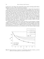
31
e
3
(9.9)
this distribution of surface traction on the end face gives rise to the following resultants
R
1
=

T
11
dA = 0 (9.10-a)
R
2
=

T

21
dA = µθ


x
3
dA = 0 (9.10-b)
R
3
=

T
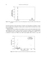
31
dA = µθ


x
2
dA = 0 (9.10-c)
M
1
=

(x
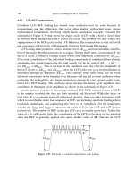
2
T
31
− x
3
T

21
)dA = µθ


(x
2
2
+ x
2
3
)dA = µθ

J (9.10-d)
M
2
= M
3
= 0 (9.10-e)
We note that

(x
2
2
+ x
3
3
)
2
dA is the polar moment of inertia of the cross section and is equal to
J = πa

4
/2, and we also note that

x
2
dA =

x
3
dA = 0 because the area is symmetric with respect to
the axes.
14 From the last equation we note that
θ

=
M
µJ
(9.11)
which implies that the shear modulus µ can be determined froma simple torsion experiment.
15 Finally, in terms of the twisting couple M, the stress tensor becomes
[T]=


0 −
Mx
3
J
Mx
2
J

−
Mx
3
J
00
Mx
2
J
00


(9.12)
9.2 Airy Stress Functions; Plane Strain
16 If the deformation of a cylindrical body is such that there is no axial components of the displacement
and that the other components do not depend on the axial coordinate, then the body is said to be in a
state of plane strain. If e
3
is the direction corresponding to the cylindrical axis, then we have
u
1
= u
1
(x
1
,x
2
),u
2
= u
2

(x
1
,x
2
),u
3
= 0 (9.13)
and the strain components corresponding to those displacements are
E
11
=
∂u
1
∂x
1
(9.14-a)
E
22
=
∂u
2
∂x
2
(9.14-b)
E
12
=
1
2


∂u
1
∂x
2
+
∂u
2
∂x
1

(9.14-c)
E
13
= E
23
= E
33
= 0 (9.14-d)
and the non-zero stress components are T
11
,T
12
,T
22
,T
33
where
T
33
= ν(T

11
+ T
22
) (9.15)
Victor Saouma Mechanics of Materials II
Draft
4 SOME ELASTICITY PROBLEMS
17 Considering a static stress field with no body forces, the equilibrium equations reduce to:
∂T
11
∂x
1
+
∂T
12
∂x
2
= 0 (9.16-a)
∂T
12
∂x
1
+
∂T
22
∂x
2
= 0 (9.16-b)
∂T
33

∂x
1
= 0 (9.16-c)
we note that since T
33
= T
33
(x
1
,x
2
), the last equation is always satisfied.
18 Hence, it can be easily verified that for any arbitrary scalar variable Φ, if we compute the stress
components from
T
11
=
∂
2
Φ
∂x
2
2
(9.17)
T
22
=
∂
2
Φ

∂x
2
1
(9.18)
T
12
= −
∂
2
Φ
∂x
1
∂x
2
(9.19)
then the first two equations of equilibrium are automatically satisfied. This function Φ is called Airy
stress function.
19 However, if stress components determined this way are statically admissible (i.e. they satisfy
equilibrium), they are not necessarily kinematically admissible (i.e. satisfy compatibility equations).
20 To ensure compatibility of the strain components, we express the strains components in terms of Φ
from Hooke’s law, Eq. 7.36 and Eq. 9.15.
E
11
=
1
E

(1 − ν
2
)T

11
− ν(1 + ν)T
22

=
1
E

(1 − ν
2
)
∂
2
Φ
∂x
2
2
− ν(1 + ν)
∂
2
Φ
∂x
2
1

(9.20-a)
E
22
=
1

E

(1 − ν
2
)T
22
− ν(1 + ν)T
11

=
1
E

(1 − ν
2
)
∂
2
Φ
∂x
2
1
− ν(1 + ν)
∂
2
Φ
∂x
2
2


(9.20-b)
E
12
=
1
E
(1 + ν)T
12
= −
1
E
(1 + ν)
∂
2
Φ
∂x
1
∂x
2
(9.20-c)
For plane strain problems, the only compatibility equation, 4.140, that is not automatically satisfied is
∂
2
E
11
∂x
2
2
+
∂

2
E
22
∂x
2
1
=2
∂
2
E
12
∂x
1
∂x
2
(9.21)
substituting,
(1 − ν)

∂
4
Φ
∂x
4
1
+2
∂
4
Φ
∂x

2
1
∂x
2
2
+
∂
4
Φ
∂x
4
1

= 0 (9.22)
or
∂
4
Φ
∂x
4
1
+2
∂
4
Φ
∂x
2
1
∂x
2

2
+
∂
4
Φ
∂x
4
2
=0 or ∇
4
Φ=0
(9.23)
Hence, any function which satisfies the preceding equation will satisfy both equilibrium, kinematic,
stress-strain (albeit plane strain) and is thus an acceptable elasticity solution.
21 †We can also obtain from the Hooke’s law, the compatibility equation 9.21, and the equilibrium
equations the following

∂
2
∂x
2
1
+
∂
2
∂x
2
2

(T

11
+ T
22
)=0 or ∇
2
(T
11
+ T
22
)=0
(9.24)
Victor Saouma Mechanics of Materials II
Draft
9.2 Airy Stress Functions; Plane Strain 5
22 †Any polynomial of degree three or less in x and y satisfies the biharmonic equation (Eq. 9.23). A
systematic way of selecting coefficients begins with
Φ=
∞

m=0
∞

n=0
C
mn
x
m
y
n
(9.25)

23 †The stresses will be given by
T
xx
=
∞

m=0
∞

n=2
n(n − 1)C
mn
x
m
y
n−2
(9.26-a)
T
yy
=
∞

m=2
∞

n=0
m(m − 1)C
mn
x
m−1

y
n
(9.26-b)
T
xy
= −
∞

m=1
∞

n=1
mnC
mn
x
m−1
y
n−1
(9.26-c)
24 †Substituting into Eq. 9.23 and regrouping we obtain
∞

m=2
∞

n=2
[(m+2)(m+1)m(m−1)C
m+2,n−2
+2m(m−1)n(n−1)C
mn

+(n+2)(n+1)n(n−1)C
m−2,n+2
]x
m−2
y
n−2
=0
(9.27)
but since the equation must be identically satisfied for all x and y, the term in bracket must be equal to
zero.
(m+2)(m+1)m(m−1)C
m+2,n−2
+2m(m−1)n(n−1)C
mn
+(n+2)(n+1)n(n−1)C
m−2,n+2
= 0 (9.28)
Hence, the recursion relation establishes relationships among groups of three alternate coefficients which
can be selected from












00C
02
C
03
C
04
C
05
C
06
···
0 C
11
C
12
C
13
C
14
C
15
···
C
20
C
21
C
22
C
23

C
24
···
C
30
C
31
C
32
C
33
···
C
40
C
41
C
42
···
C50 C
51
···
C
60
···












(9.29)
For example if we consider m = n = 2, then
(4)(3)(2)(1)C
40
+ (2)(2)(1)(2)(1)C
22
+ (4)(3)(2)(1)C
04
= 0 (9.30)
or 3C
40
+ C
22
+3C
04
=0
9.2.1 Example: Cantilever Beam
25 We consider the homogeneous fourth-degree polynomial
Φ
4
= C
40
x
4

+ C
31
x
3
y + C
22
x
2
y
2
+ C
13
xy
3
+ C
04
y
4
(9.31)
with 3C
40
+ C
22
+3C
04
=0,
26 The stresses are obtained from Eq. 9.26-a-9.26-c
T
xx
=2C

22
x
2
+6C
13
xy +12C
04
y
2
(9.32-a)
T
yy
=12C
40
x
2
+6C
31
xy +2C
22
y
2
(9.32-b)
T
xy
= −3C
31
x
2
− 4C

22
xy −3C
13
y
2
(9.32-c)
Victor Saouma Mechanics of Materials II
Draft
6 SOME ELASTICITY PROBLEMS
These can be used for the end-loaded cantilever beam with width b along the z axis, depth 2a and
length L.
27 If all coefficients except C
13
are taken to be zero, then
T
xx
=6C
13
xy (9.33-a)
T
yy
= 0 (9.33-b)
T
xy
= −3C
13
y
2
(9.33-c)
28 This will give a parabolic shear traction on the loaded end (correct), but also a uniform shear traction

T
xy
= −3C
13
a
2
on top and bottom. These can be removed by superposing uniform shear stress T
xy
=
+3C
13
a
2
corresponding to Φ
2
= −3C
13
a
2
  
C
11
xy.Thus
T
xy
=3C
13
(a
2
− y

2
) (9.34)
note that C
20
= C
02
=0,andC
11
= −3C
13
a
2
.
29 The constant C
13
is determined by requiring that
P = b

a
−a
−T
xy
dy = −3bC
13

a
−a
(a
2
− y

2
)dy (9.35)
hence
C
13
= −
P
4a
3
b
(9.36)
and the solution is
Φ=
3P
4ab
xy −
P
4a
3
b
xy
3
(9.37-a)
T
xx
= −
3P
2a
3
b

xy (9.37-b)
T
xy
= −
3P
4a
3
b
(a
2
− y
2
) (9.37-c)
T
yy
= 0 (9.37-d)
30 We observe that the second moment of area for the rectangular cross section is I = b(2a)
3
/12 = 2a
3
b/3,
hence this solution agrees with the elementary beam theory solution
Φ=C
11
xy + C
13
xy
3
=
3P

4ab
xy −
P
4a
3
b
xy
3
(9.38-a)
T
xx
= −
P
I
xy = −M
y
I
= −
M
S
(9.38-b)
T
xy
= −
P
2I
(a
2
− y
2

) (9.38-c)
T
yy
= 0 (9.38-d)
9.2.2 Polar Coordinates
9.2.2.1 Plane Strain Formulation
31 In polar coordinates, the strain components in plane strain are, Eq. 8.46
E
rr
=
1
E

(1 − ν
2
)T
rr
− ν(1 + ν)T
θθ

(9.39-a)
Victor Saouma Mechanics of Materials II
Draft
9.2 Airy Stress Functions; Plane Strain 7
E
θθ
=
1
E


(1 − ν
2
)T
θθ
− ν(1 + ν)T
rr

(9.39-b)
E
rθ
=
1+ν
E
T
rθ
(9.39-c)
E
rz
= E
θz
= E
zz
= 0 (9.39-d)
and the equations of equilibrium are
1
r
∂T
rr
∂r
+

1
r
∂T
θr
∂θ
−
T
θθ
r
= 0 (9.40-a)
1
r
2
∂T
rθ
∂r
+
1
r
∂T
θθ
∂θ
= 0 (9.40-b)
32 Again, it can be easily verified that the equations of equilibrium are identically satisfied if
T
rr
=
1
r
∂Φ

∂r
+
1
r
2
∂
2
Φ
∂θ
2
(9.41)
T
θθ
=
∂
2
Φ
∂r
2
(9.42)
T
rθ
= −
∂
∂r

1
r
∂Φ
∂θ


(9.43)
33 In order to satisfy the compatibility conditions, the cartesian stress components must also satisfy Eq.
9.24. To derive the equivalent expression in cylindrical coordinates, we note that T
11
+ T
22
is the first
scalar invariant of the stress tensor, therefore
T
11
+ T
22
= T
rr
+ T
θθ
=
1
r
∂Φ
∂r
+
1
r
2
∂
2
Φ
∂θ

2
+
∂
2
Φ
∂r
2
(9.44)
34 We also note that in cylindrical coordinates, the Laplacian operator takes the following form
∇
2
=
∂
2
∂r
2
+
1
r
∂
∂r
+
1
r
2
∂
2
∂θ
2
(9.45)

35 Thus, the function Φ must satisfy the biharmonic equation

∂
2
∂r
2
+
1
r
∂
∂r
+
1
r
2
∂
2
∂θ
2

∂
2
∂r
2
+
1
r
∂
∂r
+

1
r
2
∂
2
∂θ
2

=0 or ∇
4
=0
(9.46)
9.2.2.2 Axially Symmetric Case
36 If Φ is a function of r only, we have
T
rr
=
1
r
dΦ
dr
; T
θθ
=
d
2
Φ
dr
2
; T

rθ
= 0 (9.47)
and
d
4
Φ
dr
4
+
2
r
d
3
Φ
dr
3
−
1
r
2
d
2
Φ
dr
2
+
1
r
3
dΦ

dr
= 0 (9.48)
37 The general solution to this problem; using Mathematica:
DSolve[phi’’’’[r]+2 phi’’’[r]/r-phi’’[r]/r^2+phi’[r]/r^3==0,phi[r],r]
Victor Saouma Mechanics of Materials II
Draft
8 SOME ELASTICITY PROBLEMS
Φ=A ln r + Br
2
ln r + Cr
2
+ D (9.49)
38 The corresponding stress field is
T
rr
=
A
r
2
+ B(1 + 2 ln r)+2C (9.50)
T
θθ
= −
A
r
2
+ B(3 + 2 ln r)+2C (9.51)
T
rθ
= 0 (9.52)

and the strain components are (from Sect. 8.8.1)
E
rr
=
∂u
r
∂r
=
1
E

(1 + ν)A
r
2
+(1− 3ν − 4ν
2
)B + 2(1 −ν − 2ν
2
)B ln r + 2(1 −ν − 2ν
2
)C

(9.53)
E
θθ
=
1
r
∂u
θ

∂θ
+
u
r
r
=
1
E

−
(1 + ν)A
r
2
+(3− ν − 4ν
2
)B + 2(1 −ν − 2ν
2
)B ln r + 2(1 −ν − 2ν
2
)C

(9.54)
E
rθ
=0 (9.55)
39 Finally, the displacement components can be obtained by integrating the above equations
u
r
=
1

E

−
(1 + ν)A
r
− (1 + ν)Br + 2(1 −ν −2ν
2
)r ln rB + 2(1 −ν −2ν
2
)rC

(9.56)
u
θ
=
4rθB
E
(1 − ν
2
) (9.57)
9.2.2.3 Example: Thick-Walled Cylinder
40 If we consider a circular cylinder with internal and external radii a and b respectively, subjected to
internal and external pressures p
i
and p
o
respectively, Fig. 9.2, then the boundary conditions for the
plane strain problem are
T
rr

= −p
i
at r = a (9.58-a)
T
rr
= −p
o
at r = b (9.58-b)
Saint Venant
a
b
p
i
o
p
Figure 9.2: Pressurized Thick Tube
41 These Boundary conditions can be easily shown to be satisfied by the following stress field
T
rr
=
A
r
2
+2C (9.59-a)
T
θθ
= −
A
r
2

+2C (9.59-b)
T
rθ
= 0 (9.59-c)
Victor Saouma Mechanics of Materials II
Draft
9.2 Airy Stress Functions; Plane Strain 9
These equations are taken from Eq. 9.50, 9.51 and 9.52 with B = 0 and therefore represent a possible
state of stress for the plane strain problem.
42 We note that if we take B = 0, then u
θ
=
4rθB
E
(1 −ν
2
) and this is not acceptable because if we were
to start at θ = 0 and trace a curve around the origin and return to the same point, than θ =2π and the
displacement would then be different.
43 Applying the boundary condition we find that
T
rr
= −p
i
(b
2
/r
2
) − 1
(b

2
/a
2
) − 1
− p
0
1 − (a
2
/r
2
)
1 − (a
2
/b
2
)
(9.60)
T
θθ
= p
i
(b
2
/r
2
)+1
(b
2
/a
2

) − 1
− p
0
1+(a
2
/r
2
)
1 − (a
2
/b
2
)
(9.61)
T
rθ
= 0 (9.62)
44 We note that if only the internal pressure p
i
is acting, then T
rr
is always a compressive stress, and
T
θθ
is always positive.
45 If the cylinder is thick, then the strains are given by Eq. 9.53, 9.54 and 9.55. For a very thin cylinder
in the axial direction, then the strains will be given by
E
rr
=

du
dr
=
1
E
(T
rr
− νT
θθ
) (9.63-a)
E
θθ
=
u
r
=
1
E
(T
θθ
− νT
rr
) (9.63-b)
E
zz
=
dw
dz
=
ν

E
(T
rr
+ T
θθ
) (9.63-c)
E
rθ
=
(1 + ν)
E
T
rθ
(9.63-d)
46 It should be noted that applying Saint-Venant’s principle the above solution is only valid away from
the ends of the cylinder.
9.2.2.4 Example: Hollow Sphere
47 We consider next a hollow sphere with internal and xternal radii a
i
and a
o
respectively, and subjected
to internal and external pressures of p
i
and p
o
, Fig. 9.3.
a
o
i

p
o
p
a
i
Figure 9.3: Pressurized Hollow Sphere
48 With respect to the spherical ccordinates (r,θ,φ), it is clear due to the spherical symmetry of the
geometry and the loading that each particle of the elastic sphere will expereince only a radial displacement
Victor Saouma Mechanics of Materials II
Draft
10 SOME ELASTICITY PROBLEMS
rr
r
θ
b
rr
σ
I
II
b
θ
θ
σ
τ
a
a
a
τ
r
θ

σ
o
θ
b
x
σ
rr
y
σ
o
Figure 9.4: Circular Hole in an Infinite Plate
whose magnitude depends on r only, that is
u
r
= u
r
(r),u
θ
= u
φ
= 0 (9.64)
9.3 Circular Hole, (Kirsch, 1898)
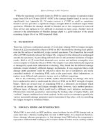
49 Analysing the infinite plate under uniform tension with a circular hole of diameter a, and subjected
to a uniform stress σ
0
, Fig. 9.4.
50 The peculiarity of this problem is that the far-field boundary conditions are better expressed in
cartesian coordinates, whereas the ones around the hole should be written in polar coordinate system.
51 We will solve this problem by replacing the plate with a thick tube subjected to two different set of
loads. The first one is a thick cylinder subjected to uniform radial pressure (solution of which is well

known from Strength of Materials), the second one is a thick cylinder subjected to both radial and shear
stresses which must be compatible with the traction applied on the rectangular plate.
52 First we select a stress function which satisfies the biharmonic Equation (Eq. ??), and the far-field
boundary conditions. From St Venant principle, away from the hole, the boundary conditions are given
by:
σ
xx
= σ
0
; σ
yy
= τ
xy
= 0 (9.65)
53 Recalling (Eq. 9.19) that σ
xx
=
∂
2
Φ
∂y
2
, this would would suggest a stress function Φ of the form
Φ=σ
0
y
2
. Alternatively, the presence of the circular hole would suggest a polar representation of Φ.
Thus, substituting y = r sin θ would result in Φ = σ
0

r
2
sin
2
θ.
54 Since sin
2
θ =
1
2
(1 − cos 2θ), we could simplify the stress function into
Φ=f(r)cos2θ (9.66)
55 Substituting this function into the biharmonic equation (Eq. ??) yields

∂
2
∂r
2
+
1
r
∂
∂r
+
1
r
2
∂
2
∂θ

2

∂
2
Φ
∂r
2
+
1
r
∂Φ
∂r
+
1
r
2
∂
2
Φ
∂θ
2

= 0 (9.67-a)

d
2
dr
2
+
1

r
d
dr
−
4
r
2

d
2
f
dr
2
+
1
r
df
dr
−
4f
r
2

= 0 (9.67-b)
(note that the cos 2θ term is dropped)
56 The general solution of this ordinary linear fourth order differential equation is
f(r)=Ar
2
+ Br
4

+ C
1
r
2
+ D (9.68)
Victor Saouma Mechanics of Materials II
Draft
9.3 Circular Hole, (Kirsch, 1898) 11
thus the stress function becomes
Φ=

Ar
2
+ Br
4
+ C
1
r
2
+ D

cos 2θ (9.69)
57 Next, we must determine the constants A, B, C,andD. Using Eq. ??, the stresses are given by
σ
rr
=
1
r
∂Φ
∂r

+
1
r
2
∂
2
Φ
∂θ
2
= −

2A +
6C
r
4
+
4D
r
2

cos 2θ
σ
θθ
=
∂
2
Φ
∂r
2
=


2A +12Br
2
+
6C
r
4

cos 2θ
τ
rθ
= −
∂
∂r

1
r
∂Φ
∂θ

=

2A +6Br
2
−
6C
r
4
−
2D

r
2

sin 2θ
(9.70)
58 Next we seek to solve for the four constants of integration by applying the boundary conditions. We
will identify two sets of boundary conditions:
1. Outer boundaries: around an infinitely large circle of radius b inside a plate subjected to uniform
stress σ
0
, the stresses in polar coordinates are obtained from Strength of Materials

σ
rr
σ
rθ
σ
rθ
σ
θθ

=

cos θ −sin θ
sin θ cos θ

σ
0
0
00


cos θ −sin θ
sin θ cos θ

T
(9.71)
yielding (recalling that sin
2
θ =1/2sin2θ, and cos
2
θ =1/2(1 + cos 2θ)).
(σ
rr
)
r=b
= σ
0
cos
2
θ =
1
2
σ
0
(1 + cos 2θ) (9.72-a)
(σ
rθ
)
r=b
=

1
2
σ
0
sin 2θ (9.72-b)
(σ
θθ
)
r=b
=
σ
0
2
(1 − cos 2θ) (9.72-c)
For reasons which will become apparent later, it is more convenient to decompose the state of
stress given by Eq. 9.72-a and 9.72-b, into state I and II:
(σ
rr
)
I
r=b
=
1
2
σ
0
(9.73-a)
(σ
rθ
)

I
r=b
= 0 (9.73-b)
(σ
rr
)
II
r=b
=
1
2
σ
0
cos 2θ
✛
(9.73-c)
(σ
rθ
)
II
r=b
=
1
2
σ
0
sin 2θ
✛
(9.73-d)
Where state I corresponds to a thick cylinder with external pressure applied on r = b and of

magnitude σ
0
/2. Hence, only the last two equations will provide us with boundary conditions.
2. Around the hole: the stresses should be equal to zero:
(σ
rr
)
r=a
=0
✛
(9.74-a)
(σ
rθ
)
r=a
=0
✛
(9.74-b)
59 Upon substitution in Eq. 9.70 the four boundary conditions (Eq. 9.73-c, 9.73-d, 9.74-a, and 9.74-b)
become
−

2A +
6C
b
4
+
4D
b
2


=
1
2
σ
0
(9.75-a)

2A +6Bb
2
−
6C
b
4
−
2D
b
2

=
1
2
σ
0
(9.75-b)
−

2A +
6C
a

4
+
4D
a
2

= 0 (9.75-c)

2A +6Ba
2
−
6C
a
4
−
2D
a
2

= 0 (9.75-d)
Victor Saouma Mechanics of Materials II
Draft
12 SOME ELASTICITY PROBLEMS
60 Solving for the four unknowns, and taking
a
b
= 0 (i.e. an infinite plate), we obtain:
A = −
σ
0

4
; B =0; C = −
a
4
4
σ
0
; D =
a
2
2
σ
0
(9.76)
61 To this solution, we must superimpose the one of a thick cylinder subjected to a uniform radial traction
σ
0
/2 on the outer surface, and with b much greater than a (Eq. 9.73-a and 9.73-b. These stresses are
obtained from Strength of Materials yielding for this problem (carefull about the sign)
σ
rr
=
σ
0
2

1 −
a
2
r

2

(9.77-a)
σ
θθ
=
σ
0
2

1+
a
2
r
2

(9.77-b)
62 Thus, substituting Eq. 9.75-a- into Eq. 9.70, we obtain
σ
rr
=
σ
0
2

1 −
a
2
r
2


+

1+3
a
4
r
4
−
4a
2
r
2

1
2
σ
0
cos 2θ (9.78-a)
σ
θθ
=
σ
0
2

1+
a
2
r

2

−

1+
3a
4
r
4

1
2
σ
0
cos 2θ (9.78-b)
σ
rθ
= −

1 −
3a
4
r
4
+
2a
2
r
2


1
2
σ
0
sin 2θ (9.78-c)
63 We observe that as r →∞, both σ
rr
and σ
rθ
are equal to the values given in Eq. 9.72-a and 9.72-b
respectively.
64 Alternatively, at the edge of the hole when r = a we obtain
σ
rr
= 0 (9.79)
σ
rθ
= 0 (9.80)
σ
θθ
|
r=a
= σ
0
(1 − 2cos2θ) (9.81)
which for θ =
π
2
and
3π

2
gives a stress concentration factor (SCF) of 3. For θ =0andθ = π, σ
θθ
= −σ
0
.
Victor Saouma Mechanics of Materials II
Draft
Part III
FRACTURE MECHANICS
Draft
Draft
Chapter 10
ELASTICITY BASED SOLUTIONS
FOR CRACK PROBLEMS
1 Following the solution for the stress concentration around a circular hole, and as a transition from
elasticity to fracture mechanics, we now examine the stress field around a sharp crack. This problem,
first addressed by Westergaard, is only one in a long series of similar ones, Table 10.1.
Problem Coordinate System Real/Complex Solution Date
Circular Hole Polar Real Kirsh 1898
Elliptical Hole Curvilinear Complex Inglis 1913
Crack Cartesian Complex Westergaard 1939
V Notch Polar Complex Willimas 1952
Dissimilar Materials Polar Complex Williams 1959
Anisotropic Materials Cartesian Complex Sih 1965
Table 10.1: Summary of Elasticity Based Problems Analysed
2 But first, we need to briefly review complex variables, and the formulation of the Airy stress functions
in the complex space.
10.1 †Complex Variables
3 In the preceding chapter, we have used the Airy stress function with real variables to determine the

stress field around a circular hole, however we need to extend Airy stress functions to complex variables
in order to analyze stresses at the tip of a crack.
4 First we define the complex number z as:
z = x
1
+ ix
2
= re
iθ
(10.1)
where i =
√
−1, x
1
and x
2
are the cartesian coordinates, and r and θ are the polar coordinates.
5 We further define an analytic function, f (z) one which derivatives depend only on z. Applying the
chain rule
∂
∂x
1
f(z)=
∂
∂z
f(z)
∂z
∂x
1
= f


(z)
∂z
∂x
1
= f

(z) (10.2-a)
Draft
2 ELASTICITY BASED SOLUTIONS FOR CRACK PROBLEMS
∂
∂x
2
f(z)=
∂
∂z
f(z)
∂z
∂x
2
= f

(z)
∂z
∂x
2
= if

(z) (10.2-b)
6 If f(z)=α + iβ where α and β are real functions of x

1
and x
2
,andf(z) is analytic, then from Eq.
10.2-a and 10.2-b we have:
∂f(z)
∂x
1
=
∂α
∂x
1
+ i
∂β
∂x
1
= f

(z)
∂f(z)
∂x
2
=
∂α
∂x
2
+ i
∂β
∂x
2

= if

(z)

i

∂α
∂x
1
+ i
∂β
∂x
1

=
∂α
∂x
2
+ i
∂β
∂x
2
(10.3)
7 Equating the real and imaginary parts yields the Cauchy-Riemann equations:
∂α
∂x
1
=
∂β
∂x

2
;
∂α
∂x
2
= −
∂β
∂x
1
(10.4)
8 If we differentiate those two equation, first with respect to x
1
, then with respect to x
2
, and then add
them up we obtain
∂
2
α
∂x
2
1
+
∂
2
α
∂x
2
2
=0 or ∇

2
(α)=0
(10.5)
which is Laplace’s equation.
9 Similarly we can have:
∇
2
(β) = 0 (10.6)
Hence both the real (α) and the immaginary part (β) of an analytic function will separately provide
solution to Laplace’s equation, and α and β are conjugate harmonic functions.
10.2 †Complex Airy Stress Functions
10 It can be shown that any stress function can be expressed as
Φ=Re[(x
1
− ix
2
)ψ(z)+χ(z)] (10.7)
provided that both ψ(z) (psi) and χ(z) (chi) are harmonic (i.e ∇
2
(ψ)=∇
2
(χ) = 0) analytic functions
of x
1
and x
2
. ψ and χ are often refered to as the Kolonov-Muskhelishvili complex potentials.
11 If f(z)=α + iβ and both α and β are real, then its conjugate function is defined as:
¯
f(¯z)=α −iβ

(10.8)
12 Note that conjugate functions should not be confused with the conjugate harmonic functions. Hence
we can rewrite Eq. 10.7 as:
Φ=Re[¯zψ(z)+χ(z)]
(10.9)
13 Substituting Eq. 10.9 into Eq. 9.19, we can determine the stresses
σ
11
+ σ
22
=4Reψ

(z) (10.10)
σ
22
− σ
11
+2iσ
12
=2[¯zψ

(z)+χ

(z)] (10.11)
and by separation of real and imaginary parts we can then solve for σ
22
− σ
11
& σ
12

.
14 Displacements can be similarly obtained.
Victor Saouma Mechanics of Materials II
Draft
10.3 Crack in an Infinite Plate, (Westergaard, 1939) 3
σ
σ
σ
σ
x
x
0
0
0
0
1
2
2a
Figure 10.1: Crack in an Infinite Plate
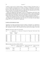
10.3 Crack in an Infinite Plate, (Westergaard, 1939)
15 Just as both Kolosoff (1910) and Inglis (1913) independently solved the problem of an elliptical hole,
there are two classical solutions for the crack problem. The first one was proposed by Westergaard, and
the later by Williams. Whereas the first one is simpler to follow, the second has the advantage of being
extended to cracks at the interface of two different homogeneous isotropic materials and be applicable
for V notches.
16 Let us consider an infinite plate subjected to uniform biaxial stress σ
0
with a central crack of length
2a, Fig. 10.1. From Inglis solution, we know that there would be a theoretically infinite stress at the tip
of the crack, however neither the nature of the singularity nor the stress field can be derived from it.

17 Westergaard’s solution, (Westergaard 1939) starts by assuming Φ(z) as a harmonic function (thus
satisfying Laplace’s equation ∇
2
(Φ) = 0). Denoting by φ

(z)andφ

(z) the first and second derivatives
respectively, and
¯
φ(z)and
¯
¯
φ(z) its first and second integrals respectively of the function φ(z).
18 Westergaard has postulated that
Φ=Re
¯
¯
φ(z)+x
2
Im
¯
φ(z) (10.12)
is a solution to the crack problem
1
.
19 †Let us verify that Φ satisfies the biharmonic equation. Taking the first derivatives, and recalling
from from Eq. 10.2-a that
∂
∂x

1
f(z)=f

(z), we have
∂Φ
∂x
1
=
∂
∂x
1

Re
¯
¯
φ

+




x
2
∂
∂x
1
Im
¯
φ(z)+Im

¯
φ(z)
∂x
2
∂x
1

0




(10.13-a)
=Re
¯
φ(z)+x
2
Imφ(z) (10.13-b)
σ
22
=
∂
2
Φ
∂x
2
1
=
∂
∂x

1

Re
¯
φ(z)

+

x
2
∂
∂x
1
Imφ(z)+Imφ(z)
∂x
2
∂x
1

(10.13-c)
=Reφ(z)+x
2
Imφ

(z) (10.13-d)
1
Note that we should not confuse the Airy stress function Φ with the complex function φ(z).
Victor Saouma Mechanics of Materials II
Draft
4 ELASTICITY BASED SOLUTIONS FOR CRACK PROBLEMS

20 †Similarly, differentiating with respect to x
2
, and recalling from Eq. 10.2-b that
∂
∂x
2
f(z)=if

(z), we
obtain
∂Φ
∂x
2
=
∂
∂x
2
(Re
¯
¯
φ(z)+[x
2
∂
∂x
2

Im
¯
φ(z)


+
∂x
2
∂x
2
Im
¯
φ(z)] (10.14-a)
= −Im
¯
φ(z)+x
2
Reφ(z)+Im
¯
φ(z) (10.14-b)
σ
11
=
∂
2
Φ
∂x
2
2
= x
2
∂
∂x
2
Reφ(z)+Reφ(z)

∂x
2
∂x
2
(10.14-c)
= −x
2
Imφ

(z)+Reφ(z) (10.14-d)
21 †Similarly, it can be shown that
σ
12
= −
∂
2
Φ
∂x
1
∂x
2
= −x
2
Reφ

(z) (10.15)
22 †Having derived expressions for the stresses and the second partial derivatives of Φ, substituting into
Eq. ??, it can be shown that the biharmonic equation is satisfied, thus Φ is a valid solution.
23 †If we want to convince ourselves that the stresses indeed satisfy both the equilibrium and compati-
bility equations (which they do by virtue of Φ satisfiying the bi-harmonic equation), we have from Eq.

6.18 in 2D:
1. Equilibrium:
∂σ
11
∂x
1
+
∂σ
12
∂x
2
= 0 (10.16-a)
∂σ
22
∂x
2
+
∂σ
12
∂x
1
= 0 (10.16-b)
Let us consider the first equation
∂σ
11
∂x
1
=
∂
∂x

1

∂
2
Φ
∂x
2
2

=
∂
∂x
1
[Reφ(z) −x
2
Imφ

(z)] (10.17-a)
=Reφ

(z) −x
2
Imφ

(z) (10.17-b)
∂σ
12
∂x
2
=

∂
∂x
2

∂
2
Φ
∂x
1
∂x
2

=
∂
∂x
2
[−x
2
Reφ

(z)] (10.17-c)
= −Reφ

(z)+x
2
∂
∂x
1
Imφ


(z) (10.17-d)
= −Reφ

(z)+x
2
Imφ

(z) (10.17-e)
If we substitute those two equations into Eq. 10.16-a then we do obtain zero. Similarly, it can
be shown that Eq. 10.16-b is satisfied.
2. Compatibility: In plane strain, displacements are given by
2µu
1
=(1− 2ν)Re
¯
φ(z) −x
2
Imφ(z) (10.18-a)
2µu
2
= 2(1 − ν)Im
¯
φ(z) −x
2
Re φ(z) (10.18-b)
and are obtained by integration of the strains which were in turn obtained from the stresses. As
a check we compute
2µε
11
=

∂u
1
∂x
1
(10.19-a)
=(1− 2ν)Reφ(z) − x
2
Imφ

(z) (10.19-b)
=(1− ν)[Reφ(z) −x
2
Imφ

(z)]

 
σ
11
−ν [Reφ(z)+x
2
Imφ

(z)]

 
σ
22
(10.19-c)
=(1− ν)σ

11
− νσ
22
(10.19-d)
Victor Saouma Mechanics of Materials II
Draft
10.3 Crack in an Infinite Plate, (Westergaard, 1939) 5
Recalling that
µ =
E
2(1 + ν)
(10.20)
then
Eε
11
=(1−ν
2
)σ
11
− ν(1 + ν)σ
22
(10.21)
this shows that Eε
11
= σ
11
−ν(σ
22
−σ
33

), and for plane strain, ε
33
=0⇒ σ
33
= ν(σ
11
+ σ
22
)and
Eε
11
=(1−ν
2
)σ
11
− ν(1 + ν)σ
22
24 So far Φ was defined independently of the problem, and we simply determined the stresses in terms
of it, and verified that the bi-harmonic equation was satisfied.
25 Next, we must determine φ such that the boundary conditions are satisfied. For reasons which will
become apparent later, we generalize our problem to one in which we have a biaxial state of stress applied
on the plate. Hence:
1. Along the crack: at x
2
=0and−a<x
1
<awe have σ
22
= 0 (traction free crack).
2. At infinity: at x

2
= ±∞, σ
22
= σ
0
We note from Eq. 10.13-d that at x
2
=0σ
22
reduces to
(σ
22
)
x
2
=0
=Reφ(z) (10.22)
26 Furthermore, we expect σ
22
→ σ
0
as x
1
→∞,andσ
22
to be greater than σ
0
when | x
1
− a |>(due

to anticipated singularity predicted by Inglis), thus a possible choice for σ
22
would be σ
22
=
σ
0
1−
a
x
1
,for
symmetry, this is extended to σ
22
=
σ
0

1−
a
2
x
2
1

. However, we also need to have σ
22
= 0 when x
2
=0and

−a<x
1
<a, thus the function φ(z) should become imaginary along the crack, and
σ
22
=Re


σ
0

1 −
a
2
x
2
1


(10.23)
27 Thus from Eq. 10.22 we have (note the transition from x
1
to z).
φ(z)=
σ
0

1 −
a
2

z
2
(10.24)
28 If we perform a change of variable and define η = z − a = re
iθ
and assuming
η
a
 1, and recalling
that e
iθ
=cosθ + i sin θ, then the first term of Eq. 10.13-d can be rewritten as
Reφ(z)=Re
σ
0

η
2
+2aη
η
2
+a
2
+2aη
≈ Re
σ
0

2aη
a

2
≈ Reσ
0

a
2η
≈ Reσ
0

a
2re
iθ
≈ σ
0

a
2r
e
−i
θ
2
≈ σ
0

a
2r
cos
θ
2
(10.25-a)

29 Recalling that sin 2θ =2sinθ cos θ and that e
−iθ
=cosθ −i sin θ, we substituting x
2
= r sin θ into the
second term
x
2
Imφ

= r sin θIm
σ
0
2

a
2(re
iθ
)
3
= σ
0

a
2r
sin
θ
2
cos
θ

2
sin
3θ
2
(10.26)
30 Combining the above equations, with Eq. 10.13-d, 10.14-d, and 10.15 we obtain
Victor Saouma Mechanics of Materials II
Draft
6 ELASTICITY BASED SOLUTIONS FOR CRACK PROBLEMS
σ
22
= σ
0

a
2r
cos
θ
2

1+sin
θ
2
sin
3θ
2

+ ··· (10.27)
σ
11

= σ
0

a
2r
cos
θ
2

1 − sin
θ
2
sin
3θ
2

+ ··· (10.28)
σ
12
= σ
0

a
2r
sin
θ
2
cos
θ
2

cos
3θ
2
+ ··· (10.29)
31 Recall that this was the biaxial case, the uniaxial case may be reproduced by superimposing a pressure
in the x
1
direction equal to −σ
0
, however this should not affect the stress field close to the crack tip.
32 Using a similar approach, we can derive expressions for the stress field around a crack tip in a plate
subjected to far field shear stresses (mode II as defined later) using the following expression of φ
Φ
II
(z)=−x
2
Re
¯
φ
II
(z) ⇒ φ
II
=
τ

1 −
a
2
z
2

(10.30)
and for the same crack but subjected to antiplane shear stresses (mode III)
Φ

III
(z)=
σ
13

1 −
a
2
z
2
(10.31)
10.4 Stress Intensity Factors (Irwin)
33 Irwin
2
(Irwin 1957) introduced the concept of stress intensity factor defined as:



K
I
K
II
K
III




= lim
r→0,θ=0
√
2πr



σ
22
σ
12
σ
23



(10.32)
where σ
ij
are the near crack tip stresses, and K
i
are associated with three independent kinematic
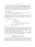
movements of the upper and lower crack surfaces with respect to each other, as shown in Fig. 10.2:
• Opening Mode, I: The two crack surfaces are pulled apart in the y direction, but the deformations
are symmetric about the x − z and x − y planes.
• Shearing Mode, II: The two crack surfaces slide over each other in the x-direction, but the defor-
mations are symmetric about the x − y plane and skew symmetric about the x − z plane.
• Tearing Mode, III: The crack surfaces slide over each other in the z-direction, but the deformations
are skew symmetric about the x − y and x − z planes.

34 From Eq. 10.27, 10.28 and 10.29 with θ =0,wehave
K
I
=
√
2πrσ
22
=
√
2πrσ
0

a
2r
= σ
0
√
πa (10.33-a)
where r is the length of a small vector extending directly forward from the crack tip.
2
Irwin was asked by the Office of Naval Research (ONR) to investigate the Liberty ships failure during World War II,
just as thirty years earlier Inglis was investigating the failure of British ships.
Victor Saouma Mechanics of Materials II
Draft
10.5 Near Crack Tip Stresses and Displacements in Isotropic Cracked Solids 7
Figure 10.2: Independent Modes of Crack Displacements
35 Thus stresses and displacements can all be rewritten in terms of the SIF




σ
22
σ
12
σ
23



=
1
√
2πr


f
I
11
(θ) f
II
11
(θ) f
III
11
(θ)
f
I
22
(θ) f
II

22
(θ) f
III
22
(θ)
f
I
12
(θ) f
II
12
(θ) f
III
12
(θ)





K
I
K
II
K
III



(10.34-a)

i.e.
σ
12
=
K
II
√
2πr
sin
θ
2
cos
θ
2
cos
3θ
2

 
f
II
22
(10.35)
1. Since higher order terms in r were neglected, previous equations are exact in the limit as r → 0
2. Distribution of elastic stress field at tip can be described by K
I
,K
II
and K
III

. Note that this
polar distribution is identical for all cases. As we shall see later, for anisotropic cases, the spatial
distribution is a function of elastic constants.
3. SIF are additives, i.e.
4. The SIF is the measure of the strength of the singularity (analogous to SCF)
5. K = f(g)σ
√
πa where f(g) is a parameter
3
that depends on the specimen, crack geometry, and
loading.
6. Tada “Stress Analysis of Cracks”, (Tada, Paris and Irwin 1973); and Cartwright & Rooke, “Com-
pendium of Stress Intensity Factors” (Rooke and Cartwright 1976).
7. One of the underlying principles of FM is that unstable fracture occurs when the SIF reaches
a critical value K
Ic
. K
Ic
or fracture toughness represents the inherent ability of a material to
withstand a given stress field intensity at the tip of a crack and to resist progressive tensile crack
extensions.
10.5 Near Crack Tip Stresses and Displacements in Isotropic
Cracked Solids
36 Using Irwin’s concept of the stress intensity factors, which characterize the strength of the singularity
at a crack tip, the near crack tip (r  a) stresses and displacements are always expressed as:
3
Note that in certain literature, (specially the one of Lehigh University), instead of K = f(g)σ
√
πa, k = f (g)σ
√

a is
used.
Victor Saouma Mechanics of Materials II
Draft
8 ELASTICITY BASED SOLUTIONS FOR CRACK PROBLEMS
Pure mode I loading:
σ
xx
=
K
I
(2πr)
1
2
cos
θ
2

1 − sin
θ
2
sin
3θ
2

(10.36-a)
σ
yy
=
K

I
(2πr)
1
2
cos
θ
2

1+sin
θ
2
sin
3θ
2

(10.36-b)
τ
xy
=
K
I
(2πr)
1
2
sin
θ
2
cos
θ
2

cos
3θ
2
(10.36-c)
σ
zz
= ν(σ
x
+ σ
y
)τ
xz
= τ
yz
= 0 (10.36-d)
u =
K
I
2µ

r
2π

1
2
cos
θ
2

κ − 1+2sin

2
θ
2

(10.36-e)
v =
K
I
2µ

r
2π

1
2
sin
θ
2

κ +1− 2cos
2
θ
2

(10.36-f)
w = 0 (10.36-g)
Pure mode II loading:
σ
xx
= −

K
II
(2πr)
1
2
sin
θ
2

2 + cos
θ
2
cos
3θ
2

(10.37-a)
σ
yy
=
K
II
(2πr)
1
2
sin
θ
2
cos
θ

2
cos
3θ
2
(10.37-b)
τ
xy
=
K
II
(2πr)
1
2
cos
θ
2

1 − sin
θ
2
sin
3θ
2

(10.37-c)
σ
zz
= ν(σ
x
+ σ

y
) (10.37-d)
τ
xz
= τ
yz
= 0 (10.37-e)
u =
K
II
2µ

r
2π

1
2
sin
θ
2

κ +1+2cos
2
θ
2

(10.37-f)
v = −
K
II

2µ

r
2π

1
2
cos
θ
2

κ − 1 − 2sin
2
θ
2

(10.37-g)
w = 0 (10.37-h)
Pure mode III loading:
τ
xz
= −
K
III
(2πr)
1
2
sin
θ
2

(10.38-a)
τ
yz
=
K
III
(2πr)
1
2
cos
θ
2
(10.38-b)
σ
xx
= σ
y
= σ
z
= τ
xy
= 0 (10.38-c)
w =
K
III
µ

2r
π


1
2
sin
θ
2
(10.38-d)
u = v = 0 (10.38-e)
where κ =3−4ν for plane strain, and κ =
3−ν
1+ν
for plane stress.
37 Using Eq. ??, ??,and?? we can write the stresses in polar coordinates
Victor Saouma Mechanics of Materials II