Information Theory, Inference, and Learning Algorithms phần 8 docx
Bạn đang xem bản rút gọn của tài liệu. Xem và tải ngay bản đầy đủ của tài liệu tại đây (1.7 MB, 64 trang )
Copyright Cambridge University Press 2003. On-screen viewing permitted. Printing not permitted. />You can buy this book for 30 pounds or $50. See for links.
34
Independent Component Analysis and
Latent Variable Modelling
34.1 Latent variable models
Many statistical models are generative models (that is, models that specify
a full probability density over all variables in the situation) that make use of
latent variables to describe a probability distribution over observables.
Examples of latent variable models include Chapter 22’s mixture models,
which model the observables as coming from a superposed mixture of simple
probability distributions (the latent variables are the unknown class labels
of the examples); hidden Markov models (Rabiner and Juang, 1986; Durbin
et al., 1998); and factor analysis.
The decoding problem for error-correcting codes can also be viewed in
terms of a latent variable model – figure 34.1. In that case, the encoding
matrix G is normally known in advance. In latent variable modelling, the
parameters equivalent to G are usually not known, and must be inferred from
the data along with the latent variables s.
y
N
y
1
G
s
K
s
1
Figure 34.1. Error-correcting
codes as latent variable models.
The K latent variables are the
independent source bits
s
1
, . . . , s
K
; these give rise to the
observables via the generator
matrix G.
Usually, the latent variables have a simple distribution, often a separable
distribution. Thus when we fit a latent variable model, we are finding a de-
scription of the data in terms of ‘independent components’. The ‘independent
component analysis’ algorithm corresponds to perhaps the simplest possible
latent variable model with continuous latent variables.
34.2 The generative model for independent component analysis
A set of N observations D = {x
(n)
}
N
n=1
are assumed to be generated as follows.
Each J-dimensional vector x is a linear mixture of I underlying source signals,
s:
x = Gs, (34.1)
where the matrix of mixing coefficients G is not known.
The simplest algorithm results if we assume that the number of sources
is equal to the number of observations, i.e., I = J. Our aim is to recover
the source variables s (within some multiplicative factors, and possibly per-
muted). To put it another way, we aim to create the inverse of G (within a
post-multiplicative factor) given only a set of examples {x}. We assume that
the latent variables are independently distributed, with marginal distributions
P (s
i
|H) ≡ p
i
(s
i
). Here H denotes the assumed form of this model and the
assumed probability distributions p
i
of the latent variables.
The probability of the observables and the hidden variables, given G and
437
Copyright Cambridge University Press 2003. On-screen viewing permitted. Printing not permitted. />You can buy this book for 30 pounds or $50. See for links.
438 34 — Independent Component Analysis and Latent Variable Modelling
H, is:
P ({x
(n)
, s
(n)
}
N
n=1
|G, H) =
N
n=1
P (x
(n)
|s
(n)
, G, H)P(s
(n)
|H)
(34.2)
=
N
n=1
j
δ
x
(n)
j
−
i
G
ji
s
(n)
i
i
p
i
(s
(n)
i
)
. (34.3)
We assume that the vector x is generated without noise. This assumption is
not usually made in latent variable modelling, since noise-free data are rare;
but it makes the inference problem far simpler to solve.
The likelihood function
For learning about G from the data D, the relevant quantity is the likelihood
function
P (D |G, H) =
n
P (x
(n)
|G, H) (34.4)
which is a product of factors each of which is obtained by marginalizing over
the latent variables. When we marginalize over delta functions, remember
that
ds δ(x − vs)f(s) =
1
v
f(x/v). We adopt summation convention at this
point, such that, for example, G
ji
s
(n)
i
≡
i
G
ji
s
(n)
i
. A single factor in the
likelihood is given by
P (x
(n)
|G, H) =
d
I
s
(n)
P (x
(n)
|s
(n)
, G, H)P(s
(n)
|H) (34.5)
=
d
I
s
(n)
j
δ
x
(n)
j
− G
ji
s
(n)
i
i
p
i
(s
(n)
i
) (34.6)
=
1
|det G|
i
p
i
(G
−1
ij
x
j
) (34.7)
⇒ ln P(x
(n)
|G, H) = −ln |det G| +
i
ln p
i
(G
−1
ij
x
j
). (34.8)
To obtain a maximum likelihood algorithm we find the gradient of the log
likelihood. If we introduce W ≡ G
−1
, the log likelihood contributed by a
single example may be written:
ln P (x
(n)
|G, H) = ln |det W|+
i
ln p
i
(W
ij
x
j
). (34.9)
We’ll assume from now on that det W is positive, so that we can omit the
absolute value sign. We will need the following identities:
∂
∂G
ji
ln det G = G
−1
ij
= W
ij
(34.10)
∂
∂G
ji
G
−1
lm
= −G
−1
lj
G
−1
im
= −W
lj
W
im
(34.11)
∂
∂W
ij
f = −G
jm
∂
∂G
lm
f
G
li
. (34.12)
Let us define a
i
≡ W
ij
x
j
,
φ
i
(a
i
) ≡ d ln p
i
(a
i
)/da
i
, (34.13)
Copyright Cambridge University Press 2003. On-screen viewing permitted. Printing not permitted. />You can buy this book for 30 pounds or $50. See for links.
34.2: The generative model for independent component analysis 439
Repeat for each datapoint x:
1. Put x through a linear mapping:
a = Wx.
2. Put a through a nonlinear map:
z
i
= φ
i
(a
i
),
where a popular choice for φ is φ = −tanh(a
i
).
3. Adjust the weights in accordance with
∆W ∝ [W
T
]
−1
+ zx
T
.
Algorithm 34.2. Independent
component analysis – online
steepest ascents version.
See also algorithm 34.4, which is
to be preferred.
and z
i
= φ
i
(a
i
), which indicates in which direction a
i
needs to change to make
the probability of the data greater. We may then obtain the gradient with
respect to G
ji
using equations (34.10) and (34.11):
∂
∂G
ji
ln P (x
(n)
|G, H) = −W
ij
− a
i
z
i
W
i
j
. (34.14)
Or alternatively, the derivative with respect to W
ij
:
∂
∂W
ij
ln P (x
(n)
|G, H) = G
ji
+ x
j
z
i
. (34.15)
If we choose to change W so as to ascend this gradient, we obtain the learning
rule
∆W ∝ [W
T
]
−1
+ zx
T
. (34.16)
The algorithm so far is summarized in algorithm 34.2.
Choices of φ
The choice of the function φ defines the assumed prior distribution of the
latent variable s.
Let’s first consider the linear choice φ
i
(a
i
) = −κa
i
, which implicitly (via
equation 34.13) assumes a Gaussian distribution on the latent variables. The
Gaussian distribution on the latent variables is invariant under rotation of the
latent variables, so there can be no evidence favouring any particular alignment
of the latent variable space. The linear algorithm is thus uninteresting in that
it will never recover the matrix G or the original sources. Our only hope is
thus that the sources are non-Gaussian. Thankfully, most real sources have
non-Gaussian distributions; often they have heavier tails than Gaussians.
We thus move on to the popular tanh nonlinearity. If
φ
i
(a
i
) = −tanh(a
i
) (34.17)
then implicitly we are assuming
p
i
(s
i
) ∝ 1/ cosh(s
i
) ∝
1
e
s
i
+ e
−s
i
. (34.18)
This is a heavier-tailed distribution for the latent variables than the Gaussian
distribution.
Copyright Cambridge University Press 2003. On-screen viewing permitted. Printing not permitted. />You can buy this book for 30 pounds or $50. See for links.
440 34 — Independent Component Analysis and Latent Variable Modelling
(a)
x20
4
2
0
-2
-4
x1
0
42
0-2
-4
(b)
x20
4
2
0
-2
-4
x1
0
42
0-2
-4
(c)
x20
8
6
4
2
0
-2
-4
-6
-8
x1
0
8642
0-2-4-6
-8
(d)
x1
0 3020100-10-20-30
x2 0
30
20
10
0
-10
-20
-30
Figure 34.3. Illustration of the
generative models implicit in the
learning algorithm.
(a) Distributions over two
observables generated by 1/ cosh
distributions on the latent
variables, for G =
3/4 1/2
1/2 1
(compact distribution) and
G =
2 −1
−1 3/2
(broader
distribution). (b) Contours of the
generative distributions when the
latent variables have Cauchy
distributions. The learning
algorithm fits this amoeboid
object to the empirical data in
such a way as to maximize the
likelihood. The contour plot in
(b) does not adequately represent
this heavy-tailed distribution.
(c) Part of the tails of the Cauchy
distribution, giving the contours
0.01 . . . 0.1 times the density at
the origin. (d) Some data from
one of the generative distributions
illustrated in (b) and (c). Can you
tell which? 200 samples were
created, of which 196 fell in the
plotted region.
We could also use a tanh nonlinearity with gain β, that is, φ
i
(a
i
) =
−tanh(βa
i
), whose implicit probabilistic model is p
i
(s
i
) ∝ 1/[cosh(βs
i
)]
1/β
. In
the limit of large β, the nonlinearity becomes a step function and the probabil-
ity distribution p
i
(s
i
) becomes a biexponential distribution, p
i
(s
i
) ∝ exp(−|s|).
In the limit β → 0, p
i
(s
i
) approaches a Gaussian with mean zero and variance
1/β. Heavier-tailed distributions than these may also be used. The Student
and Cauchy distributions spring to mind.
Example distributions
Figures 34.3(a–c) illustrate typical distributions generated by the independent
components model when the components have 1/ cosh and Cauchy distribu-
tions. Figure 34.3d shows some samples from the Cauchy model. The Cauchy
distribution, being the more heavy-tailed, gives the clearest picture of how the
predictive distribution depends on the assumed generative parameters G.
34.3 A covariant, simpler, and faster learning algorithm
We have thus derived a learning algorithm that performs steepest descents
on the likelihood function. The algorithm does not work very quickly, even
on toy data; the algorithm is ill-conditioned and illustrates nicely the general
advice that, while finding the gradient of an objective function is a splendid
idea, ascending the gradient directly may not be. The fact that the algorithm is
ill-conditioned can be seen in the fact that it involves a matrix inverse, which
can be arbitrarily large or even undefined.
Covariant optimization in general
The principle of covariance says that a consistent algorithm should give the
same results independent of the units in which quantities are measured (Knuth,
Copyright Cambridge University Press 2003. On-screen viewing permitted. Printing not permitted. />You can buy this book for 30 pounds or $50. See for links.
34.3: A covariant, simpler, and faster learning algorithm 441
1968). A prime example of a non-covariant algorithm is the popular steepest
descents rule. A dimensionless objective function L(w) is defined, its deriva-
tive with respect to some parameters w is computed, and then w is changed
by the rule
∆w
i
= η
∂L
∂w
i
. (34.19)
This popular equation is dimensionally inconsistent: the left-hand side of this
equation has dimensions of [w
i
] and the right-hand side has dimensions 1/[w
i
].
The behaviour of the learning algorithm (34.19) is not covariant with respect
to linear rescaling of the vector w. Dimensional inconsistency is not the end of
the world, as the success of numerous gradient descent algorithms has demon-
strated, and indeed if η decreases with n (during on-line learning) as 1/n then
the Munro–Robbins theorem (Bishop, 1992, p. 41) shows that the parameters
will asymptotically converge to the maximum likelihood parameters. But the
non-covariant algorithm may take a very large number of iterations to achieve
this convergence; indeed many former users of steepest descents algorithms
prefer to use algorithms such as conjugate gradients that adaptively figure
out the curvature of the objective function. The defense of equation (34.19)
that points out η could be a dimensional constant is untenable if not all the
parameters w
i
have the same dimensions.
The algorithm would be covariant if it had the form
∆w
i
= η
i
M
ii
∂L
∂w
i
, (34.20)
where M is a positive-definite matrix whose i, i
element has dimensions [w
i
w
i
].
From where can we obtain such a matrix? Two sources of such matrices are
metrics and curvatures.
Metrics and curvatures
If there is a natural metric that defines distances in our parameter space w,
then a matrix M can be obtained from the metric. There is often a natural
choice. In the special case where there is a known quadratic metric defining
the length of a vector w, then the matrix can be obtained from the quadratic
form. For example if the length is w
2
then the natural matrix is M = I, and
steepest descents is appropriate.
Another way of finding a metric is to look at the curvature of the objective
function, defining A ≡ −∇∇L (where ∇ ≡ ∂/∂w). Then the matrix M =
A
−1
will give a covariant algorithm; what is more, this algorithm is the Newton
algorithm, so we recognize that it will alleviate one of the principal difficulties
with steepest descents, namely its slow convergence to a minimum when the
objective function is at all ill-conditioned. The Newton algorithm converges
to the minimum in a single step if L is quadratic.
In some problems it may be that the curvature A consists of both data-
dependent terms and data-independent terms; in this case, one might choose
to define the metric using the data-independent terms only (Gull, 1989). The
resulting algorithm will still be covariant but it will not implement an exact
Newton step. Obviously there are many covariant algorithms; there is no
unique choice. But covariant algorithms are a small subset of the set of all
algorithms!
Copyright Cambridge University Press 2003. On-screen viewing permitted. Printing not permitted. />You can buy this book for 30 pounds or $50. See for links.
442 34 — Independent Component Analysis and Latent Variable Modelling
Back to independent component analysis
For the present maximum likelihood problem we have evaluated the gradient
with respect to G and the gradient with respect to W = G
−1
. Steepest
ascents in W is not covariant. Let us construct an alternative, covariant
algorithm with the help of the curvature of the log likelihood. Taking the
second derivative of the log likelihood with respect to W we obtain two terms,
the first of which is data-independent:
∂G
ji
∂W
kl
= −G
jk
G
li
, (34.21)
and the second of which is data-dependent:
∂(z
i
x
j
)
∂W
kl
= x
j
x
l
δ
ik
z
i
, (no sum over i) (34.22)
where z
is the derivative of z. It is tempting to drop the data-dependent term
and define the matrix M by [M
−1
]
(ij)(kl)
= [G
jk
G
li
]. However, this matrix
is not positive definite (it has at least one non-positive eigenvalue), so it is
a poor approximation to the curvature of the log likelihood, which must be
positive definite in the neighbourhood of a maximum likelihood solution. We
must therefore consult the data-dependent term for inspiration. The aim is
to find a convenient approximation to the curvature and to obtain a covariant
algorithm, not necessarily to implement an exact Newton step. What is the
average value of x
j
x
l
δ
ik
z
i
? If the true value of G is G
∗
, then
x
j
x
l
δ
ik
z
i
=
G
∗
jm
s
m
s
n
G
∗
ln
δ
ik
z
i
. (34.23)
We now make several severe approximations: we replace G
∗
by the present
value of G, and replace the correlated average s
m
s
n
z
i
by s
m
s
n
z
i
≡
Σ
mn
D
i
. Here Σ is the variance–covariance matrix of the latent variables
(which is assumed to exist), and D
i
is the typical value of the curvature
d
2
ln p
i
(a)/da
2
. Given that the sources are assumed to be independent, Σ
and D are both diagonal matrices. These approximations motivate the ma-
trix M given by:
[M
−1
]
(ij)(kl)
= G
jm
Σ
mn
G
ln
δ
ik
D
i
, (34.24)
that is,
M
(ij)(kl)
= W
mj
Σ
−1
mn
W
nl
δ
ik
D
−1
i
. (34.25)
For simplicity, we further assume that the sources are similar to each other so
that Σ and D are both homogeneous, and that ΣD = 1. This will lead us to
an algorithm that is covariant with respect to linear rescaling of the data x,
but not with respect to linear rescaling of the latent variables. We thus use:
M
(ij)(kl)
= W
mj
W
ml
δ
ik
. (34.26)
Multiplying this matrix by the gradient in equation (34.15) we obtain the
following covariant learning algorithm:
∆W
ij
= η
W
ij
+ W
i
j
a
i
z
i
. (34.27)
Notice that this expression does not require any inversion of the matrix W.
The only additional computation once z has been computed is a single back-
ward pass through the weights to compute the quantity
x
j
= W
i
j
a
i
(34.28)
Copyright Cambridge University Press 2003. On-screen viewing permitted. Printing not permitted. />You can buy this book for 30 pounds or $50. See for links.
34.3: A covariant, simpler, and faster learning algorithm 443
Repeat for each datapoint x:
1. Put x through a linear mapping:
a = Wx.
2. Put a through a nonlinear map:
z
i
= φ
i
(a
i
),
where a popular choice for φ is φ = −tanh(a
i
).
3. Put a back through W:
x
= W
T
a.
4. Adjust the weights in accordance with
∆W ∝ W + zx
T
.
Algorithm 34.4. Independent
component analysis – covariant
version.
in terms of which the covariant algorithm reads:
∆W
ij
= η
W
ij
+ x
j
z
i
. (34.29)
The quantity
W
ij
+ x
j
z
i
on the right-hand side is sometimes called the
natural gradient. The covariant independent component analysis algorithm is
summarized in algorithm 34.4.
Further reading
ICA was originally derived using an information maximization approach (Bell
and Sejnowski, 1995). Another view of ICA, in terms of energy functions,
which motivates more general models, is given by Hinton et al. (2001). Another
generalization of ICA can be found in Pearlmutter and Parra (1996, 1997).
There is now an enormous literature on applications of ICA. A variational free
energy minimization approach to ICA-like models is given in (Miskin, 2001;
Miskin and MacKay, 2000; Miskin and MacKay, 2001). Further reading on
blind separation, including non-ICA algorithms, can be found in (Jutten and
Herault, 1991; Comon et al., 1991; Hendin et al., 1994; Amari et al., 1996;
Hojen-Sorensen et al., 2002).
Infinite models
While latent variable models with a finite number of latent variables are widely
used, it is often the case that our beliefs about the situation would be most
accurately captured by a very large number of latent variables.
Consider clustering, for example. If we attack speech recognition by mod-
elling words using a cluster model, how many clusters should we use? The
number of possible words is unbounded (section 18.2), so we would really like
to use a model in which it’s always possible for new clusters to arise.
Furthermore, if we do a careful job of modelling the cluster corresponding
to just one English word, we will probably find that the cluster for one word
should itself be modelled as composed of clusters – indeed, a hierarchy of
Copyright Cambridge University Press 2003. On-screen viewing permitted. Printing not permitted. />You can buy this book for 30 pounds or $50. See for links.
444 34 — Independent Component Analysis and Latent Variable Modelling
clusters within clusters. The first levels of the hierarchy would divide male
speakers from female, and would separate speakers from different regions –
India, Britain, Europe, and so forth. Within each of those clusters would be
subclusters for the different accents within each region. The subclusters could
have subsubclusters right down to the level of villages, streets, or families.
Thus we would often like to have infinite numbers of clusters; in some
cases the clusters would have a hierarchical structure, and in other cases the
hierarchy would be flat. So, how should such infinite models be implemented
in finite computers? And how should we set up our Bayesian models so as to
avoid getting silly answers?
Infinite mixture models for categorical data are presented in Neal (1991),
along with a Monte Carlo method for simulating inferences and predictions.
Infinite Gaussian mixture models with a flat hierarchical structure are pre-
sented in Rasmussen (2000). Neal (2001) shows how to use Dirichlet diffusion
trees to define models of hierarchical clusters. Most of these ideas build on
the Dirichlet process (section 18.2). This remains an active research area
(Rasmussen and Ghahramani, 2002; Beal et al., 2002).
34.4 Exercises
Exercise 34.1.
[3 ]
Repeat the derivation of the algorithm, but assume a small
amount of noise in x: x = Gs + n; so the term δ
x
(n)
j
−
i
G
ji
s
(n)
i
in the joint probability (34.3) is replaced by a probability distribution
over x
(n)
j
with mean
i
G
ji
s
(n)
i
. Show that, if this noise distribution has
sufficiently small standard deviation, the identical algorithm results.
Exercise 34.2.
[3 ]
Implement the covariant ICA algorithm and apply it to toy
data.
Exercise 34.3.
[4-5 ]
Create algorithms appropriate for the situations: (a) x in-
cludes substantial Gaussian noise; (b) more measurements than latent
variables (J > I); (c) fewer measurements than latent variables (J < I).
Factor analysis assumes that the observations x can be described in terms of
independent latent variables {s
k
} and independent additive noise. Thus the
observable x is given by
x = Gs + n, (34.30)
where n is a noise vector whose components have a separable probability distri-
bution. In factor analysis it is often assumed that the probability distributions
of {s
k
} and {n
i
} are zero-mean Gaussians; the noise terms may have different
variances σ
2
i
.
Exercise 34.4.
[4 ]
Make a maximum likelihood algorithm for inferring G from
data, assuming the generative model x = Gs + n is correct and that s
and n have independent Gaussian distributions. Include parameters σ
2
j
to describe the variance of each n
j
, and maximize the likelihood with
respect to them too. Let the variance of each s
i
be 1.
Exercise 34.5.
[4C ]
Implement the infinite Gaussian mixture model of Rasmussen
(2000).
Copyright Cambridge University Press 2003. On-screen viewing permitted. Printing not permitted. />You can buy this book for 30 pounds or $50. See for links.
35
Random Inference Topics
35.1 What do you know if you are ignorant?
Example 35.1. A real variable x is measured in an accurate experiment. For
example, x might be the half-life of the neutron, the wavelength of light
emitted by a firefly, the depth of Lake Vostok, or the mass of Jupiter’s
moon Io.
What is the probability that the value of x starts with a ‘1’, like the
charge of the electron (in S.I. units),
e = 1.602 . . . × 10
−19
C,
and the Boltzmann constant,
k = 1.380 66 . . . ×10
−23
J K
−1
?
And what is the probability that it starts with a ‘9’, like the Faraday
constant,
F = 9.648 . . . ×10
4
C mol
−1
?
What about the second digit? What is the probability that the mantissa
of x starts ‘1.1 ’, and what is the probability that x starts ‘9.9 ’?
Solution. An expert on neutrons, fireflies, Antarctica, or Jove might be able to
predict the value of x, and thus predict the first digit with some confidence, but
what about someone with no knowledge of the topic? What is the probability
distribution corresponding to ‘knowing nothing’ ?
One way to attack this question is to notice that the units of x have not
been specified. If the half-life of the neutron were measured in fortnights
instead of seconds, the number x would be divided by 1 209 600; if it were
measured in years, it would be divided by 3 × 10
7
. Now, is our knowledge
about x, and, in particular, our knowledge of its first digit, affected by the
change in units? For the expert, the answer is yes; but let us take someone
truly ignorant, for whom the answer is no; their predictions about the first digit
of x are independent of the units. The arbitrariness of the units corresponds to
invariance of the probability distribution when x is multiplied by any number.
metres
✻
1
2
3
4
5
6
7
8
9
10
20
30
40
50
60
70
80
inches
✻
40
50
60
70
80
90
100
200
300
400
500
600
700
800
900
1000
2000
3000
feet
✻
3
4
5
6
7
8
9
10
20
30
40
50
60
70
80
90
100
200
Figure 35.1. When viewed on a
logarithmic scale, scales using
different units are translated
relative to each other.
If you don’t know the units that a quantity is measured in, the probability
of the first digit must be proportional to the length of the corresponding piece
of logarithmic scale. The probability that the first digit of a number is 1 is
thus
p
1
=
log 2 −log 1
log 10 −log 1
=
log 2
log 10
. (35.1)
445
Copyright Cambridge University Press 2003. On-screen viewing permitted. Printing not permitted. />You can buy this book for 30 pounds or $50. See for links.
446 35 — Random Inference Topics
Now, 2
10
= 1024 10
3
= 1000, so without needing a calculator, we have
1
2
3
4
5
6
7
8
9
10
✻
❄
P (1)
✻
❄
P (3)
✻
❄
P (9)
10 log 2 3 log 10 and
p
1
3
10
. (35.2)
More generally, the probability that the first digit is d is
(log(d + 1) −log(d))/(log 10 − log 1) = log
10
(1 + 1/d). (35.3)
This observation about initial digits is known as Benford’s law. Ignorance
does not correspond to a uniform probability distribution. ✷
Exercise 35.2.
[2 ]
A pin is thrown tumbling in the air. What is the probability
distribution of the angle θ
1
between the pin and the vertical at a moment
while it is in the air? The tumbling pin is photographed. What is the
probability distribution of the angle θ
3
between the pin and the vertical
as imaged in the photograph?
Exercise 35.3.
[2 ]
Record breaking. Consider keeping track of the world record
for some quantity x, say earthquake magnitude, or longjump distances
jumped at world championships. If we assume that attempts to break
the record take place at a steady rate, and if we assume that the under-
lying probability distribution of the outcome x, P (x), is not changing –
an assumption that I think is unlikely to be true in the case of sports
endeavours, but an interesting assumption to consider nonetheless – and
assuming no knowledge at all about P (x), what can be predicted about
successive intervals between the dates when records are broken?
35.2 The Luria–Delbr¨uck distribution
Exercise 35.4.
[3C, p.449]
In their landmark paper demonstrating that bacteria
could mutate from virus sensitivity to virus resistance, Luria and Delbr¨uck
(1943) wanted to estimate the mutation rate in an exponentially-growing pop-
ulation from the total number of mutants found at the end of the experi-
ment. This problem is difficult because the quantity measured (the number
of mutated bacteria) has a heavy-tailed probability distribution: a mutation
occuring early in the experiment can give rise to a huge number of mutants.
Unfortunately, Luria and Delbr¨uck didn’t know Bayes’ theorem, and their way
of coping with the heavy-tailed distribution involves arbitrary hacks leading to
two different estimators of the mutation rate. One of these estimators (based
on the mean number of mutated bacteria, averaging over several experiments)
has appallingly large variance, yet sampling theorists continue to use it and
base confidence intervals around it (Kepler and Oprea, 2001). In this exercise
you’ll do the inference right.
In each culture, a single bacterium that is not resistant gives rise, after g
generations, to N = 2
g
descendants, all clones except for differences arising
from mutations. The final culture is then exposed to a virus, and the number
of resistant bacteria n is measured. According to the now accepted mutation
hypothesis, these resistant bacteria got their resistance from random mutations
that took place during the growth of the colony. The mutation rate (per cell
per generation), a, is about one in a hundred million. The total number of
opportunities to mutate is N, since
g−1
i=0
2
i
2
g
= N. If a bacterium mutates
at the ith generation, its descendants all inherit the mutation, and the final
number of resistant bacteria contributed by that one ancestor is 2
g−i
.
Copyright Cambridge University Press 2003. On-screen viewing permitted. Printing not permitted. />You can buy this book for 30 pounds or $50. See for links.
35.3: Inferring causation 447
Given M separate experiments, in each of which a colony of size N is
created, and where the measured numbers of resistant bacteria are {n
m
}
M
m=1
,
what can we infer about the mutation rate, a?
Make the inference given the following dataset from Luria and Delbr¨uck,
for N = 2.4 ×10
8
: {n
m
} = {1, 0, 3, 0, 0, 5, 0, 5, 0, 6, 107, 0, 0, 0, 1, 0, 0, 64, 0, 35}.
[A small amount of computation is required to solve this problem.]
35.3 Inferring causation
Exercise 35.5.
[2, p.450]
In the Bayesian graphical model community, the task
of inferring which way the arrows point – that is, which nodes are parents,
and which children – is one on which much has been written.
Inferring causation is tricky because of ‘likelihood equivalence’. Two graph-
ical models are likelihood-equivalent if for any setting of the parameters of
either, there exists a setting of the parameters of the others such that the two
joint probability distributions of all observables are identical. An example of
a pair of likelihood-equivalent models are A → B and B → A. The model
A → B asserts that A is the parent of B, or, in very sloppy terminology, ‘A
causes B’. An example of a situation where ‘B → A’ is true is the case where
B is the variable ‘burglar in house’ and A is the variable ‘alarm is ringing’.
Here it is literally true that B causes A. But this choice of words is confusing if
applied to another example, R → D, where R denotes ‘it rained this morning’
and D denotes ‘the pavement is dry’. ‘R causes D’ is confusing. I’ll therefore
use the words ‘B is a parent of A’ to denote causation. Some statistical meth-
ods that use the likelihood alone are unable to use data to distinguish between
likelihood-equivalent models. In a Bayesian approach, on the other hand, two
likelihood-equivalent models may nevertheless be somewhat distinguished, in
the light of data, since likelihood-equivalence does not force a Bayesian to use
priors that assign equivalent densities over the two parameter spaces of the
models.
However, many Bayesian graphical modelling folks, perhaps out of sym-
pathy for their non-Bayesian colleagues, or from a latent urge not to appear
different from them, deliberately discard this potential advantage of Bayesian
methods – the ability to infer causation from data – by skewing their models
so that the ability goes away; a widespread orthodoxy holds that one should
identify the choices of prior for which ‘prior equivalence’ holds, i.e., the priors
such that models that are likelihood-equivalent also have identical posterior
probabilities, and then one should use one of those priors in inference and
prediction. This argument motivates the use, as the prior over all probability
vectors, of specially-constructed Dirichlet distributions.
In my view it is a philosophical error to use only those priors such that
causation cannot be inferred. Priors should be set to describe one’s assump-
tions; when this is done, it’s likely that interesting inferences about causation
can be made from data.
In this exercise, you’ll make an example of such an inference.
Consider the toy problem where A and B are binary variables. The two
models are H
A→B
and H
B→A
. H
A→B
asserts that the marginal probabil-
ity of A comes from a beta distribution with parameters (1, 1), i.e., the uni-
form distribution; and that the two conditional distributions P (b |a = 0) and
P (b |a = 1) also come independently from beta distributions with parameters
(1, 1). The other model assigns similar priors to the marginal probability of
B and the conditional distributions of A given B. Data are gathered, and the
Copyright Cambridge University Press 2003. On-screen viewing permitted. Printing not permitted. />You can buy this book for 30 pounds or $50. See for links.
448 35 — Random Inference Topics
counts, given F = 1000 outcomes, are
a = 0 a = 1
b = 0 760 5 765
b = 1 190 45 235
950 50
(35.4)
What are the posterior probabilities of the two hypotheses?
Hint: it’s a good idea to work this exercise out symbolically in order to spot
all the simplifications that emerge.
Ψ(x) =
d
dx
ln Γ(x) ln(x) −
1
2x
+ O(1/x
2
). (35.5)
The topic of inferring causation is a complex one. The fact that Bayesian
inference can sensibly be used to infer the directions of arrows in graphs seems
to be a neglected view, but it is certainly not the whole story. See Pearl (2000)
for discussion of many other aspects of causality.
35.4 Further exercises
Exercise 35.6.
[3 ]
Photons arriving at a photon detector are believed to be emit-
ted as a Poisson process with a time-varying rate,
λ(t) = exp(a + b sin(ωt + φ)), (35.6)
where the parameters a, b, ω, and φ are known. Data are collected during
the time t = 0 . . . T . Given that N photons arrived at times {t
n
}
N
n=1
,
discuss the inference of a, b, ω, and φ. [Further reading: Gregory and
Loredo (1992).]
Exercise 35.7.
[2 ]
A data file consisting of two columns of numbers has been
printed in such a way that the boundaries between the columns are
unclear. Here are the resulting strings.
891.10.0 912.20.0 874.10.0 870.20.0 836.10.0 861.20.0
903.10.0 937.10.0 850.20.0 916.20.0 899.10.0 907.10.0
924.20.0 861.10.0 899.20.0 849.10.0 887.20.0 840.10.0
849.20.0 891.10.0 916.20.0 891.10.0 912.20.0 875.10.0
898.20.0 924.10.0 950.20.0 958.10.0 971.20.0 933.10.0
966.20.0 908.10.0 924.20.0 983.10.0 924.20.0 908.10.0
950.20.0 911.10.0 913.20.0 921.25.0 912.20.0 917.30.0
923.50.0
Discuss how probable it is, given these data, that the correct parsing of
each item is:
(a) 891.10.0 → 891. 10.0, etc.
(b) 891.10.0 → 891.1 0.0, etc.
[A parsing of a string is a grammatical interpretation of the string. For
example, ‘Punch bores’ could be parsed as ‘Punch (noun) bores (verb)’,
or ‘Punch (imperative verb) bores (plural noun)’.]
Exercise 35.8.
[2 ]
In an experiment, the measured quantities {x
n
} come inde-
pendently from a biexponential distribution with mean µ,
P (x |µ) =
1
Z
exp(−|x −µ|) ,
Copyright Cambridge University Press 2003. On-screen viewing permitted. Printing not permitted. />You can buy this book for 30 pounds or $50. See for links.
35.5: Solutions 449
where Z is the normalizing constant, Z = 2. The mean µ is not known.
An example of this distribution, with µ = 1, is shown in figure 35.2.
-3 -2 -1 0 1 2 3
Figure 35.2. The biexponential
distribution P (x |µ = 1).
Assuming the four datapoints are
{x
n
} = {0, 0.9, 2, 6},
0 1 2 3 4 5 6 7 8
what do these data tell us about µ? Include detailed sketches in your
answer. Give a range of plausible values of µ.
35.5 Solutions
Solution to exercise 35.4 (p.446). A population of size N has N opportunities
to mutate. The probability of the number of mutations that occurred, r, is
roughly Poisson
P (r |a, N) = e
−aN
(aN)
r
r!
. (35.7)
(This is slightly inaccurate because the descendants of a mutant cannot them-
selves undergo the same mutation.) Each mutation gives rise to a number of
final mutant cells n
i
that depends on the generation time of the mutation. If
multiplication went like clockwork then the probability of n
i
being 1 would
be 1/2, the probability of 2 would be 1/4, the probability of 4 would be 1/8,
and P (n
i
) = 1/(2n) for all n
i
that are powers of two. But we don’t expect
the mutant progeny to divide in exact synchrony, and we don’t know the pre-
cise timing of the end of the experiment compared to the division times. A
smoothed version of this distribution that permits all integers to occur is
P (n
i
) =
1
Z
1
n
2
i
, (35.8)
where Z = π
2
/6 = 1.645. [This distribution’s moments are all wrong, since
n
i
can never exceed N, but who cares about moments? – only sampling
theory statisticians who are barking up the wrong tree, constructing ‘unbiased
estimators’ such as ˆa = (¯n/N)/ log N . The error that we introduce in the
likelihood function by using the approximation to P (n
i
) is negligible.]
The observed number of mutants n is the sum
n =
r
i=1
n
i
. (35.9)
The probability distribution of n given r is the convolution of r identical
distributions of the form (35.8). For example,
P (n |r = 2) =
n−1
n
1
=1
1
Z
2
1
n
2
1
1
(n −n
1
)
2
for n ≥ 2. (35.10)
The probability distribution of n given a, which is what we need for the
Bayesian inference, is given by summing over r.
P (n |a) =
N
r=0
P (n |r)P (r |a, N ). (35.11)
This quantity can’t be evaluated analytically, but for small a, it’s easy to
evaluate to any desired numerical precision by explicitly summing over r from
Copyright Cambridge University Press 2003. On-screen viewing permitted. Printing not permitted. />You can buy this book for 30 pounds or $50. See for links.
450 35 — Random Inference Topics
r = 0 to some r
max
, with P (n |r) also being found for each r by r
max
explicit
convolutions for all required values of n; if r
max
= n
max
, the largest value
of n encountered in the data, then P (n |a) is computed exactly; but for this
question’s data, r
max
= 9 is plenty for an accurate result; I used r
max
=
74 to make the graphs in figure 35.3. Octave source code is available.
1
0
0.2
0.4
0.6
0.8
1
1.2
1e-10 1e-09 1e-08 1e-07
1e-10
1e-08
1e-06
0.0001
0.01
1
1e-10 1e-09 1e-08 1e-07
Figure 35.3. Likelihood of the
mutation rate a on a linear scale
and log scale, given Luria and
Delbruck’s data. Vertical axis:
likelihood/10
−23
; horizontal axis:
a.
Incidentally, for data sets like the one in this exercise, which have a substantial
number of zero counts, very little is lost by making Luria and Delbruck’s second
approximation, which is to retain only the count of how many n were equal to
zero, and how many were non-zero. The likelihood function found using this
weakened data set,
L(a) = (e
−aN
)
11
(1 −e
−aN
)
9
, (35.12)
is scarcely distinguishable from the likelihood computed using full information.
Solution to exercise 35.5 (p.447). From the six terms of the form
P (F |αm) =
i
Γ(F
i
+ αm
i
)
Γ(
i
F
i
+ α)
Γ(α)
i
Γ(αm
i
)
, (35.13)
most factors cancel and all that remains is
P (H
A→B
|Data)
P (H
B→A
|Data)
=
(765 + 1)(235 + 1)
(950 + 1)(50 + 1)
=
3.8
1
. (35.14)
There is modest evidence in favour of H
A→B
because the three probabilities
inferred for that hypothesis (roughly 0.95, 0.8, and 0.1) are more typical of
the prior than are the three probabilities inferred for the other (0.24, 0.008,
and 0.19). This statement sounds absurd if we think of the priors as ‘uniform’
over the three probabilities – surely, under a uniform prior, any settings of the
probabilities are equally probable? But in the natural basis, the logit basis,
the prior is proportional to p(1 − p), and the posterior probability ratio can
be estimated by
0.95 ×0.05 × 0.8 ×0.2 ×0.1 × 0.9
0.24 ×0.76 × 0.008 ×0.992 × 0.19 ×0.81
3
1
, (35.15)
which is not exactly right, but it does illustrate where the preference for A → B
is coming from.
1
www.inference.phy.cam.ac.uk/itprnn/code/octave/luria0.m
Copyright Cambridge University Press 2003. On-screen viewing permitted. Printing not permitted. />You can buy this book for 30 pounds or $50. See for links.
36
Decision Theory
Decision theory is trivial, apart from computational details (just like playing
chess!).
You have a choice of various actions, a. The world may be in one of many
states x; which one occurs may be influenced by your action. The world’s
state has a probability distribution P (x |a). Finally, there is a utility function
U(x, a) which specifies the payoff you receive when the world is in state x and
you chose action a.
The task of decision theory is to select the action that maximizes the
expected utility,
E[U |a] =
d
K
x U(x, a)P (x |a). (36.1)
That’s all. The computational problem is to maximize E[U |a] over a. [Pes-
simists may prefer to define a loss function L instead of a utility function U
and minimize the expected loss.]
Is there anything more to be said about decision theory?
Well, in a real problem, the choice of an appropriate utility function may
be quite difficult. Furthermore, when a sequence of actions is to be taken,
with each action providing information about x, we have to take into account
the effect that this anticipated information may have on our subsequent ac-
tions. The resulting mixture of forward probability and inverse probability
computations in a decision problem is distinctive. In a realistic problem such
as playing a board game, the tree of possible cogitations and actions that must
be considered becomes enormous, and ‘doing the right thing’ is not simple,
because the expected utility of an action cannot be computed exactly (Russell
and Wefald, 1991; Baum and Smith, 1993; Baum and Smith, 1997).
Let’s explore an example.
36.1 Rational prospecting
Suppose you have the task of choosing the site for a Tanzanite mine. Your
final action will be to select the site from a list of N sites. The nth site has
a net value called the return x
n
which is initially unknown, and will be found
out exactly only after site n has been chosen. [x
n
equals the revenue earned
from selling the Tanzanite from that site, minus the costs of buying the site,
paying the staff, and so forth.] At the outset, the return x
n
has a probability
distribution P (x
n
), based on the information already available.
Before you take your final action you have the opportunity to do some
prospecting. Prospecting at the nth site has a cost c
n
and yields data d
n
which reduce the uncertainty about x
n
. [We’ll assume that the returns of
451
Copyright Cambridge University Press 2003. On-screen viewing permitted. Printing not permitted. />You can buy this book for 30 pounds or $50. See for links.
452 36 — Decision Theory
the N sites are unrelated to each other, and that prospecting at one site only
yields information about that site and doesn’t affect the return from that site.]
Your decision problem is:
given the initial probability distributions P (x
1
), P (x
2
), . . . , P(x
N
),
first, decide whether to prospect, and at which sites; then, in the
light of your prospecting results, choose which site to mine.
For simplicity, let’s make everything in the problem Gaussian and focus The notation
P (y) = Normal(y; µ, σ
2
) indicates
that y has Gaussian distribution
with mean µ and variance σ
2
.
on the question of whether to prospect once or not. We’ll assume our utility
function is linear in x
n
; we wish to maximize our expected return. The utility
function is
U = x
n
a
, (36.2)
if no prospecting is done, where n
a
is the chosen ‘action’ site; and, if prospect-
ing is done, the utility is
U = −c
n
p
+ x
n
a
, (36.3)
where n
p
is the site at which prospecting took place.
The prior distribution of the return of site n is
P (x
n
) = Normal(x
n
; µ
n
, σ
2
n
). (36.4)
If you prospect at site n, the datum d
n
is a noisy version of x
n
:
P (d
n
|x
n
) = Normal(d
n
; x
n
, σ
2
). (36.5)
Exercise 36.1.
[2 ]
Given these assumptions, show that the prior probability dis-
tribution of d
n
is
P (d
n
) = Normal(d
n
; µ
n
, σ
2
+σ
2
n
) (36.6)
(mnemonic: when independent variables add, variances add), and that
the posterior distribution of x
n
given d
n
is
P (x
n
|d
n
) = Normal
x
n
; µ
n
, σ
2
n
(36.7)
where
µ
n
=
d
n
/σ
2
+ µ
n
/σ
2
n
1/σ
2
+ 1/σ
2
n
and
1
σ
2
n
=
1
σ
2
+
1
σ
2
n
(36.8)
(mnemonic: when Gaussians multiply, precisions add).
To start with let’s evaluate the expected utility if we do no prospecting (i.e.,
choose the site immediately); then we’ll evaluate the expected utility if we first
prospect at one site and then make our choice. From these two results we will
be able to decide whether to prospect once or zero times, and, if we prospect
once, at which site.
So, first we consider the expected utility without any prospecting.
Exercise 36.2.
[2 ]
Show that the optimal action, assuming no prospecting, is to
select the site with biggest mean
n
a
= argmax
n
µ
n
, (36.9)
and the expected utility of this action is
E[U |optimal n] = max
n
µ
n
. (36.10)
[If your intuition says ‘surely the optimal decision should take into ac-
count the different uncertainties σ
n
too?’, the answer to this question is
‘reasonable – if so, then the utility function should be nonlinear in x’.]
Copyright Cambridge University Press 2003. On-screen viewing permitted. Printing not permitted. />You can buy this book for 30 pounds or $50. See for links.
36.2: Further reading 453
Now the exciting bit. Should we prospect? Once we have prospected at
site n
p
, we will choose the site using the decision rule (36.9) with the value of
mean µ
n
p
replaced by the updated value µ
n
given by (36.8). What makes the
problem exciting is that we don’t yet know the value of d
n
, so we don’t know
what our action n
a
will be; indeed the whole value of doing the prospecting
comes from the fact that the outcome d
n
may alter the action from the one
that we would have taken in the absence of the experimental information.
From the expression for the new mean in terms of d
n
(36.8), and the known
variance of d
n
(36.6), we can compute the probability distribution of the key
quantity, µ
n
, and can work out the expected utility by integrating over all
possible outcomes and their associated actions.
Exercise 36.3.
[2 ]
Show that the probability distribution of the new mean µ
n
(36.8) is Gaussian with mean µ
n
and variance
s
2
≡ σ
2
n
σ
2
n
σ
2
+ σ
2
n
. (36.11)
Consider prospecting at site n. Let the biggest mean of the other sites be
µ
1
. When we obtain the new value of the mean, µ
n
, we will choose site n and
get an expected return of µ
n
if µ
n
> µ
1
, and we will choose site 1 and get an
expected return of µ
1
if µ
n
< µ
1
.
So the expected utility of prospecting at site n, then picking the best site,
is
E[U |prospect at n] = −c
n
+ P(µ
n
< µ
1
) µ
1
+
∞
µ
1
dµ
n
µ
n
Normal(µ
n
; µ
n
, s
2
).
(36.12)
The difference in utility between prospecting and not prospecting is the
quantity of interest, and it depends on what we would have done without
prospecting; and that depends on whether µ
1
is bigger than µ
n
.
E[U |no prospecting] =
−µ
1
if µ
1
≥ µ
n
−µ
n
if µ
1
≤ µ
n
.
(36.13)
So
E[U |prospect at n] −E[U |no prospecting]
=
−c
n
+
∞
µ
1
dµ
n
(µ
n
− µ
1
) Normal(µ
n
; µ
n
, s
2
) if µ
1
≥ µ
n
−c
n
+
µ
1
−∞
dµ
n
(µ
1
− µ
n
) Normal(µ
n
; µ
n
, s
2
) if µ
1
≤ µ
n
.
(36.14)
We can plot the change in expected utility due to prospecting (omitting
c
n
) as a function of the difference (µ
n
− µ
1
) (horizontal axis) and the initial
standard deviation σ
n
(vertical axis). In the figure the noise variance is σ
2
= 1.
-6 -4 -2 0 2 4 6
0
0.5
1
1.5
2
2.5
3
3.5
σ
n
(µ
n
− µ
1
)
Figure 36.1. Contour plot of the
gain in expected utility due to
prospecting. The contours are
equally spaced from 0.1 to 1.2 in
steps of 0.1. To decide whether it
is worth prospecting at site n, find
the contour equal to c
n
(the cost
of prospecting); all points
[(µ
n
−µ
1
), σ
n
] above that contour
are worthwhile.
36.2 Further reading
If the world in which we act is a little more complicated than the prospecting
problem – for example, if multiple iterations of prospecting are possible, and
the cost of prospecting is uncertain – then finding the optimal balance between
exploration and exploitation becomes a much harder computational problem.
Reinforcement learning addresses approximate methods for this problem (Sut-
ton and Barto, 1998).
Copyright Cambridge University Press 2003. On-screen viewing permitted. Printing not permitted. />You can buy this book for 30 pounds or $50. See for links.
454 36 — Decision Theory
36.3 Further exercises
Exercise 36.4.
[2 ]
The four doors problem.
A new game show uses rules similar to those of the three doors (exer-
cise 3.8 (p.57)), but there are four doors, and the host explains: ‘First
you will point to one of the doors, and then I will open one of the other
doors, guaranteeing to choose a non-winner. Then you decide whether
to stick with your original pick or switch to one of the remaining doors.
Then I will open another non-winner (but never the current pick). You
will then make your final decision by sticking with the door picked on
the previous decision or by switching to the only other remaining door.’
What is the optimal strategy? Should you switch on the first opportu-
nity? Should you switch on the second opportunity?
Exercise 36.5.
[3 ]
One of the challenges of decision theory is figuring out ex-
actly what the utility function is. The utility of money, for example, is
notoriously nonlinear for most people.
In fact, the behaviour of many people cannot be captured by a coher-
ent utility function, as illustrated by the Allias paradox, which runs as
follows.
Which of these choices do you find most attractive?
A. £1 million guaranteed.
B. 89% chance of £1 million;
10% chance of £2.5 million;
1% chance of nothing.
Now consider these choices:
C. 89% chance of nothing;
11% chance of £1 million.
D. 90% chance of nothing;
10% chance of £2.5 million.
Many people prefer A to B, and, at the same time, D to C. Prove
that these preferences are inconsistent with any utility function U(x)
for money.
Exercise 36.6.
[4 ]
Optimal stopping.
A large queue of N potential partners is waiting at your door, all asking
to marry you. They have arrived in random order. As you meet each
partner, you have to decide on the spot, based on the information so
far, whether to marry them or say no. Each potential partner has a
desirability d
n
, which you find out if and when you meet them. You
must marry one of them, but you are not allowed to go back to anyone
you have said no to.
There are several ways to define the precise problem.
(a) Assuming your aim is to maximize the desirability d
n
, i.e., your
utility function is d
ˆn
, where ˆn is the partner selected, what strategy
should you use?
(b) Assuming you wish very much to marry the most desirable person
(i.e., your utility function is 1 if you achieve that, and zero other-
wise); what strategy should you use?
Copyright Cambridge University Press 2003. On-screen viewing permitted. Printing not permitted. />You can buy this book for 30 pounds or $50. See for links.
36.3: Further exercises 455
(c) Assuming you wish very much to marry the most desirable person,
and that your strategy will be ‘strategy M ’:
Strategy M – Meet the first M partners and say no to all
of them. Memorize the maximum desirability d
max
among
them. Then meet the others in sequence, waiting until a
partner with d
n
> d
max
comes along, and marry them.
If none more desirable comes along, marry the final Nth
partner (and feel miserable).
– what is the optimal value of M?
Exercise 36.7.
[3 ]
Regret as an objective function?
The preceding exercise (parts b and c) involved a utility function based
on regret. If one married the tenth most desirable candidate, the utility
function asserts that one would feel regret for having not chosen the
most desirable.
Many people working in learning theory and decision theory use ‘mini-
mizing the maximal possible regret’ as an objective function, but does
this make sense?
Action
Buy Don’t
Outcome buy
No win −1 0
Wins +9 0
Table 36.2. Utility in the lottery
ticket problem.
Imagine that Fred has bought a lottery ticket, and offers to sell it to you
before it’s known whether the ticket is a winner. For simplicity say the
probability that the ticket is a winner is 1/100, and if it is a winner, it
is worth £10. Fred offers to sell you the ticket for £1. Do you buy it?
The possible actions are ‘buy’ and ‘don’t buy’. The utilities of the four
possible action–outcome pairs are shown in table 36.2. I have assumed
that the utility of small amounts of money for you is linear. If you don’t
buy the ticket then the utility is zero regardless of whether the ticket
proves to be a winner. If you do buy the ticket you either end up losing
Action
Buy Don’t
Outcome buy
No win 1 0
Wins 0 9
Table 36.3. Regret in the lottery
ticket problem.
one pound (with probability 99/100) or gaining nine (with probability
1/100). In the minimax regret community, actions are chosen to mini-
mize the maximum possible regret. The four possible regret outcomes
are shown in table 36.3. If you buy the ticket and it doesn’t win, you
have a regret of £1, because if you had not bought it you would have
been £1 better off. If you do not buy the ticket and it wins, you have
a regret of £9, because if you had bought it you would have been £9
better off. The action that minimizes the maximum possible regret is
thus to buy the ticket.
Discuss whether this use of regret to choose actions can be philosophi-
cally justified.
The above problem can be turned into an investment portfolio decision
problem by imagining that you have been given one pound to invest in
two possible funds for one day: Fred’s lottery fund, and the cash fund. If
you put £f
1
into Fred’s lottery fund, Fred promises to return £9f
1
to you
if the lottery ticket is a winner, and otherwise nothing. The remaining
£f
0
(with f
0
= 1 − f
1
) is kept as cash. What is the best investment?
Show that the minimax regret community will invest f
1
= 9/10 of their
money in the high risk, high return lottery fund, and only f
0
= 1/10 in
cash. Can this investment method be justified?
Exercise 36.8.
[3 ]
Gambling oddities (from Cover and Thomas (1991)). A horse
race involving I horses occurs repeatedly, and you are obliged to bet
all your money each time. Your bet at time t can be represented by
Copyright Cambridge University Press 2003. On-screen viewing permitted. Printing not permitted. />You can buy this book for 30 pounds or $50. See for links.
456 36 — Decision Theory
a normalized probability vector b multiplied by your money m(t). The
odds offered by the bookies are such that if horse i wins then your return
is m(t+1) = b
i
o
i
m(t). Assuming the bookies’ odds are ‘fair’, that is,
i
1
o
i
= 1, (36.15)
and assuming that the probability that horse i wins is p
i
, work out the
optimal betting strategy if your aim is Cover’s aim, namely, to maximize
the expected value of log m(T ). Show that the optimal strategy sets b
equal to p, independent of the bookies’ odds o. Show that when this
strategy is used, the money is expected to grow exponentially as:
2
nW (b,p)
(36.16)
where W =
i
p
i
log b
i
o
i
.
If you only bet once, is the optimal strategy any different?
Do you think this optimal strategy makes sense? Do you think that it’s
‘optimal’, in common language, to ignore the bookies’ odds? What can
you conclude about ‘Cover’s aim’?
Exercise 36.9.
[3 ]
Two ordinary dice are thrown repeatedly; the outcome of
each throw is the sum of the two numbers. Joe Shark, who says that 6
and 8 are his lucky numbers, bets even money that a 6 will be thrown
before the first 7 is thrown. If you were a gambler, would you take the
bet? What is your probability of winning? Joe then bets even money
that an 8 will be thrown before the first 7 is thrown. Would you take
the bet?
Having gained your confidence, Joe suggests combining the two bets into
a single bet: he bets a larger sum, still at even odds, that an 8 and a
6 will be thrown before two 7s have been thrown. Would you take the
bet? What is your probability of winning?
Copyright Cambridge University Press 2003. On-screen viewing permitted. Printing not permitted. />You can buy this book for 30 pounds or $50. See for links.
37
Bayesian Inference and Sampling Theory
There are two schools of statistics. Sampling theorists concentrate on having
methods guaranteed to work most of the time, given minimal assumptions.
Bayesians try to make inferences that take into account all available informa-
tion and answer the question of interest given the particular data set. As you
have probably gathered, I strongly recommend the use of Bayesian methods.
Sampling theory is the widely used approach to statistics, and most pa-
pers in most journals report their experiments using quantities like confidence
intervals, significance levels, and p-values. A p-value (e.g. p = 0.05) is the prob-
ability, given a null hypothesis for the probability distribution of the data, that
the outcome would be as extreme as, or more extreme than, the observed out-
come. Untrained readers – and perhaps, more worryingly, the authors of many
papers – usually interpret such a p-value as if it is a Bayesian probability (for
example, the posterior probability of the null hypothesis), an interpretation
that both sampling theorists and Bayesians would agree is incorrect.
In this chapter we study a couple of simple inference problems in order to
compare these two approaches to statistics.
While in some cases, the answers from a Bayesian approach and from sam-
pling theory are very similar, we can also find cases where there are significant
differences. We have already seen such an example in exercise 3.15 (p.59),
where a sampling theorist got a p-value smaller than 7%, and viewed this as
strong evidence against the null hypothesis, whereas the data actually favoured
the null hypothesis over the simplest alternative. On p.64, another example
was given where the p-value was smaller than the mystical value of 5%, yet the
data again favoured the null hypothesis. Thus in some cases, sampling theory
can be trigger-happy, declaring results to be ‘sufficiently improbable that the
null hypothesis should be rejected’, when those results actually weakly sup-
port the null hypothesis. As we will now see, there are also inference problems
where sampling theory fails to detect ‘significant’ evidence where a Bayesian
approach and everyday intuition agree that the evidence is strong. Most telling
of all are the inference problems where the ‘significance’ assigned by sampling
theory changes depending on irrelevant factors concerned with the design of
the experiment.
This chapter is only provided for those readers who are curious about the
sampling theory / Bayesian methods debate. If you find any of this chapter
tough to understand, please skip it. There is no point trying to understand
the debate. Just use Bayesian methods – they are much easier to understand
than the debate itself!
457
Copyright Cambridge University Press 2003. On-screen viewing permitted. Printing not permitted. />You can buy this book for 30 pounds or $50. See for links.
458 37 — Bayesian Inference and Sampling Theory
37.1 A medical example
We are trying to reduce the incidence of an unpleasant disease
called microsoftus. Two vaccinations, A and B, are tested on
a group of volunteers. Vaccination B is a control treatment, a
placebo treatment with no active ingredients. Of the 40 subjects,
30 are randomly assigned to have treatment A and the other 10
are given the control treatment B. We observe the subjects for one
year after their vaccinations. Of the 30 in group A, one contracts
microsoftus. Of the 10 in group B, three contract microsoftus.
Is treatment A better than treatment B?
Sampling theory has a go
The standard sampling theory approach to the question ‘is A better than B?’
is to construct a statistical test. The test usually compares a hypothesis such
as
H
1
: ‘A and B have different effectivenesses’
with a null hypothesis such as
H
0
: ‘A and B have exactly the same effectivenesses as each other’.
A novice might object ‘no, no, I want to compare the hypothesis “A is better
than B” with the alternative “B is better than A”!’ but such objections are
not welcome in sampling theory.
Once the two hypotheses have been defined, the first hypothesis is scarcely
mentioned again – attention focuses solely on the null hypothesis. It makes me
laugh to write this, but it’s true! The null hypothesis is accepted or rejected
purely on the basis of how unexpected the data were to H
0
, not on how much
better H
1
predicted the data. One chooses a statistic which measures how
much a data set deviates from the null hypothesis. In the example here, the
standard statistic to use would be one called χ
2
(chi-squared). To compute
χ
2
, we take the difference between each data measurement and its expected
value assuming the null hypothesis to be true, and divide the square of that
difference by the variance of the measurement, assuming the null hypothesis to
be true. In the present problem, the four data measurements are the integers
F
A+
, F
A−
, F
B+
, and F
B−
, that is, the number of subjects given treatment A
who contracted microsoftus (F
A+
), the number of subjects given treatment A
who didn’t (F
A−
), and so forth. The definition of χ
2
is:
χ
2
=
i
(F
i
−F
i
)
2
F
i
. (37.1)
Actually, in my elementary statistics book (Spiegel, 1988) I find Yates’s cor-
rection is recommended: If you want to know about Yates’s
correction, read a sampling theory
textbook. The point of this
chapter is not to teach sampling
theory; I merely mention Yates’s
correction because it is what a
professional sampling theorist
might use.
χ
2
=
i
(|F
i
− F
i
| −0.5)
2
F
i
. (37.2)
In this case, given the null hypothesis that treatments A and B are equally
effective, and have rates f
+
and f
−
for the two outcomes, the expected counts
are:
F
A+
=f
+
N
A
F
A−
= f
−
N
A
F
B+
=f
+
N
B
F
B−
=f
−
N
B
.
(37.3)
Copyright Cambridge University Press 2003. On-screen viewing permitted. Printing not permitted. />You can buy this book for 30 pounds or $50. See for links.
37.1: A medical example 459
The test accepts or rejects the null hypothesis on the basis of how big χ
2
is.
To make this test precise, and give it a ‘significance level’, we have to work
out what the sampling distribution of χ
2
is, taking into account the fact that The sampling distribution of a
statistic is the probability
distribution of its value under
repetitions of the experiment,
assuming that the null hypothesis
is true.
the four data points are not independent (they satisfy the two constraints
F
A+
+ F
A−
= N
A
and F
B+
+ F
B−
= N
B
) and the fact that the parameters
f
±
are not known. These three constraints reduce the number of degrees
of freedom in the data from four to one. [If you want to learn more about
computing the ‘number of degrees of freedom’, read a sampling theory book; in
Bayesian methods we don’t need to know all that, and quantities equivalent to
the number of degrees of freedom pop straight out of a Bayesian analysis when
they are appropriate.] These sampling distributions are tabulated by sampling
theory gnomes and come accompanied by warnings about the conditions under
which they are accurate. For example, standard tabulated distributions for χ
2
are only accurate if the expected numbers F
i
are about 5 or more.
Once the data arrive, sampling theorists estimate the unknown parameters
f
±
of the null hypothesis from the data:
ˆ
f
+
=
F
A+
+ F
B+
N
A
+ N
B
,
ˆ
f
−
=
F
A−
+ F
B−
N
A
+ N
B
, (37.4)
and evaluate χ
2
. At this point, the sampling theory school divides itself into
two camps. One camp uses the following protocol: first, before looking at the
data, pick the significance level of the test (e.g. 5%), and determine the critical
value of χ
2
above which the null hypothesis will be rejected. (The significance
level is the fraction of times that the statistic χ
2
would exceed the critical
value, if the null hypothesis were true.) Then evaluate χ
2
, compare with the
critical value, and declare the outcome of the test, and its significance level
(which was fixed beforehand).
The second camp looks at the data, finds χ
2
, then looks in the table of
χ
2
-distributions for the significance level, p, for which the observed value of χ
2
would be the critical value. The result of the test is then reported by giving
this value of p, which is the fraction of times that a result as extreme as the one
observed, or more extreme, would be expected to arise if the null hypothesis
were true.
Let’s apply these two methods. First camp: let’s pick 5% as our signifi-
cance level. The critical value for χ
2
with one degree of freedom is χ
2
0.05
= 3.84.
The estimated values of f
±
are
f
+
= 1/10, f
−
= 9/10. (37.5)
The expected values of the four measurements are
F
A+
= 3 (37.6)
F
A−
= 27 (37.7)
F
B+
= 1 (37.8)
F
B−
= 9 (37.9)
and χ
2
(as defined in equation (37.1)) is
χ
2
= 5.93. (37.10)
Since this value exceeds 3.84, we reject the null hypothesis that the two treat-
ments are equivalent at the 0.05 significance level. However, if we use Yates’s
correction, we find χ
2
= 3.33, and therefore accept the null hypothesis.
Copyright Cambridge University Press 2003. On-screen viewing permitted. Printing not permitted. />You can buy this book for 30 pounds or $50. See for links.
460 37 — Bayesian Inference and Sampling Theory
Camp two runs a finger across the χ
2
table found at the back of any good
sampling theory book and finds χ
2
.10
= 2.71. Interpolating between χ
2
.10
and
χ
2
.05
, camp two reports ‘the p-value is p = 0.07’.
Notice that this answer does not say how much more effective A is than B,
it simply says that A is ‘significantly’ different from B. And here, ‘significant’
means only ‘statistically significant’, not practically significant.
The man in the street, reading the statement that ‘the treatment was sig-
nificantly different from the control (p = 0.07)’, might come to the conclusion
that ‘there is a 93% chance that the treatments differ in effectiveness’. But
what ‘p = 0.07’ actually means is ‘if you did this experiment many times, and
the two treatments had equal effectiveness, then 7% of the time you would
find a value of χ
2
more extreme than the one that happened here’. This has
almost nothing to do with what we want to know, which is how likely it is
that treatment A is better than B.
Let me through, I’m a Bayesian
OK, now let’s infer what we really want to know. We scrap the hypothesis
that the two treatments have exactly equal effectivenesses, since we do not
believe it. There are two unknown parameters, p
A+
and p
B+
, which are the
probabilities that people given treatments A and B, respectively, contract the
disease.
Given the data, we can infer these two probabilities, and we can answer
questions of interest by examining the posterior distribution.
The posterior distribution is
P (p
A+
, p
B+
|{F
i
}) =
P ({F
i
}|p
A+
, p
B+
)P (p
A+
, p
B+
)
P ({F
i
})
. (37.11)
The likelihood function is
P ({F
i
}|p
A+
, p
B+
) =
N
A
F
A+
p
F
A+
A+
p
F
A−
A−
N
B
F
B+
p
F
B+
B+
p
F
B−
B−
(37.12)
=
30
1
p
1
A+
p
29
A−
10
3
p
3
B+
p
7
B−
. (37.13)
What prior distribution should we use? The prior distribution gives us the
opportunity to include knowledge from other experiments, or a prior belief
that the two parameters p
A+
and p
B+
, while different from each other, are
expected to have similar values.
Here we will use the simplest vanilla prior distribution, a uniform distri-
bution over each parameter.
P (p
A+
, p
B+
) = 1. (37.14)
We can now plot the posterior distribution. Given the assumption of a sepa-
rable prior on p
A+
and p
B+
, the posterior distribution is also separable:
P (p
A+
, p
B+
|{F
i
}) = P (p
A+
|F
A+
, F
A−
)P (p
B+
|F
B+
, F
B−
). (37.15)
The two posterior distributions are shown in figure 37.1 (except the graphs
are not normalized) and the joint posterior probability is shown in figure 37.2.
If we want to know the answer to the question ‘how probable is it that p
A+
is smaller than p
B+
?’, we can answer exactly that question by computing the
posterior probability
P (p
A+
< p
B+
|Data), (37.16)
Copyright Cambridge University Press 2003. On-screen viewing permitted. Printing not permitted. />You can buy this book for 30 pounds or $50. See for links.
37.1: A medical example 461
0 0.2 0.4 0.6 0.8 1
Figure 37.1. Posterior
probabilities of the two
effectivenesses. Treatment A –
solid line; B – dotted line.
p
B+
0 0.2 0.4 0.6 0.8 1
0
0.2
0.4
0.6
0.8
1
p
A+
0
0.2
0.4
0.6
0.8
1
0
0.2
0.4
0.6
0.8
1
Figure 37.2. Joint posterior
probability of the two
effectivenesses – contour plot and
surface plot.
which is the integral of the joint posterior probability P (p
A+
, p
B+
|Data)
p
B+
p
A+
0 1
0
1
Figure 37.3. The proposition
p
A+
< p
B+
is true for all points in
the shaded triangle. To find the
probability of this proposition we
integrate the joint posterior
probability P (p
A+
, p
B+
|Data)
(figure 37.2) over this region.
shown in figure 37.2 over the region in which p
A+
< p
B+
, i.e., the shaded
triangle in figure 37.3. The value of this integral (obtained by a straightfor-
ward numerical integration of the likelihood function (37.13) over the relevant
region) is P (p
A+
<p
B+
|Data) = 0.990.
Thus there is a 99% chance, given the data and our prior assumptions,
that treatment A is superior to treatment B. In conclusion, according to our
Bayesian model, the data (1 out of 30 contracted the disease after vaccination
A, and 3 out of 10 contracted the disease after vaccination B) give very strong
evidence – about 99 to one – that treatment A is superior to treatment B.
In the Bayesian approach, it is also easy to answer other relevant questions.
For example, if we want to know ‘how likely is it that treatment A is ten times
more effective than treatment B?’, we can integrate the joint posterior proba-
bility P (p
A+
, p
B+
|Data) over the region in which p
A+
< 10 p
B+
(figure 37.4).
p
B+
p
A+
0 1
0
1
Figure 37.4. The proposition
p
A+
< 10 p
B+
is true for all points
in the shaded triangle.
Model comparison
If there were a situation in which we really did want to compare the two
hypotheses H
0
: p
A+
= p
B+
and H
1
: p
A+
= p
B+
, we can of course do this
directly with Bayesian methods also.
As an example, consider the data set:
D: One subject, given treatment A, subsequently contracted microsoftus.
One subject, given treatment B, did not.
Treatment A B
Got disease 1 0
Did not 0 1
Total treated 1 1