Introduction to Optimum Design phần 7 pot
Bạn đang xem bản rút gọn của tài liệu. Xem và tải ngay bản đầy đủ của tài liệu tại đây (373.28 KB, 76 trang )
In this chapter, we describe the interactive design optimization process. The role of
designer interaction and algorithms for interaction are described, especially for advanced
users who would prefer to interact with the optimization process. Desired interactive capa-
bilities and decision-making facilities are discussed and simple examples are used to demon-
strate their use in the design process. These discussions essentially lay out the specifications
for an interactive design optimization software.
13.1 Role of Interaction in Design Optimization
13.1.1 What Is Interactive Design Optimization?
In Chapter 1 we described the engineering design process. The differences between the
conventional and the optimum design process were explained. The optimum design process
requires sophisticated computational algorithms. However, most algorithms have some
uncertainties in their computational steps. Therefore, it is sometimes prudent to interactively
monitor their progress and guide the optimum design process. Interactive design optimiza-
tion algorithms are based on utilizing the designer’s input during the iterative process. They
are in some sense open-ended algorithms in which the designer can specify what needs to
be done depending on the current design conditions. They must be implemented into inter-
active software that can be interrupted during the iterative process and that can report
the status of the design to the user. Relevant data and conditions must be displayed at the
designer’s command at a graphics workstation. Various options should be available to the
designer to facilitate decision making and change design data. It should be possible to restart
or terminate the process. With such facilities, designers have complete control over the design
optimization process. They can guide it to obtain better designs and ultimately the best design.
It is clear that for interactive design optimization, proper algorithms must be implemented
into highly flexible and user-friendly software. It must be possible for the designer to inter-
act with the algorithm and change the course of its calculations. We describe later in Section
13.2 algorithms that are suitable for designer interaction. Figure 13-1 is a conceptual flow
diagram for the interactive design optimization process. It is a modification of Fig. 1-2 in
which an interactive block has been added. The designer interacts with the design process
through this block. We shall discuss the desired interactive capabilities and their use later in
this chapter.
13.1.2 Role of Computers in Interactive Design Optimization
As we have discussed earlier, the conventional trial-and-error design philosophy is chang-
ing with the emergence of fast computers and computational algorithms. The new design
methodology is characterized by the phrase model and analyze. Once the design problem is
properly formulated, numerical methods can be used to optimize the system. The methods
are iterative and generate a sequence of design points before converging to the optimum solu-
tion. They are best suited for computer implementation to exploit the speed of computers for
performing repetitive calculations.
It is extremely important to select only robust optimization algorithms for practical appli-
cations. Otherwise, failure of the design process will undoubtedly result in the waste of com-
puter resources and, more importantly, the loss of the designer’s time and morale.
An optimization algorithm involves a limiting process, because some parameters go to zero
or infinity as the optimum design is approached. The representation of such limiting processes
is difficult in computer implementation as it may lead to underflow or overflow. In other
words, the limiting processes can never be satisfied exactly on a computer and quantities such
as zero and infinity must be redefined as very small and large numbers, respectively, on the
computer. These quantities are relative and machine-dependent.
434 INTRODUCTION TO OPTIMUM DESIGN
Often, the proof of convergence or rate of convergence of an iterative optimization algo-
rithm is based on exact arithmetic and under restrictive conditions. Thus, the theoretical
behavior of an algorithm may no longer be valid in practice because of inexact arithmetic
causing round-off and truncation errors in computer representation of numbers. This discus-
sion highlights the fact that proper coding and interactive monitoring of theoretically con-
vergent algorithms are equally important.
13.1.3 Why Interactive Design Optimization?
The design process can be quite complex. Often the problem cannot be stated in a precise
form for complete analysis and there are uncertainties in the design data. The solution to the
problem need not exist. On many occasions, the formulation of the problem must be devel-
oped as part of the design process. Therefore, it is neither desirable nor useful to optimize
an inexact problem to the end in a batch environment. It would be a complete waste of valu-
able resources to find out at the end that wrong data were used or a constraint was inadver-
tently omitted. It is desirable to have an interactive algorithm and software capable of
designer interaction. Such a capability can be extremely useful in a practical design envi-
ronment because not only can better designs be obtained, but more insights into the problem
behavior can be gained. The problem formulation can be refined, and inadequate and absurd
designs can be avoided. We shall describe some interactive algorithms and other suitable
capabilities to demonstrate the usefulness of designer interaction in the design process.
Interactive Design Optimization 435
Identify:
(1) Design variables
(2) Cost function to be minimized
(3) Constraints that must be satisfied
Collect data to
describe the system
Estimate initial design
Analyze the system
Check
the constraints
Stop
No
Yes
Does the design satisfy
convergence criteria?
Change the design using
an optimization method
Interactive
session
FIGURE 13-1 Interactive optimum design process.
13.2 Interactive Design Optimization Algorithms
It is clear from the preceding discussion that for a useful interactive capability, proper algo-
rithms must be implemented into well-designed software. Some optimization algorithms are
not suitable for designer interaction. For example, the constrained steepest descent method
of Section 10.5 and the quasi-Newton method of Section 11.4 are not suitable for the inter-
active environment. Their steps are in a sense closed-ended allowing little opportunity for
the designer to change course from the iterative design process. However, it turns out that
the QP subproblem and the basic concepts discussed there can be utilized to devise algo-
rithms suitable for the interactive environment. We shall describe these algorithms and illus-
trate them with examples.
Depending on the design condition at the current iteration, the designer may want to ask
any of the following four questions:
1. If the current design is feasible but not optimum, can the cost function be reduced by
g percent?
2. If the starting design is infeasible, can a feasible design be obtained at any cost?
3. If the current design is infeasible, can a feasible design be obtained without
increasing the cost?
4. If the current design is infeasible, can a feasible design be obtained with only d
percent penalty on the cost?
We shall describe algorithms to answer these questions. It will be seen that the algorithms
are conceptually quite simple and easy to implement. As a matter of fact, they are modifica-
tions of the constrained steepest descent (CSD) and quasi-Newton methods of Sections 10.5
and 11.4. It should also be clear that if interactive software with commands to execute the
foregoing steps is available, the designer can actually use the commands to guide the process
to successively better designs and ultimately an optimum design.
13.2.1 Cost Reduction Algorithm
A subproblem for the cost reduction algorithm can be defined with or without the approxi-
mate Hessian H. Without Hessian updating, the problem is defined in Eqs. (10.25) and (10.26)
and, with Hessian updating, it is defined in Eqs. (11.48) to (11.50). Although Hessian up-
dating can be used, we shall define the cost reduction subproblem without it to keep the
discussion and the presentation simple. Since the cost reduction problem is solved from a
feasible or almost feasible point, the right side vector e in Eq. (10.26) is zero. Thus, the cost
reduction QP subproblem is defined as
minimize (13.1)
subject to (13.2)
(13.3)
The columns of matrices N and A contain gradients of equality and inequality constraints,
respectively, and c is the gradient of the cost function. Equation (13.2) gives the dot product
of d with all the columns of N as zero. Therefore, d is orthogonal to the gradients of all the
equality constraints. Since gradients in the matrix N are normal to the corresponding con-
straint surfaces, the search direction d lies in a plane tangent to the equality constraints. The
right side vector b for the inequality constraints in Eq. (13.3) contains zero elements corre-
sponding to the active constraints and positive elements corresponding to the inactive con-
Ad b
T
£
Nd 0
T
=
f
TT
=+cd dd05.
436 INTRODUCTION TO OPTIMUM DESIGN
straints. If an active constraint remains satisfied at the equality (i.e., a
(i)
·d = 0), the direction
d is in a plane tangent to that constraint. Otherwise, it must point into the feasible region for
the constraint.
The QP subproblem defined in Eqs. (13.1) to (13.3) can incorporate the potential con-
straint strategy as explained in Section 11.1. The subproblem can be solved for the cost reduc-
tion direction by any of the available subroutines cited in Section 11.2. In the example
problems, however, we shall solve the QP subproblem using KKT conditions. We shall call
this procedure of reducing cost from a feasible point the cost reduction (CR) algorithm.
After the direction has been determined, the step size can be calculated by a line search
on the proper descent function. Or, we can require a certain reduction in the cost function
and determine the step size that way. For example, we can require a fractional reduction g in
the cost function (for a 5 percent reduction, g = 0.05), and calculate a step size based on it.
Let a be the step size along d. Then the first-order change in the cost using a linear Taylor’s
expansion is given as a|c·d|. Equating this to the required reduction in cost |g f |, the step size
is calculated as
(13.4)
Note that c·d should not be zero in Eq. (13.4) to give a reasonable step size. The cost reduc-
tion step is illustrated in Example 13.1.
a
g
=
◊
f
cd
Interactive Design Optimization 437
EXAMPLE 13.1 Cost Reduction Step
Consider the design optimization problem
minimize
subject to
From the feasible point (4, 4), calculate the cost reduction direction and the new design
point requiring a cost reduction of 10 percent.
Solution. The constraints can be written in the standard form as
The optimum solution for the problem is calculated using the KKT conditions as
xu x*,; * ,,,; * .=
()
=
()()
=-6 3 17 16 0 0 55 5f
gx
42
0=- £
gx
31
0=- £
gxx
2
1
12
12
2100=+
()
-£.
gxx
1
1
3
12
10 0=-
()
-£.
xx
12
0, £
xx
12
212+£
xx
12
3-£
f
xxx x xxx
()
=- + - -
1
2
12 2
2
12
345106.
438 INTRODUCTION TO OPTIMUM DESIGN
At the given point (4, 4),
Therefore, constraint g
2
is active, and all the others are inactive. The cost function is
much larger than the optimum value. The constraints for the problem are plotted in
Fig. 13-2. The feasible region is identified as 0ABC. Several cost function contours
are shown there. The optimum solution is at the point B (6, 3). The given point (4, 4)
is identified as D on the line B–C in Fig. 13-2.
The gradients of cost and constraint functions at the point D (4, 4) are calculated
as
These gradients are shown at point D in Fig. 13-2. Each constraint gradient points to
the direction in which the constraint function value increases. Using these quantities,
the QP subproblem of Eqs. (13.1) to (13.3) is defined as
minimize
subiect to
The solution for the QP subproblem using KKT conditions or the Simplex method of
Section 10.4 is
At the solution, only the first constrain is active having a positive Lagrange multiplier.
The direction d is shown in Fig. 13-2. Since the second constraint is inactive, a
(2)
·d
must be negative according to Eq. (13.3) and it is (-0.625). Therefore, direction d
du=- -
()
=
(
)
05 35 435 0 0 0., . ; ., , ,
1
3
1
3
1
12
1
6
1
2
10
01
1
0
4
4
-
-
-
È
Î
Í
Í
Í
Í
˘
˚
˙
˙
˙
˙
È
Î
Í
˘
˚
˙
£
È
Î
Í
Í
Í
Í
˘
˚
˙
˙
˙
˙
d
d
fdddd=- +
()
++
()
14 18 0 5
12 1
2
2
2
.
a
4
01
()
=-
()
,
a
3
10
()
=-
()
,
a
2
1
12
1
6
()
=
()
,
a
1
1
3
1
3
()
=-
()
,
=-
()
14 18,
c = +-
()
2 3 10 3 9 6
12 12
xx xx,
g
4
40 0=- <
()
. inactive
g
3
40 0=- <
()
. inactive
g
2
0=
()
active
g
1
10 0=- <
()
. inactive
f 44 24,
()
=-
Interactive Design Optimization 439
points toward the feasible region with respect to the second constraint, which can be
observed in Fig. 13-2.
The step size is calculated from Eq. (13.4) based on a 10 percent reduction (g =
0.1) of the cost function as
Thus, the new design point is given as
which is quite close to point D along direction d. The cost function at this point is
calculated as
which is approximately 10 percent less than the one at the current point (4, 4). It may
be checked that all constraints are inactive at the new point.
Direction d points into the feasible region at point D as can be seen in Fig. 13-2.
Any small move along d results in a feasible design. If the step size is taken as 1
(which would be obtained if the inaccurate line search of Section 11.3 was performed),
then the new point is given as (3.5, 0.5), which is marked as E in Fig. 13-2. At point
E, constraint g
1
is active and the cost function has a value of -29.875, which is smaller
than the previous value of -26.304. If we perform an exact line search, then a is com-
puted as 0.5586 and the new point is given as (3.7207, 2.0449)—identified as point
E¢ in Fig. 13-2. The cost function at this point is -39.641, which is still better than
the one with step size as unity.
f x
1
26 304
()
()
=- .
x
1
4
4
03
7
05
35
3 979
3 850
()
=
È
Î
Í
˘
˚
˙
+
-
-
È
Î
Í
˘
˚
˙
=
È
Î
Í
˘
˚
˙
.
.
.
.
.
a =
-
()
-
()
◊- -
()
=
01 24
14 18 0 5 3 5
03 7
.
,.,.
.
7
7 8 9 10 11 12 13 14 15
30
6
6
Cost contours
5
5
4
4
3
3
2
2
1
1
0
0
–1
–2
–3
x
2
x
1
0
–30
–52
–56
–60
–70
C
B
a
(4)
a
(3)
a
(2)
c
d
a
(1)
A
g
2
= 0
g
1
= 0
x
1
+ 2x
2
= 12
x
1
– x
2
= 3
D
E
E¢
FIGURE 13-2 Feasible region for Example 13.1. Cost reduction step from point D.
Example 13.2 illustrates the cost reduction step with potential constraints.
440 INTRODUCTION TO OPTIMUM DESIGN
EXAMPLE 13.2 Cost Reduction Step with Potential
Constraints
For Example 13.1, calculate the cost reduction step by considering the potential
inequality constraints only.
Solution. In some algorithms, only the potential inequality constraints at the current
point are considered while defining the direction finding subproblem, as discussed
previously in Section 11.1. The direction determined with this subproblem can be dif-
ferent from that obtained by including all constraints in the subproblem.
For the present problem, only the second constraint is active (g
2
= 0) at the point
(4, 4). The QP subproblem with this active constraint is defined as
minimize
subject to
Solving the problem by KKT optimality conditions, we get
Since the Lagrange multiplier for the constraint is zero, it is not active, so d =-c is
the solution to the subproblem. This search direction points into the feasible region
along the negative cost function gradient direction, as seen in Fig. 13-2. An appro-
priate step size can be calculated along the direction.
If we require the constraint to remain active (i.e., d
1
/12 + d
2
/6 = 0), then the solu-
tion to the subproblem is given as
This direction is tangent to the constraint, i.e., along the line D–B in Fig. 13-2.
d =-
()
=-18 4 9 2 52 8., . ; .u
d =-
()
=14 18 0,;u
1
12
1
1
6
2
0dd+£
fdddd=- +
()
++
()
14 18 0 5
12 1
2
2
2
.
13.2.2 Constraint Correction Algorithm
If constraint violations are very large at a design point, it may be useful to find out if a fea-
sible design can be obtained. Several algorithms can be used to correct constraint violations.
We shall describe a procedure that is a minor variation of the constrained steepest descent
method of Section 10.5. A QP subproblem that gives constraint correction can be obtained
from Eqs. (10.25) and (10.26) by neglecting the term related to the cost function. In other
words, we do not put any restriction on the changes in the cost function, and define the QP
subproblem as
minimize (13.5)
subject to (13.6)
(13.7)
Ad b
T
£
Nd e
T
=
f
T
= 05. dd
A solution to the subproblem gives a direction with the shortest distance to the constraint
boundary (linear approximation) from an infeasible point. Equation (13.5) essentially says:
find a direction d having the shortest path to the linearized feasible region from the current
point. Equations (13.6) and (13.7) impose the requirement of constraint corrections. Note that
the potential set strategy as described in Section 11.1 can also be used here. After the direc-
tion has been found, a step size can be determined to make sure that the constraint violations
are improved. We shall call this procedure the constraint correction (CC) algorithm.
Note that constraint correction usually results in an increase in cost. However, there can
be some unusual cases where constraint correction is also accompanied by a reduction in the
cost function. The constraint correction step is illustrated in Example 13.3.
Interactive Design Optimization 441
EXAMPLE 13.3 Constraint Correction Step
For Example 13.1, calculate the constraint correction step from the infeasible point
(9, 3).
Solution. The feasible region for the problem and the starting point (F) are shown
in Fig. 13-3. The constraint and cost gradients are also shown there. At the point
F (9, 3), the following data are calculated:
g
3
90=- <
()
inactive
g
2
025 0=>
()
. violation
g
1
10=>
()
violation
f 9 3 67 5,.
()
=-
FIGURE 13-3 Feasible region for Example 13.3. Constraint correction and constant cost
steps from point F; constant cost step from point I.
7
7 9 10 12 13 14 15
30
6
6
Cost contours
5
5
4
4
3
3
2
2
1
1
0
0
–1
–2
–3
x
2
x
1
0
–30
–52
–56
–60
C
J
a
(3)
c
a
(1)
a
(4)
a
(4)
a
(3)
a
(2)
a
(1)
a
(2)
G
L
I
A
F
H
K
d
d
c
g
2
= 0
g
1
= 0
x
1
+ 2x
2
= 12
x
1
– x
2
= 3
B
–70
8 11
13.2.3 Algorithm for Constraint Correction at Constant Cost
In some instances, the constraint violations are not very large. It is useful to know whether
a feasible design can be obtained without any increase in the cost. This shall be called a
constant cost subproblem, which can be defined by adding another constraint to the QP
subproblem given in Eqs. (13.5) to (13.7). The additional constraint simply requires the
current linearized cost to either remain constant or decrease; that is, the linearized change in
cost (c·d) be nonpositive, which is expressed as
(13.8)
The constraint imposes the condition that the direction d be either orthogonal to the gradi-
ent of the cost function (i.e., c·d = 0), or make an angle between 90 and 270° with it (i.e.,
c·d < 0). We shall see this in the example problem discussed later.
cdף0
442 INTRODUCTION TO OPTIMUM DESIGN
and gradients of the constraints are the same as in Example 13.1. Cost and constraint
gradients are shown at point F in Fig. 13-3. Thus, the constraint correction QP sub-
problem of Eqs. (13.5) to (13.7) is defined as
minimize
subject to
Using the KKT necessary conditions, the solution for the QP subproblem is given as
Note that the shortest path from Point F to the feasible region is along the line F–B,
and the QP subproblem actually gives this solution. The new design point is given as
which is point B in Fig. 13-3. At the new point, constraints g
1
and g
2
are active, and
g
3
and g
4
are inactive. Thus, a single step corrects both violations precisely. This is due
to the linearity of all the constraints in the present example. In general several itera-
tions may be needed to correct the constraint violations. Note that the new point actu-
ally represents the optimum solution.
x
1
9
3
3
0
6
3
()
=
È
Î
Í
˘
˚
˙
+
-
È
Î
Í
˘
˚
˙
=
È
Î
Í
˘
˚
˙
du=-
()
=
()
30 61200,; ,,,
1
3
1
3
1
12
1
6
1
2
10
01
1
025
9
3
-
-
-
È
Î
Í
Í
Í
Í
˘
˚
˙
˙
˙
˙
È
Î
Í
˘
˚
˙
£
-
-
È
Î
Í
Í
Í
Í
˘
˚
˙
˙
˙
˙
d
d
.
fdd=+
()
05
1
2
2
2
.
c =- -
()
16,
g
4
30=- <
()
inactive
If Inequality (13.8) is active (i.e., the dot product is zero, so d is orthogonal to c), then
there is no change in the linearized cost function value. However, there may be some change
in the original cost function due to nonlinearities. If the constraint is inactive, then there is
actually some reduction in the linearized cost function along with correction of the con-
straints. This is a desirable situation. Thus, we observe that a constant cost problem is also
a QP subproblem defined in Eqs. (13.5) to (13.8). It seeks a shortest path to the feasible
region that either reduces the linearized cost function or keeps it unchanged. We shall
call this procedure the correction at constant cost (CCC) algorithm that is illustrated in
Examples 13.4 and 13.5.
Note that the constant cost QP subproblem can be infeasible if the current cost function
contour does not intersect the feasible region. This can happen in practice, so a QP sub-
problem should be solved properly. If it turns out to be infeasible, then the constraint of Eq.
(13.8) must be relaxed, and the linearized cost function must be allowed to increase to obtain
a feasible point. This will be discussed in the next subsection.
Interactive Design Optimization 443
EXAMPLE 13.4 Constraint Correction at Constant Cost
For Example 13.3, calculate the constant cost step from the infeasible point (9, 3).
Solution. To obtain the constant cost step from point F in Fig. 13-3, we impose an
additional constraint of Eq. (13.8) as (c·d) £ 0 on the QP subproblem given in
Example 13.3. Substituting for c, the constraint is given as
(13.9)
which imposes the condition that the linearized cost function either remain constant
at -67.5 or decrease further. From the graphical representation for the problem in Fig.
13-3, we observe that the cost function value of -67.5 at the given point (9, 3) is below
the optimum cost of -55.5. Therefore, the current cost function value represents a
lower bound on the optimum cost function value. However, the linearized cost func-
tion line, shown as G–H in Fig. 13-3, intersects the feasible region. Thus, the QP
subproblem of Example 13.3 with the preceding additional constraint has feasible
solutions. The inequality of Eq. (13.8) imposes the condition that direction d be either
on the line G–H (if the constraint is active) or above it (if the constraint is inactive).
In case it is inactive, the angle between c and d will be between 90 and 270°. If it is
below the line G–H, it violates Inequality (13.8). Note that the shortest path from F
to the feasible region is along the line F–B. But this path is below the line G–H and
thus not feasible for the preceding QP subproblem.
Solving the problem using KKT conditions, we obtain the solution for the preced-
ing QP subproblem as
Thus the new point is given as
At the new point (G in Fig. 13-3), all the constraints are inactive except the second
one (g
2
). The constant cost condition of Eq. (13.8) is also active, which implies that
x =
()
=-45375 346., . .with f
du=-
()
=
()
4 5 0 75 0 83 25 0 0 2 4375.,. ; , . ,,,.
£dd
12
60
444 INTRODUCTION TO OPTIMUM DESIGN
the direction d is orthogonal to the cost gradient vector c. As seen in Fig. 13-3, this
is indeed true. Note that because of the highly nonlinear nature of the cost function
at the point F (9, 3), the new cost function actually increases substantially. Thus the
direction d is not truly a constant cost direction. Although the new point corrects all
the violations, the cost function increases beyond the optimum point, which is unde-
sirable. Actually, from point F it is better to solve just the constraint correction
problem, as in Example 13.3. The increase in cost is smaller for that direction. Thus,
in certain cases, it is better to solve just the constraint correction subproblem.
EXAMPLE 13.5 Constraint Correction at Constant Cost
Consider another starting point as (4, 6) for Example 13.3, and calculate the constant
cost step from there.
Solution. The starting point is identified as I in Fig. 13-3. The following data are
calculated at the point (4, 6):
and the constraint gradients are the same as in Example 13.1. Cost and constraint gra-
dients are shown in Fig. 13-3 at point I. Note that the cost function at point I is above
the optimum value. Therefore, the constant cost constraint of Eq. (13.8) may not be
active for the solution of the subproblem, i.e., we may be able to correct constraints
and reduce the cost function at the same time.
The constant cost QP subproblem given in Eqs. (13.5) to (13.8) is defined as
minimize
subject to
-+ £20 36 0
12
dd
1
3
1
3
1
12
1
6
1
2
5
3
1
3
10
01
4
6
-
-
-
È
Î
Í
Í
Í
Í
˘
˚
˙
˙
˙
˙
È
Î
Í
˘
˚
˙
£
-
È
Î
Í
Í
Í
Í
˘
˚
˙
˙
˙
˙
d
d
fdd=+
()
05
1
2
2
2
.
c =-
()
20 36,
g
4
60=- <
()
inactive
g
3
40=- <
()
inactive
g
2
1
3
0=>
()
violated
g
1
5
3
=-
()
inactive
f 46 30,
()
=
13.2.4 Algorithm for Constraint Correction at Specified Increase in Cost
As observed in the previous subsection, the constant cost subproblem can be infeasible. In
that case, the current value of the cost function must be allowed to increase. This can be done
quite easily by slightly modifying Inequality (13.8) as
(13.10)
where D is a specified limit on the increase in cost. The increase in cost can be specified
based on the condition that the new cost based on the linearized expression does not go
beyond the previous cost at a feasible point, if known. Note again that the QP subproblem
in this case can be infeasible if the increase in the cost specified in D is not enough. There-
fore, D may have to be adjusted. We shall call this procedure the constraint correction at
specified cost (CCS) algorithm that is illustrated in Example 13.6.
cd
T
£D
Interactive Design Optimization 445
Writing the KKT conditions for the QP subproblem, we obtain the solution as
Note that only the second constraint is active. Therefore, the new point should be pre-
cisely on the constraint equation x
1
+2x
2
= 12, shown as point L in Fig. 13-3. The con-
stant cost constraint is not active (the direction d lies below the line J–K in Fig. 13-3
making an angle greater than 90° with c). Thus the new cost function value should
decrease at the new point (3.2, 4.4), and it does; -3.28 versus 30, which is a sub-
stantial reduction.
du=- -
()
=
()
08 16 0 96 0 0 0., .; ,.,,,
EXAMPLE 13.6 Constraint Correction at Specified Increase
in Cost
For Example 13.4, calculate the constraint correction step from the infeasible point
(9, 3) with a 10 percent increase in cost.
Solution. Since the current value of the cost function is -67.5, the 10 percent
increase in cost gives D as 6.75 in Eq. (13.10). Therefore, using c = (-1, -6) as cal-
culated in Example 13.3, the constraint of Eq. (13.10) becomes
Other constraints and the cost function are the same as defined in Example 13.3.
Solving the problem using KKT conditions, we obtain the solution of the subproblem
as
At the solution, the first two constraints are active, and the constraint of Eq. (13.10)
is inactive. Note that this is the same solution as obtained in Example 13.3. Thus the
new point represents the optimum solution.
du=-
()
=
()
30 612000, ; , ,,,
£dd
12
6675.
13.2.5 Constraint Correction with Minimum Increase in Cost
It is possible to define a subproblem that minimizes the increase in cost and at the same time
corrects constraints. The subproblem is defined as
subject to the constraints of Eqs. (13.6) and (13.7), where f
L
is the linearized change in the
cost function. This problem may be unbounded, so we impose the following move limits
to obtain a bounded problem. Here D
i
represents the maximum and minimum value for d
i
.
The preceding subproblem is linear, so any LP code can be used to solve it. A line search
can be performed along the direction d to find the proper step size. Example 13.7 illustrates
calculations for constraint correction with minimum increase in cost.
-££ =DD
ii i
din; 1 to
minimize f
L
T
= cd
446 INTRODUCTION TO OPTIMUM DESIGN
EXAMPLE 13.7 Constraint Correction with Minimum
Increase in Cost
For Example 13.4, solve the constraint correction problem with the minimum increase
in cost from point F (9, 3) shown in Fig. 13-3.
Solution. At the point (9, 3) the following data are calculated in Example 13.3:
Therefore, the subproblem is defined as
minimize
subject to
-££ - ££DDD D
11 1 2 2 2
dd;
-£d
2
3
-£d
1
9
1
12
1
1
6
2
025dd+£
1
3
1
1
3
2
1dd-£-
fdd
L
=- -
12
6
c =- -
()
16,.
g
4
30=- <
()
inactive
g
3
90=- <
()
inactive
g
2
025 0=>
()
.; violation
g
1
10=>
()
violation ;
f 9 3 67 5,.
()
=-
13.2.6 Observations on Interactive Algorithms
We have discussed several algorithms that are useful for interactive design optimization. They
are demonstrated for a problem that has linear constraints and quadratic cost function. There
are certain limitations of these algorithms that should be clearly understood:
1. All the algorithms use linear approximations for the cost and constraint functions.
For highly nonlinear problems, the solution of the subproblems are therefore valid
for a small region around the current point.
2. The step size calculated in Eq. (13.4) using the desired reduction g in the cost
function is based on the linear approximation for the cost function. With the
calculated step size, the actual reduction in the cost function may be smaller or
larger than g depending on the nonlinearity of the cost function.
3. In the constraint correction problem of Example 13.3, only one step is needed to
correct all the constraints. This is due to the linearity of all the constraints. When the
constraints are nonlinear, several constraint correction steps are usually needed to
reach the feasible region. The spring design problem solved later in Section 13.5
demonstrates this fact.
4. Constraint correction is most often accompanied by an increase in the cost function.
However, in certain cases it may also result in a decrease in the cost function. This is
rare and depends on the nonlinearity of functions and the starting point.
Interactive Design Optimization 447
The linear programming subproblem can be solved using the Simplex method used
in Chapter 6. We solve the problem using the program LINDO (Schrage, 1981). With
D
1
=D
2
= 1, the problem is infeasible, the move limits are too restrictive, and the fea-
sible point cannot be found. Since the problem has two variables, one can easily graph
all the problem functions and verify that there is no solution to the preceding lin-
earized subproblem. When D
1
=D
2
= 3, the following solution is obtained:
and the second constraint is active with the Lagrange multiplier as 36. The lower limit
on d
1
is also active with the Lagrange multiplier as 2.0. When d
1
and d
2
are added to
the starting point (9, 3), the new point is given as (6, 3). This is actually the optimum
point with the cost function value as -55.5. Note that since f
L
= 3, the cost function
was supposed to increase by only 3 from -67.5. However, because of nonlinearity, it
has actually increased by 12.
Note that since the Lagrange multiplier for the lower bound constraint on d
1
is 2,
the Constraint Sensitivity Theorem 4.7 predicts that f
L
will decrease by 2 to 1 if D
1
is
changed to 4. This is indeed the case. With D
1
=D
2
= 4, the solution of the subprob-
lem is obtained as
and the second constraint is active with the Lagrange multiplier as 36. The lower limit
on d
1
is still active with the Lagrange multiplier as 2.0. The new point is given as (5,
3.5) with the cost function as -43.375. For this point the cost function is actually
increased by 24.125 rather than just 1 as predicted by the solution of the linearized
subproblem.
dd f
L12
40510=- = =,.,.
ddf
L12
303=- = =,,
5. The constant cost condition of Eq. (13.8) is based on the linearized cost function.
Even if this constraint is active at the solution for the subproblem, there may be
changes to the original cost function at the new point. This is due to the nonlinearity
of the cost and constraint functions. We have observed this phenomena in Examples
13.4–13.7.
6. For some infeasible points, it is better to solve the constraint correction subproblem
rather than the constant cost subproblem.
7. As seen in Examples 13.1 and 13.2, there are several cost reduction directions at a
given feasible point. They depend on the definition of the QP subproblem. It is
difficult to determine the best possible direction.
8. The Lagrange multipliers evaluated during the solution of QP subproblems can be
quite different from their values at the optimum solution to the original problem.
This can be observed in the solution of Examples 13.1–13.7.
13.3 Desired Interactive Capabilities
Interactive software for design optimization should be flexible and user-friendly. Help facil-
ities should be available in the program which should have graphical user interface or be
menu driven. We shall mention several desirable capabilities of such interactive software.
The program should be able to treat general nonlinear programming as well as uncon-
strained problems; treat equality, inequality, and design variable bound constraints; should
have choice of a few good algorithms that are robustly implemented; and trap users’ mis-
takes and not abort abnormally.
13.3.1 Interactive Data Preparation
The software should have a module for interactive data preparation and editing. The com-
mands for data entry should be explicit. Only the minimum amount of data should be required.
The user should be able to edit any data that have been entered previously. The step-by-step
procedure should be set up to display the menu for data selection and entry. Or, it should be
possible to enter data in a simple question/answer session. The system should be set up in
such a way so that it is protected from any of the designer’s mistakes. If data mismatch is
found, messages should be given in detail. The interactive input procedure should be simple
so that even a beginner can follow it easily.
13.3.2 Interactive Capabilities
As observed earlier, it is prudent to allow designer interaction in the computer-aided design
process. Such a dialog can be very beneficial, saving computer and human resources. For the
use of the interactive software system in engineering, two questions arise: (1) what are the
advantages and disadvantages of the interaction, and (2) what type of interactive capability
needs to be provided? We shall address both these questions.
All general-purpose design optimization software need the following information about
the problem to be solved: (1) input data such as number of design variables, number of con-
straints, and so on, (2) the cost and constraint functions, and (3) the gradients of cost and
constraint functions. If the gradients are not available, then the system should automatically
approximate them by a finite difference method. If there is a mistake in the input data or
problem definition, errors will occur in the problem-solving procedure. The optimization
system should take care of such mistakes as much as possible.
It is also useful to monitor the optimum process through the interactive session. Histories
of the cost function, constraint functions, design variables, maximum constraint violation,
and convergence parameter should be monitored. When these histories are graphically dis-
448 INTRODUCTION TO OPTIMUM DESIGN
played, they can be of great help in certain cases of decision making. If the design process
is not proceeding satisfactorily (there could be inaccuracies or errors in the problem formu-
lation and modeling), it is necessary to terminate it and check the formulation of the problem.
This will save human as well as computer resources. Also, if one algorithm is not progress-
ing satisfactorily, a switch should be made to another one. The system should be able to give
suggestions for design change based on the analysis of the trends. Therefore, monitoring the
iterative process interactively is an important capability that should be available in design
optimization software.
The designer should also be able to guide the problem-solving process. For example, the
program can be run for a certain number of iterations and interrupted to see if the process is
progressing satisfactorily. If it is not progressing as expected, a decision to change the course
of calculations can be made. If there are constraint violations, the designer may want to know
whether they can be corrected without any penalty to the cost function. If this cannot be done,
the penalty to the cost function to correct the constraints should be made available. When
the design is in the feasible region, the system should have the capability to perform calcu-
lations and determine if the cost function can be reduced by a certain percentage and still
remain feasible. If the iterative process does not progress well, then the designer should be
able to restart the program from any previous iteration or any other design. At the optimum
point, the penalty to tighten a constraint or the gain to relax it should be displayed. This infor-
mation is available from the Lagrange multipliers for the constraints. In practical optimiza-
tion, these interactive capabilities can be quite useful.
It should be possible to change the input data for a design problem during the iterative
process. After monitoring the process for a few iterations, it may be necessary to change the
problem or program parameters. This should be possible without terminating the program.
Design sensitivity coefficients of the cost function and potential constraints should be
displayed in a convenient form, e.g., as normalized bar charts. This information will show
relative sensitivity of the design variables. The designer should also be able to determine
the status of the design variables and change it interactively if desired. The trend informa-
tion when displayed graphically can aid the designer in gaining insights into the problem
behavior so this capability should be available.
It should also be possible to utilize the interactive design optimization software in the
batch environment with a minimum of input data. The system should have default values for
the best parameters determined through expertise and numerical experimentation.
13.3.3 Interactive Decision Making
When the program is run interactively, a wide range of options should be available to the
designer. The following is a list of possible capabilities that can aid the designer in decision
making:
1. The designer may want to re-examine the problem formulation or design data.
Therefore, it should be possible to terminate the program properly and restart it.
2. It should be possible at any iteration to display the status of the design, such as
current values of variables, cost function, maximum constraint violation, and other
such data.
3. It should be possible to change data at any iteration, such as design variables and
their limits, convergence criteria, and other data.
4. The designer should be able to fix design variables to any value. It should also be
possible to release the fixed design variables.
5. The designer should be able to run the algorithm one iteration at a time or several
iterations.
6. It should be possible to restart the program from any iteration.
Interactive Design Optimization 449
7. It should be possible to change the algorithm during the iterative process.
8. The designer should be able to request a reduction in the cost function by x percent
from a feasible point.
9. The designer should be able to request a constraint correction at any iteration.
10. The designer should be able to request a constant cost step.
11. The designer should be able to request a constraint correction with an x percent
limit on the increase in cost.
12. The designer should be able to request various graphical displays.
13.3.4 Interactive Graphics
Graphical display of data is a convenient way to interpret results and draw conclusions. Inter-
active graphics can p1ay a major role in design decision making during the iterative opti-
mization process. Possible graphical displays are:
1. Plots of cost function, convergence parameters, and maximum constraint violation
histories. These show the progress of the iterative process toward the optimum
point.
2. Histories of design variables. These can be used to observe the trend in design
variables and possibly used to extrapolate their values.
3. Constraint function histories can be displayed. This can show constraints that are
not playing any role in the design process. It can also show dominant constraints.
4. Sensitivity coefficients for the cost and constraint functions can be displayed in the
form of bar charts. These are nothing but normalized gradients of cost and
constraint functions showing sensitive or insensitive variables and functions.
It can be seen that by using interactive graphics capabilities, designers can observe the
progress of the optimization process. They can learn more about the behavior of the design
problem and perhaps refine its formulation.
13.4 Interactive Design Optimization Software
The preceding sections essentially describe specifications for a general-purpose interac-
tive design optimization software. Based on them, a software system can be designed and
implemented. It can be observed that to implement all the flexibilities and capabilities, the
software will be quite large and complex. The most modern software design and data man-
agement techniques will have to be utilized to achieve the stated goals. The entire process of
software design, implementation, and evaluation can be quite costly and time-consuming,
requiring the equivalent of several man-years.
In this section, we shall briefly describe software that has some of the previously stated
capabilities. Other available software may also have similar capabilities. The present program
is called IDESIGN, which stands for Interactive Design Optimization of Engineering
Systems. It has interactive and graphics facilities suitable for computer-aided optimization
and design (Arora, 1984; Arora and Tseng, 1987a,b). With the IDESIGN program, the com-
puter and the designer’s experience can be utilized to adjust design variables so as to improve
the design objective while satisfying the constraints. It contains four state-of-the-art non-
linear optimization algorithms. Efficient and reliable implementations of the algorithms have
been developed over several years of testing. The simpler cases of linear and unconstrained
optimization can also be handled.
IDESIGN has several facilities that permit the engineer to interact with and control the
optimization process. The designer can backtrack to any previous design or manually input
450 INTRODUCTION TO OPTIMUM DESIGN
a new trial design. Design information can be displayed in a variety of ways or represented
in graphs. The system has been designed to accommodate both experienced users and begin-
ners. The beginner can respond to one menu at a time as guided by online instruction, whereas
the expert can prepare an input data file and thus bypass immediate menus. The software
identifies and helps the user correct improper responses. Input and output can be echoed to
a “dialog” file for the user’s reference. Input can also be received from a file for batch mode
operation for large-scale problems.
13.4.1 User Interface for IDESIGN
IDESIGN consists of a main program and several standard subroutines that need not be
changed by the user. In order to solve a design problem, the user must prepare additional
subroutines for the program. The input data, such as the initial design, lower and upper limits
on design variables, problem parameters, and the parameter values to invoke various options
available in the program, must also be provided. The input data and options available in the
program are described in the user’s manual (Arora and Tseng, 1987a).
The user must describe the design problem by coding the following four FORTRAN
subroutines:
USERMF: Minimization (cost) Function evaluation subroutine
USERCF: Constraint Functions evaluation subroutine
USERMG: Minimization (cost) function Gradient evaluation subroutine
USERCG: Constraint functions Gradient evaluation subroutine
A fifth subroutine USEROU may also be provided by the user to perform postoptimality
analyses for the optimum solution and obtain more output using specialized formats.
Figure 13-4 shows a conceptual layout of the interactive design optimization environment
with the program IDESIGN. To create a design system for a particular application, the
Interactive Design Optimization 451
Data entry
IDESIGN
Design
optimization
algorithms
General-purpose
interactive
capability
Interactive
graphics
Output;
final design
User
User-supplied
Design problem
Definition-
subroutines
Interaction for
specific design
application
FIGURE 13-4 Conceptual layout of interactive design optimization environment with IDESIGN.
designer needs to develop FORTRAN subroutines that define the problem—cost and con-
straint functions as well as gradient evaluation subroutines. The designer has all the flexibil-
ities to develop these subroutines as long as the “argument” requirements to interface with
IDESIGN are satisfied. For example, additional arrays may be declared, external subroutines
or independent programs may be called, and additional input data may be entered. Through
these subroutines, the designer may also incorporate more interactive commands that are
specific to the domain of the application.
General-purpose interactive capability is available in IDESIGN as shown on the left side
of Fig. 13-4. In this part, interactive commands that are not connected to any specific area
of application are available. Table 13-1 contains a list of commands that are currently avail-
able. Using these commands, the designer can interactively guide the process toward accept-
able designs. The command CH/XXX is particularly useful, as it allows the designer to
change design variable values and their upper and lower limits, algorithm, and convergence
criteria. It can also be used for obtaining advice from IDESIGN for the best changes to design
variables to correct constraints. The PLOT commands can be used to observe trends in the
design variables, determine critical constraints, and determine sensitive and insensitive vari-
ables with respect to the cost and constraint functions.
It can be seen that the foregoing interactive facilities can be utilized to gain insights into
the behavior of a particular design problem. Having gained this knowledge, the designer can
perhaps develop alternate design concepts that may be more efficient and economical.
452 INTRODUCTION TO OPTIMUM DESIGN
TABLE 13-1 Interactive Commands Available in IDESIGN
Command Purpose
CON CONTINUE IDESIGN
DIS DISPLAY THE DATA
HELP HELP THE USER
QUIT STOP IDESIGN
PLOT/NO. NO = 1 COST HISTORY
NO = 2 CONVERGENCE PARAMETER HISTORY
NO = 3 MAX CONSTRAINT VIOLATION HISTORY
NO = 4 DESIGN VARIABLES HISTORY
NO = 5 CONSTRAINTS HISTORY
NO = 6 CONSTRAINT AND COST SENSITIVITY BAR CHARTS
CH/XXX CHANGE VARIABLES OR PARAMETERS
XXX = ABBREVIATION OF PARAMETER
OPT GO TO OPTIMUM
OK/XX READY TO CONTINUE IDESIGN
XX = NUMBER OF ITERATIONS;
IF/XX IS OMITTED, IDESIGN GOES TO
NEXT DESIGN POINT
FOR OK/FEA, IDESIGN GOES TO NEXT
FEASIBLE DESIGN
RS/XXX RESTART FROM ITERATION NUMBER XXX
CR SOLVES COST REDUCTION PROBLEM
CC SOLVES CONSTRAINT CORRECTION PROBLEM
CCC SOLVES CONSTRAINT CORRECTION AT
CONSTANT COST PROBLEM
CCS SOLVES CONSTRAINT CORRECTION WITH
BOUND ON INCREASE IN COST
13.4.2 Capabilities of IDESIGN
The program has been used to solve several classes of optimal design problems:
1. Small-scale engineering design problems having explicit cost and constraint
functions, such as the ones described earlier in this text.
2. Structural design problems modeled using finite elements, such as trusses, frames,
mixed finite elements, bridges, industrial buildings, high-rise buildings, plate girders,
machine elements, and many others (Arora and Haug, 1979; Arora and Thanedar,
1986; Arora, 2002). More details of applications in this area are also given in
Chapter 14.
3. Dynamic response optimization applications, such as vibration isolation, steady-state
response, designs for earthquake resistance, worst-case design, and transient
response problems (Hsieh and Arora, 1984; Lim and Arora, 1987; Tseng and Arora,
1987; Arora, 1999).
4. Biomechanics applications, such as muscle force distribution and contact force
determination problems (Pederson et al., 1987).
5. Optimal control of systems—structural, mechanical, and aerospace applications.
More details of applications in this area are discussed in Chapter 14.
6. System identification problems, such as environmental and material modeling
problems (Kim and Arora, 2003).
Problem Type and Algorithms The program can solve any general nonlinear programming
problem formulated as given in Eq. (10.1), linear programming problems, and unconstrained
problems. Although the program has the option of solving linear programming problems, the
algorithm used is not as efficient as the Simplex method. So, for large linear programming
problems, it is suggested that a program based on the Simplex method be used. The follow-
ing algorithms are available:
1. Cost function bounding algorithm (Arora, 1984a,b).
2. Pshenichny’s linearization method (Section 10.5; Belegundu and Arora, 1984).
3. Sequential quadratic programming algorithm that generates and uses approximate
second-order information for the Lagrange function (Section 11.4; Lim and Arora,
1986).
4. A hybrid method that combines the cost function bounding and the sequential
quadratic programming algorithms (Thanedar et al., 1986).
5. Conjugate gradient method for unconstrained problems (Section 8.4).
If an algorithm is not specified by the user, the program automatically uses the best algorithm.
Gradient Evaluation The following capabilities to evaluate gradients and check gradient
expressions are available:
1. If the user does not program gradient expressions in USERMG and USERCG sub-
routines, the program has an option to automatically calculate them.
2. An option is available in IDESIGN to determine the optimum value of d for the
finite difference gradient evaluation of cost and constraint functions.
3. If the user has programmed gradient expressions in USERMG and USERCG
subroutines, an option is available to verify them, i.e., the gradient evaluation is
checked using the finite difference approach. If the gradient expressions are in error,
an option is available to either stop the program or continue its execution.
These options have proved to be useful in practical applications.
Interactive Design Optimization 453
Output Several levels of output can be obtained from the program. This can be specified
in the input data. The minimum output giving the final design, design variables and constraint
activities, and histories of cost function, convergence parameter and maximum constraint
violation, can be obtained. More detailed information at each iteration, such as the gradient
matrix and other intermediate results, can also be obtained.
13.5 Examples of Interactive Design Optimization
In this section, we shall demonstrate the use of some of the interactive capabilities by solving
the spring design optimization problem formulated in Section 2.9 (Shigley and Mischke,
2001). Given numerical data will be used to solve the problem using batch and interactive
capabilities.
13.5.1 Formulation of the Spring Design Problem
Standard Definition of the Problem After normalizing the constraints, using the defined
data and writing them in the standard form of Section 2.11, we obtain the optimum design
formulation for the spring problem as
minimize (13.11)
subject to the deflection constraint
(13.12)
the shear stress constraint
(13.13)
the surge wave frequency constraint
(13.14)
and the outer diameter constraint
(13.15)
The lower and upper bounds on the design variables are selected as follows:
(13.16)
215££N
025 130 ££D in
005 020 ££d in
g
Dd
4
15
10 0=
+
-£
.
.
g
d
DN
3
2
10
140 54
0=- £.
.
g
DDd
dDd d
2
32
4
12566
246
12566
10 0=
-
()
-
()
+-£
.
.
g
DN
d
1
3
4
10
71875
0=-
()
£.
fN Dd=+
()
2
2
454 INTRODUCTION TO OPTIMUM DESIGN
Note that the constant p
2
r/4 in the cost function of Eq. (13.11) has been neglected. This
simply scales the cost function value without affecting the final optimum solution. The
problem has three design variables and 10 inequality constraints in Eqs. (13.12) to (13.16).
If we attempt to solve the problem analytically using the KKT conditions of Section 4.4, we
will have to consider 2
10
cases, which will be tedious and time-consuming.
13.5.2 Optimum Solution for the Spring Design Problem
Any suitable program can be used to solve the problem defined in Eqs. (13.11) to (13.16).
We solve the problem using the sequential quadratic programming algorithm of Section 11.4
available in the IDESIGN software package. The history of the iterative design process is
shown in Table 13-2. The table shows iteration number (Iter.), maximum constraint violation
(Max. vio.), convergence parameter (Conv. parm.), cost function (Cost), and design variable
values at each iteration. It also gives constraint activity at the optimum point indicating
whether a constraint is active or not, constraint function values, and their Lagrange multi-
pliers. Design variable activity is shown at the optimum point, and the final cost function
value and the number of calls to user routines are also given.
The following stopping criteria are used for the present problem:
1. The maximum constraint violation (Max. vio.) should be less than e
1
, i.e., V Ϲ e
1
in
Step 4 of the algorithm given in Section 11.4. e
1
is taken as 1.00E-04.
2. The length of the direction vector (Conv. parm.) should be less than e
2
, i.e., ||d|| Ϲ e
2
in Step 4 of the algorithm given in Section 11.4. e
2
is taken as 1.00E-03.
The starting design estimate is (0.2, 1.3, 2.0), where the maximum constraint violation is
96.2 percent and the cost function value is 0.208. At the sixth iteration, a feasible design
(maximum constraint violation is 1.97E-05) is obtained at a cost function value of
(1.76475E-02). Note that in this example, the constraint correction is accompanied by a sub-
stantial reduction (by a factor of 10) in the cost function. However, most often, the constraint
correction will result in an increase in cost. The program takes another 12 iterations to reach
the optimum design. At the optimum point, the deflection and shear stress constraints of Eqs.
(13.13) and (13.14) are active. The Lagrange multiplier values are (1.077E-02) and
(2.4405E-02). Design variable one (wire diameter) is close to its lower bound.
13.5.3 Interactive Solution for Spring Design Problem
In the previous subsection, the spring design problem was solved in the batch environment
where the designer had no control over the iterative process. The program took 18 iterations
to converge to the optimum point. We shall solve the problem interactively starting from the
same design point. The procedure will be to interrupt the program at every iteration, analyze
the design conditions, and give interactive commands to execute a particular step. In the
current application, only the cost function value and maximum constraint violation are mon-
itored and used to make decisions. In more advanced applications, histories of design vari-
ables and other graphic facilities can also be used to make decisions. For example, design
variable values can be extrapolated based on the observation of trends. This will be demon-
strated in the next subsection.
Table 13-3 contains histories of design variables, maximum constraint violation, conver-
gence parameter, and the cost function. It also shows the interactive algorithm used at each
iteration. The initial objective is to obtain a feasible design so the constraint correction (CC)
algorithm is executed for the first six iterations. A feasible design is obtained at the seventh
iteration. Note that during the first six iterations, constraint correction is accompanied by a
reduction in the cost function. At the seventh iteration, the cost reduction (CR) algorithm is
executed with a 20 percent reduction in the cost function. At the eighth iteration the cost
Interactive Design Optimization 455
function is reduced but constraint violation again appears. For the next two iterations, con-
straint correction at constant cost (CCC) is sought and a nearly feasible design is obtained at
the tenth iteration. At the tenth iteration, constraint correction at a specified increase in cost
(CCS) is sought. At the eleventh iteration, all constraints are satisfied and the convergence
parameter is quite small, so the program is terminated. The cost function is fairly close to
the true optimum. However, the design point is somewhat different. It turns out that there are
several near optimum designs in the neighborhood of the true optimum for this example
problem.
456 INTRODUCTION TO OPTIMUM DESIGN
TABLE 13-2 History of the Iterative Optimization Process for the Spring Design Problem in Batch
Environment
Iter. Max. vio. Conv. parm Cost d D N
1 9.61791E-01 1.00000E+00 2.08000E-01 2.0000E-01 1.3000E+00 2.0000E+00
2 2.48814E+00 1.00000E+00 1.30122E-02 5.0000E-02 1.3000E+00 2.0038E+00
3 6.89874E-01 1.00000E+00 1.22613E-02 5.7491E-02 9.2743E-01 2.0000E+00
4 1.60301E-01 1.42246E-01 1.20798E-02 6.2522E-02 7.7256E-01 2.0000E+00
5 1.23963E-02 8.92216E-03 1.72814E-02 6.8435E-02 9.1481E-01 2.0336E+00
6 1.97357E-05 6.47793E-03 1.76475E-02 6.8770E-02 9.2373E-01 2.0396E+00
7 9.25486E-06 3.21448E-02 1.76248E-02 6.8732E-02 9.2208E-01 2.0460E+00
8 2.27139E-04 7.68889E-02 1.75088E-02 6.8542E-02 9.1385E-01 2.0782E-00
9 5.14338E-03 8.80280E-02 1.69469E-02 6.7635E-02 8.7486E-01 2.2346E+00
10 8.79064E-02 8.87076E-02 1.44839E-02 6.3848E-02 7.1706E-01 2.9549E+00
11 9.07017E-02 6.66881E-02 1.31958E-02 6.0328E-02 5.9653E-01 4.0781E+00
12 7.20705E-02 7.90647E-02 1.26517E-02 5.7519E-02 5.1028E-01 5.4942E+00
13 6.74501E-02 6.86892E-02 1.22889E-02 5.4977E-02 4.3814E-01 7.2798E+00
14 2.81792E-02 4.50482E-02 1.24815E-02 5.3497E-02 4.0092E-01 8.8781E+00
15 1.57825E-02 1.94256E-02 1.25465E-02 5.2424E-02 3.7413E-01 1.0202E+01
16 5.85935E-03 4.93063E-03 1.26254E-02 5.1790E-02 3.5896E-01 1.1113E+01
17 1.49687E-04 2.69244E-05 1.26772E-02 5.1698E-02 3.5692E-01 1.1289E+01
18 0.00000E+00 9.76924E-08 1.26787E-02 5.1699E-02 3.5695E-01 1.1289E+01
Constraint activity
No. Active Value Lagr. mult.
1Yes -4.66382E-09 1.07717E-02
2Yes -2.46286E-09 2.44046E-02
3No -4.04792E+00 0.00000E+00
4No -7.27568E-01 0.00000E+00
Design variable activity
No. Active Design Lower Upper Lagr. mult.
1 Lower 5.16987E-02 5.00000E-02 2.00000E-01 0.00000E+00
2 Lower 3.56950E-01 2.50000E-01 1.30000E+00 0.00000E+00
3 No 1.12895E+01 2.00000E+00 1.50000E+01 0.00000E+00
No. of calls for cost function evaluation (USERMF) = 18
No. of calls for evaluation of cost function gradient (USERMG) = 18
No. of calls for constraint function evaluation (USERCF) = 18
No. of calls for evaluation of constraint function gradients (USERCG) = 18
No. of total gradient evaluations = 34
13.5.4 Use of Interactive Graphics
The graphical display of a large amount of data is an extremely convenient way to interpret
results and draw conclusions. Interactive graphics can play a major role in decision making
during the design process. We demonstrate the possible use of interactive graphics during the
design optimization process using the spring design problem as an example. We execute the
spring design problem for 10 iterations starting from the point (0.2, 1.3, 2.0). At the tenth
iteration the program is interrupted and the execution control is transferred to the designer.
Various plotting commands available in the program are used to display the data on the screen.
Next, we will explain various graphics facilities and their possible use in the practical design
environment.
Design Variable Trend The history of design variables when displayed on the screen can
show their trend. For example, Fig. 13-5 shows the variation of design variables as the iter-
ations progress. It shows that design variable 1 decreases at the first iteration and then remains
almost constant. If the information were displayed at an intermediate iteration, the variable
could be assigned a fixed value since it was not changing very much. Design variable 2
Interactive Design Optimization 457
TABLE 13-3 Interactive Solution Process for the Spring Design Problem
Iter. Algor. Max. vio. Conv. parm. Cost d D N
1 CC 9.61791E-01 l.00000E+00 2.08000E-01 2.0000E-01 1.3000E+00 2.0000E+00
2 CC 2.48814E-00 1.00000E+00 1.30122E-02 5.0000E-02 1.3000E+00 2.0038E+00
3 CC 6.89874E-01 1.00000E+00 1.22613E-02 5.7491E-02 9.2743E-01 2.0000E+00
4 CC 1.60301E-01 1.00000E+00 1.20798E-02 6.2522E-02 7.7256E-01 2.0000E+00
5 CC 3.70554E-01 1.00000E+00 1.03315E-02 5.8477E-02 5.1558E-01 3.8601E+00
6 CC 5.06054E-01 1.00000E+00 7.96802E-03 5.0000E-02 2.9195E-01 8.9170E+00
7 CR 0.00000E+00 1.67623E-02 1.47352E-02 5.5455E-02 4.3230E-01 9.0837E+00
8 CCC 3.53358E-02 1.67623E-02 1.19085E-02 5.2692E-02 3.8896E-01 9.0828E+00
9 CCC 4.24950E-04 1.67623E-02 1.27298E-02 5.3485E-02 4.0151E-01 9.0831E+00
10 CCS 1.08957E-04 1.67623E-02 1.27290E-02 5.3395E-02 3.9916E-01 9.1854E+00
11 CR 0.00000E+00 5.49055E-05 1.27300E-02 5.3396E-02 3.9918E-01 9.1854E+00
Constraint activity
No. Active Value Lagr. mult.
1Yes -2.94670E-09 1.09581E-02
2Yes -1.36188E-09 2.45745E-02
3No -4.12384E+00 0.00000E+00
4No -6.98284E-01 0.00000E+00
Design variable activity
No. Active Design Lower Upper Lagr. mult.
1 Lower 5.33956E-02 5.00000E-02 2.00000E-01 0.00000E+00
2 No 3.99178E-01 2.50000E-01 1.30000E+00 0.00000E+00
3 No 9.18539E+00 2.00000E+00 1.50000E+01 0.00000E+00
No. of calls for cost function evaluation = 11
No. of calls for evaluation of cost function gradient = 11
No. of calls for constraint function evaluation = 11
No. of calls for evaluation of constraint function gradient = 11
No. of total gradient evaluations = 20
decreases for the first few iterations and then remains almost constant. Variable 3 does not
change for the first three iterations and then increases rapidly for the next two iterations.
Using the trend formation, the designer can extrapolate the value of a design variable
manually.
We conclude that by using a design variable history, we can make the following decisions:
1. Based on the displayed trend, we can extrapolate the value of a design variable.
2. If a design variable is not changing, we can fix it for a few iterations and optimize
only the remaining ones.
Maximum Constraint Violation History Figure 13-6 shows a plot of maximum constraint
violation versus the iteration number for the spring design problem. Using this graph, we can
locate feasible designs. For example, designs after iteration seven are feasible. Designs at all
previous iterations had some violation of constraints.
458 INTRODUCTION TO OPTIMUM DESIGN
11
10
9
8
7
6
5
4
3
2
1
0
123
Iteration no.
Design variable value
4567891011121314
FIGURE 13-5 History of design variables for the spring design problem. •, d; ᭺, D; ᭝, N.
3.0
2.5
2.0
1.5
1.0
0.5
0
123
Iteration no.
Maximum violation
04567891011121314
FIGURE 13-6 History of the maximum constraint violation for the spring design problem.