Introduction to Forensic Sciences 2nd Edition phần 8 pdf
Bạn đang xem bản rút gọn của tài liệu. Xem và tải ngay bản đầy đủ của tài liệu tại đây (7.5 MB, 38 trang )
which are degraded or in some way made smaller by actions of physical or
environmental agents or age. Because theoretically it is possible to multiply
single strands of DNA to essentially millions of copies of that single sequence,
PCR is extremely sensitive, and from 1 to 5 ng of DNA can be successfully
typed using the process.
23
Figure 11.10 and Table 11.6 compare the differences
between conventional RFLP/DNA analysis and PCR/DNA analysis.
Figure 11.9 The polymerase chain reaction: Multiple copies of specific DNA segments
or genes were originally produced by cloning, cutting out the segment wanted and inserting
it into a host cell which would, as it reproduced, make copies of the inserted gene along
with its own DNA. Now DNA may be copied enzymatically using a temperature-insensi-
tive DNA copying enzyme or polymerase. Starting with double-stranded DNA, the specific
site to be amplified is targeted by using primers which flank the target site and act as
anchors for the synthesis of a new DNA strand. (A) The first step of a cycle involves melting
the DNA to expose the nucleotides of each strand allowing the primers to bind. (B) Next
the temperature is lowered and the polymerase enzyme facilitates the synthesis of two
new DNA strands using the old strands as templates. (C) These two double-stranded DNA
molecules are melted or denatured in cycle 2 to begin the process anew. It is called a chain
reaction, because at each cycle the number of previously existing DNA molecules is
doubled.
C
A, B
A
©1997 CRC Press LLC
Restriction Fragment Length Polymorphism (RFLPs)
of Variable Number of Tandem Repeats (VNTRs)
Are the Basis for the Original DNA Profiling
At many locations throughout the human genome, short and long sequences
(two to over several hundred base pairs) of DNA bases are repeated over and
Figure 11.10 Comparison of RFLP (Southern-blot) and PCR (amplified) DNA identifica-
tion tests: The power of forensic tests depends on their ability to include or exclude
individuals as contributors of evidentiary samples, but the application of particular tech-
niques depends on the number of tests required to produce odds of exclusion which suggest
that the match means that the evidentiary sample came from the identified individual.
Selection of a test or set of tests also depends on the condition of evidence. Fewer RFLP
tests than PCR tests are needed to produce a given probability, but larger sample sizes are
required for RFLP tests. In the future, PCR-based sequence-like or sequence-based tests
may eliminate this difference.
Table 11.6 Comparison of Two Analysis Methods
for Forensically Applicable DNA Loci
PCR VNTR/RFLP
Aged, Degraded, or intact DNA Intact large sequences
100–3000 bp 500 to 23,000 bp
1–25 ng Greater than 50 ng
Fewer alleles Large number of alleles
2- to 3-day analysis time 6- to 8-week isotopic analysis
More loci needed for high discrimination 4 to 5 loci needed for high discrimination
High discrimination High discrimination
8–22 alleles 250–1,000 alleles
©1997 CRC Press LLC
over again.
15,24
They are said to repeat in tandem, meaning they repeat con-
tinually in a chain-like sequence. The number of these repeating units is
highly variable, so that most people have differing amounts of these repeat
units inherited from their mother and father (see Figure 11.11). When the
length of the repeat units inherited from each parent will be different, this
condition is known as heterozygosity. The existence of these repetitive
sequences is very important, as they are being used to locate certain genes
in our chromosomal structure, and also some have been linked to genetic
diseases such as fragile X syndrome and myotonic dystrophy.
25
They are also
excellent sites to use in assessing differences among humans.
26
By use of a
technique such as RFLP the forensic scientist is able to quantitate the lengths
of these VNTRs and use them to identify with high precision and accuracy
the identity of an individual. Because there are a limited number of these
variations at any one site, different individuals can share similar size VNTRs.
It then is not possible to determine the source of a sample from use of one
VNTR locus (spot on a chromosome). If, however, many different VNTRs
are used, a profile of an individual is created with a very high discrimination
power (see Figure 11.12).
27, 28
There are several ways to determine the length
of the VNTR.
One is by using a restriction enzyme previously described to “cut” the
VNTR out of the piece of DNA and then to separate the pieces using elec-
trophoresis. Another way is the use of the PCR process to copy or amplify
the VNTR pieces of less than 3000 bp and then separate them by electro-
phoresis.
29
This does not involve the use of restriction enzymes but the use
of PCR primers.
Figure 11.11 Example of a VNTR (variable number of tandem repeat): Genomic DNA,
all the DNA in each cell, contains many sections which are repetitive. These often vary
from individual to individual, because the number of repeats is different. Because of this,
the length of the repeat DNA will vary when this section of DNA is cut out and visualized
or amplified and visualized. The “repeat units” can be as small as a single base pair to
many hundreds of base pairs making up a repetitive sequence. The sequence may be many
thousands or millions of “repeat units”. This kind of DNA has been referred to as “junk”
DNA in the past, but new evidence may show that it may not be junk after all. Thus, the
sequence made up of “repeat units” from our father may differ from the sequence from
our mother. When there is a difference between genetically defined multiple forms of a
particular character, it is called polymorphism.
©1997 CRC Press LLC
Other Types of VNTRs and Sequence Polymorphic Areas
of Nuclear and Mitochondrial DNA are Also Used
to Profile DNA in Forensic Cases
Small, amplified DNA segments are currently used in sequence-type analysis
(mtDNA and MVR), fragment size analysis (STR, AMPFLP), or dot-blot
analysis (DQalpha and amplitype PM™).
7,8
In sequence-type analysis, the
amplified DNA fragments may be sequenced directly after amplification
using any of the sequencing methods, or the amplified fragments may be
separated to produce a ladder which resembles a sequencing ladder. Direct
Figure 11.12 Four DNA probe composites of autorads containing samples from suspect,
victim, and evidence with a final frequency of occurrence of 1 in 3,400,000,000: The four
autoradiograms or autorads in this figure depict matches between the suspect’s DNA
patterns and those produced by the DNA extracted from the evidence. Since these four
pattern matches are first made visually and subsequently by computer sizing, the examiner
has estimated the odds of someone other than the suspect also producing a matching DNA
pattern for each of the four probes. These are the numbers under each of the four autorad
diagrams: 1 in 200, 1 in 303, 1 in 125, and 1 in 450. For the first match, using probe #1,
the odds of finding another unrelated person with the same DNA pattern as the evidence
are 1 in 200; this means that
1
/
2
of 1% of all humans will produce this pattern. There are,
however, approximately 5
1
/
2
billion people on this planet; so, we must consider the fact
that these odds of 1 in 200 mean that approximately 27 million unrelated people will also
produce DNA patterns which match the evidence. DNA pattern matching power depends
on the use of three to five different probes to identify independent DNA segments. The
independence has been statistically verified and the examiner is, therefore, able to combine
the odds for each probe to estimate the odds of finding an unrelated individual, other than
the suspect, who would also produce matches on all four autorads. This is done by multi-
plying 200 × 303 × 125 × 450 to produce composite odds of approximately 1 in 3.4 billion.
These odds suggest that slightly more than 1.6 people on the planet who are unrelated to
the person who produced the evidentiary pattern will match on all four of the autorads.
©1997 CRC Press LLC
sequencing is most frequently done with the highly polymorphic control
region or D-loop of mitochondrial DNA, and approximately 400 bp are
sequenced.
9
This is a valuable technique for identification, because all mater-
nal relatives are expected to have identical mtDNA; however, it is, for the same
reason, less discriminating because maternal relatives are indistinguishable.
30
Minisatellite Variant Repeats (MVR)
MVR (minisatellite variable repeat sequencing) uses the fact that some VNTR
repeats have internal polymorphisms which may be used as terminators in
much the same way that Sanger sequencing uses dideoxynucleotides to ter-
minate polynucleotides in synthesis. These are then separated on a gel, and
the sequence is read directly off the gel. The minisatellites MS31 and MS32 are
currently the only VNTRs being used for identification using MVR methods.
31
AMPFLP (Amplified Fragment Length Polymorphism)
Represents Another Type of VNTR that Is Smaller
than the VNTRs Used for RFLP
In AmpFLP analysis (amflip, or amplified fragment length polymorphism),
sample DNA is amplified using primers which flank a core repeat of approx-
imately 10 to 20 bp (see Figure 11.13).
7
The fragment length polymorphism,
like VNTR polymorphism, is based on the number of core repeats found in
a particular allele. Here alleles are defined as DNA segments on homologous
chromosomes with different numbers of repeats. For example, the AmpFLP
inherited from the mother may have 74 repeats, while that inherited from
the father may have 38 repeats. AmpFLP alleles are, however, smaller than
VNTR alleles. They range in size from 100 to 1000 bp, while VNTR alleles
range from 200 to more than 20,000 bp. Most VNTR alleles are too long at
this time to be amplified by PCR, and the ends or termini of VNTR alleles
are defined by restriction enzyme cut sites which flank the tandemly repeated
core sequences. Long PCR may change this limitation. Long PCR may be
able to amplify more than 20,000 base pairs of DNA in the very near future.
AmpFLP loci are selected for analysis because the size range of core repeats
is efficiently amplified by PCR; consequently, the termini of these AmpFLP
alleles are defined by primer sites, not by restriction sites. These differences
of size explain, in large part, the fact that VNTR loci have an enormous
number of alleles continuously distributed over the size range, while AmpFLP
loci have an approximately discrete number of alleles, usually in the range
of 5 to 25.
©1997 CRC Press LLC
Following amplification, the DNA sample is separated on a gel, usually
polyacrylamide, and the amplified fragments are visualized with silver stain
or fluorescent dyes. As in VNTR analysis, size ladders are included on the
analytical gels. In AmpFLP analysis, however, alleles are treated as discrete
units which allows visual comparison of alleles with the ladder alleles, unlike
VNTR analysis which requires computer sizing.
Figure 11.13 Examples of various repeat polymorphisms in the human genome:
Genomic DNA, all the DNA in each cell, contains many sections which are repetitive.
These often vary from individual to individual, because the number of repeats is different.
Since the number of repeats is different, the length of the repeat DNA will vary when this
section of DNA is cut out and visualized or amplified and visualized. (A) VNTRs have
repeat lengths or cores which range from 9 to 40 bp, depending on which specific gene is
being examined. These VNTRs are isolated and visualized for pattern comparisons by
restriction enzyme digestion and DNA probing. VNTRs are the genes first used by forensic
labs to produce “DNA fingerprints” by combining patterns over four to six genes. Although
VNTRs are highly polymorphic, this testing methodology is expensive and time consuming.
Two additional repeat length polymorphism tests have been introduced to reduce costs and
testing time. Rather than cutting and probing, these tests amplify specific repeats, and the
amplified sequences are visualized without probing. (B) AMPFLP (amplified fragment length
polymorphisms) have cores which range from 8 to 16 bp. (C) STR (short tandem repeat)
cores range from 4 to 6 bp.
©1997 CRC Press LLC
Short Tandem Repeats (STR) Represent a Very Small VNTR
Another type of amplified repeat analysis is STR, or short tandem repeat
analysis. It is very similar to AmpFLP analysis, but the repeat sequences are
shorter still (4 to 6 bp). Additionally, a number of STR loci may be amplified
and separated simultaneously, a technique known as multiplexing. This
increases the discriminatory power of STR analysis, while decreasing the work
and time involved in the analysis. There are approximately 4.0 × 10
8
STR loci
dispersed throughout the human genome. STRs consist of small numbers of
repeat units, usually three, four, or five repeats, which are from 50 to several
hundred base pairs in length.
Much effort is being made at present to shorten the time of analysis of
STRs and AmpFLPs, as well as to increase the number of STR and AmpFLP
types analyzed. Several types can be analyzed at the same time and on the
same gel with sophisticated hardware and novel tags attached to the DNA.
One of these attempts has been the use of fluorescent-tagged STRs and
AmpFLPs. Dr. Ron Fourney and Dr. C.J. Fregeau of the Royal Canadian
Mounted Police have been instrumental in developing this technology (see
Figure 11.14).
The First Two PCR Systems to Find Wide Acceptance in the
Forensic Community: HLA DQ-Alpha and Polymarker PM
Two discrete allele systems which are not based on repetitive core sequences
are currently used with PCR for identification. The first uses a portion of the
human major histocompatibility complex (MHC) as a PCR substrate. The
MHC is the complex gene or supergene which plays a role in tissue and organ
differentiation and is one of the genes which must be matched in organ
transplanting. This is the DQalpha locus, which is employed in a dot-blot
format.
Probes for the DQalpha alleles are fixed to membranes as dots. The
sample DNA is amplified, and allelic identification is achieved by allowing
the amplified sample to bind to the appropriate dots on the membrane. The
bound sample is then visualized using a conjugated enzyme and dye. Then,
the allele is identified as having bound to its complement on the membrane
(see Figure 11.15).
The second discrete allele system is amplitype PM™. It consists of certain
probes bound to a strip as in the case of HLA DQalpha. The loci or types
are as follows: HLA DQ-alpha (separate strip), LDL receptor (LDLR), glyco-
phorin A (GyPA), hemoglobin G-gamma globin (HBGG), D7S8, and group
specific component (GC). The advantage of this typing system is that one
©1997 CRC Press LLC
Figure 11.14 The evolution of DNA typing in North America: This montage represents
the evolution of DNA typing in North America from the (a) initial single locus DNA typing
profile (D1S7) followed by PCR based methods including (b) AMP-Flaps (D1S80), (c) mini-
satellite variant repeats ([MVRs] D1S8) and (d) fluorescent-tagged short tandem repeats
(STRs, bottom: HumCD4, yellow; HumFABP, blue; HumACTBP2, green; ABI Genescan™
2500 marker, red). Contributed by the Biology Research and Development Support Unit
and Richard Musgrave of the Forensic Photo Unit, Royal Canadian Mounted Police. (Figure
courtesy of Eaton Publishing Company.) See color plate.
©1997 CRC Press LLC
works with five loci or types instead of one type as with DQalpha, and the
power of discrimination is increased. The average frequency of occurrence
can be as low as 1 in 400 or as high as 1 in several million. See Table 11.7
and Table 11.8 for frequency data for HLA-DQalpha and amplitype PM™
markers.
Mitochondrial DNA (mtDNA) Analysis: The New Frontier
in DNA Profiling and the Sequencing of Polymorphic Sites
of the Nuclear and Mitochondrial Genome
Mitochondrial DNA is located outside the nucleus of the cell in the energy-
producing mitochondria. The advantage of this type of DNA is the great
number of mitochondria per cell. A single hair root has been successfully
typed using mitochondrial analysis. The information in DNA is encoded in
the linear array of nucleotides. The genetic code consists of nucleotide triplets
which may be converted in transcription and translation to amino acids to
form proteins. Ultimately, then, it is reasonable to expect that DNA sequence
information will be used by forensic scientists.
Currently the DNA from the mitochondria is being used forensically,
because each cell has many mitochondria: the mtDNA is a relatively small
molecule, and some regions of the molecule are very polymorphic. When
DNA sequences are compared, the scientist looks for identities or differences.
In the example below, the sequence in (a) is identical to that in (c), but not
to that in (b). Comparing
(a) TTGCAGCTTAGCCCGATTCGATCGA
(b) TTGCAGCTTAGCCCAATTCGATCGA
(c) TTGCAGCTTAGCCCGATTCGATCGA
these sequences we may confidently ascribe (b) as the mutational source of
either (a) or (c), and we may estimate the probability that (a) and (c) match
by chance (see Figure 11.16).
Variability and Frequency Criteria: The Basis for Frequency
Determination in Genetics and Forensic Serology
Human identification depends on two things: (1) characteristics which vary
among individuals, and (2) knowledge of character percentages or frequen-
cies. Unless the degree of character variation is known, the characteristic is
©1997 CRC Press LLC
useless for purposes of identification. Consider hair color: describing a person
as having blond hair is very useful identification information in China; it is
less useful in Sweden. The reason is that a small percentage of Chinese are
blond; thus, this information allows us to eliminate a much larger percentage
of Chinese, the nonblonds, than in the Swedish population. The process,
however, is dependent on knowing that (1) hair color varies among individ-
uals, and (2) the percentage of people having different hair colors. The
percentage of each type may or may not differ across different populations
such as Swedes or Chinese. These two qualities — variability and knowledge
of frequencies or percentages — are basic to all identification systems.
Figure 11.15 The first PCR-based forensic test was DQalpha: In (A), specimen DNA is
placed in a tube along with the DNA replication enzyme (TAQ), buffer, primers, and dNTPs
(the nucleotides which will be used to copy the DNA). In stage 2, the tube is placed in a
thermal cycler which melts the double helix and then lowers the temperature to permit
replication; then, the cycle is repeated. Test strips are shown in stage 3; the single-stranded
DNA for most of the alleles has been fixed to a nylon membrane which is probed with the
amplified specimen DNA. This amplified DNA will bind to its complement, which is
visualized (B) by coupling biotin to the amplified DNA. This biotin is detected by strepta-
vidin coupled to a peroxidase which converts a colorless substrate to a dye which is then
read as a colored dot. Genotypic determination for DQalpha is done by reading sets of
colored dots. (Figure courtesy of FBI Laboratory.)
A
©1997 CRC Press LLC
The Bertillon System of Identification Provides an Analogy
to DNA Fingerprinting, Although Its Use Was Discredited
Many Decades Ago
An identification system using measurements of a person’s head size, right
ear size, left foot size, color of the iris of the left eye, and hair color, among
other characteristics, was introduced to forensics by the French anthropolo-
gist Alphonse Bertillon in the late 1800s.
32
All of the characteristics he used
Figure 11.15 (continued)
Table 11.7 Frequencies of the Various
Types of Amplitype PM in Three
Populations
Locus Allele Black Caucasian
Hispani
c
LDLR A 0.25 0.43 0.48
B 0.75 0.57 0.52
GYPA A 0.55 0.48 0.61
B 0.45 0.52 0.39
HBGG A 0.42 0.53 0.39
B 0.26 0.45 0.56
C 0.32 0.02 0.05
D7S8 A 0.66 0.58 0.66
B 0.34 0.42 0.34
GC A 0.07 0.33 0.20
B 0.74 0.15 0.36
C 0.19 0.52 0.44
Source: Data courtesy of FBI Laboratory.
B
©1997 CRC Press LLC
differed among people, and frequencies of the characters were estimated as
data was collected. The characters of head height and diameter were com-
bined with hair color to produce a composite. The forensic utility of this
composite description depended, however, on knowledge of character fre-
quencies, either the individual character frequencies or the composite fre-
quencies. Of course, any system claiming individual identification based on
an empirical database would have to measure everyone. For example, head
height and diameter measurements of 24 × 22 cm are seen 3% of the time
in a database; 35% of the people in this same database have brown hair. If
these two characteristics are independent, we may estimate the head size/hair
color composite frequency by multiplying the individual frequencies: 3% (24
× 22 cm head) × 35% (brown hair) = 1.05%. If we are correct in assuming
character independence, this method of multiplication of frequencies of com-
binations of characters will quickly and inexpensively produce identifications
of individuals. By adding characteristics, an increasingly rare description is
produced. This composite description has both qualities required for iden-
tification: variability and knowledge of character frequency.
Table 11.8 The HLA DQalpha Genotype Frequencies in Three Populations
DQa, Genotype Caucasian (N = 737)
a
Black (N = 589) Hispanic (Composite)
1.1,1.1 0.019
b
0.020 0.032
1.1,1.2 0.045 0.090 0.057
1.1,1.3 0.024 0.007 0.015
1.1,2 0.031 0.032 0.057
1.1,3 0.039 0.022 0.048
1.1,4 0.085 0.078 0.079
1.2,1.2 0.053 0.065 0.023
1.2,1.3 0.026 0.017 0.034
1.2,2 0.049 0.053 0.034
1.2,3 0.072 0.071 0.073
1.2,4 0.113 0.180 0.107
1.3,1.3 0.008 0.003 0.004
1.3,2 0.014 0.020 0.027
1.3,3 0.016 0.010 0.034
1.3,4 0.054 0.024 0.050
2,2 0.020 0.014 0.031
2,3 0.047 0.024 0.042
2,4 0.064 0.076 0.084
3,3 0.042 0.005 0.040
3,4 0.106 0.090 0.198
4,4 0.072 0.098 0.167
a
Number of people typed.
b
Frequency of DQa types.
Source: Data courtesy of FBI Laboratory.
©1997 CRC Press LLC
Our knowledge of character frequency, however, is predicated on the
assumption that these characteristics are really independent. In other words,
our composite descriptions of uniqueness are based on multiplication of
character frequencies such as head size and hair color; however, multiplica-
tion may not be appropriate. To answer this question, we could construct a
database of all composite characters. In this database, all entries will be 1
divided by the number of individuals studied, or 1/N. This empirical method
is fine and may be used to support the contention that the Bertillon identi-
fication system, for example, provides individual identification or unique
descriptions. Once two individuals with the same measurements are found,
the whole system must be expanded to include new characteristics or aban-
doned because the assumption of character independence is only empirically
justifiable. It is not based on any underlying principles. This important
point will be clearer when we look at characteristics for which the inher-
itance patterns or the genetics are known. The Bertillon identification
system was abandoned in the 1930s, after two individuals were found to
have the same measurements.
Figure 11.16 Surnames may be analogous with DNA sequences: Picking one sequence
as a base sequence, we may describe the changes in the DNA sequence. Suppose that we
select SMYTHE as the base sequence. It is related to SMYTH by deletion of the terminal
E. It is related to SMITH by deletion of the E and substitution of I for Y. All of the names
may be related in this fashion, but the changes required to make these relationships will
depend on our selection of a base name or sequence. (Figure courtesy of FBI Laboratory.)
©1997 CRC Press LLC
The Fingerprint System of Identification: the Most Powerful
Identifier of an Individual Since the Beginning of the
Twentieth Century
Fortunately another identification system, fingerprinting, had been intro-
duced to the U.S. in 1902 by the New York Civil Service Commission as a
means of individual identification. The Federal Bureau of Investigation
adopted the procedure and by 1933 had an operating latent fingerprint
section. In fingerprinting, the variables are classified as arch, loop, and whorl;
each of these types exists in a portion of the population (65% loop, 30%
whorl, and 5% arch). As in physical description or identification, we have a
system based on variable characters of known frequency. The basic principles
of identification are the same. Knowing that a fingerprint is a loop or a whorl
does not allow us to match another print on file. It does allow us unequivocal
elimination of all arch prints from further consideration. Adding features
such as ridge characteristics permits further exclusion. For example, if the
loop or whorl print also has various ridge characteristics such as dots, bifur-
cations, and ending ridges, we may eliminate all prints which do not share
these features in the same area or position from further consideration. The
consideration of multiple characteristics of a fingerprint is the crux of the
identification potential of this system. More and more prints are excluded
until a unique fingerprint pattern is described. In other words, a fingerprint
identification like a physical appearance identification, is a composite where
positive identification depends on elimination of more and more classes for
each characteristic in the description. In the Bertillon system, we first elim-
inated all head height and diameter measurements which were not 24 × 22
cm — some 97% of all individuals were excluded. Only 3% were included.
Fingerprint identification depends on similar exclusion and inclusion
logic; if a print is an arch, then all loop and whorl prints (those which are
not arch) are excluded. Both physical description and fingerprinting are based
on character variability and frequency information. Fingerprinting has the
advantage that prints may be left at a crime scene, but it shares the disad-
vantage that explicit frequency calculations are based on the assumption of
character independence which is, of course, statistically tested in forensic labs.
Blood Grouping Offers the Distinct Advantage
of Being Firmly Based in Human Genetics
While blood group and serum protein characteristics share the variability
and frequency knowledge requirements seen in the use of physical description
and fingerprinting, they offer the distinct advantage that the assumption of
©1997 CRC Press LLC
independence is based in the science of genetics. Patterns of inheritance for
physical characteristics such as skull dimensions and for fingerprints are
complicated and incompletely understood. On the other hand, the genetics
of ABO, MN, Rh, PGM, and other traits used in serological identification
are simple and well understood. This important difference between geneti-
cally defined polymorphisms (multiple forms of a character) and those poly-
morphism which are not well known genetically is important in light of our
second criteria for polymorphism — knowledge of frequencies of the various
forms of each character. We may employ basic principles of the science of
genetics to estimate frequencies.
Class vs. Individual Characteristics: The Cornerstones
of Identification in Forensics that Brings the Value
of Serological Evidence into Perspective when
Understood by Laymen
There are three categories of evidence submitted to a crime laboratory: class,
individual, and an intermediate category where class evidence approaches
individual evidence. Class evidence can be categorized to a specific group or
category. Its rarity or uniqueness is derived from the rarity of the group itself.
An example of this is a blood stain categorized as belonging to a member of
the human race or a higher primate species. Most forensic tests cannot
differentiate between higher primates such as chimpanzee and gorilla and
humans. Since there are approximately 6 billion or so higher primates, this
stain is in the class of higher primates, admittedly a large group but one
which eliminates dogs, cats, mice, fish, etc.
Intermediate evidence is class evidence that has characteristics approaching
the uniqueness of individual evidence. In terms of serological evidence, the
intermediate category encompasses a broad spectrum of tests and procedures.
Table 11.9 Phosphoglucomutase
Types (Phenotypes) Observed in
Samples from Three Countries
Country PGM 1 PGM 2-1 PGM 2
Ireland 74.51
%
23.62% 1.87
%
U.S. 56.55
%
37.30% 6.15
%
Turkey 45.83
%
43.72% 10.43
%
Source: A.K. Roychoudhury, Nei, M., Human
Polymorphic Genes, Worldwide Distribution,
Oxford University Press, Oxford, 1988.
©1997 CRC Press LLC
The resultant characteristic of an ABO antigen test is technically a genetic
phenotype. This characteristic allows the examiner to narrow down the stain
class even further than a general category of human or animal stain. Compare
the ABO locus (position) on chromosome 9 and the VNTR (variable number
of tandem repeats) YNH24 probe at the D2S44 locus on chromosome 2. The
ABO locus has four classes or phenotypes, A, B, AB, and O and some that
are rare. There are four common alleles at this locus: A
1
, B, A
2
, and O.
3
The
Figure 11.17 Various identification systems rely on character variability and knowledge
of character frequencies: Characters which do not vary are useless for identification. For
example, in searching for a particular person, the information that this person has a head
and a chest is not useful, because all humans have heads and chests. These are monomor-
phic (one form) characters. If, on the other hand, we are told that the person we seek is a
male, this is very useful information. It allows us to exclude all females from our search,
reducing the search effort by approximately 50%, because females constitute approximately
50% of all humans. (A) In an external physical characteristics description system such as
that devised by the anthropologist Alphonse Bertillon, character forms are specified and
their frequencies are combined (multiplied if independent) to produce a composite descrip-
tion of known frequency. In this example, measurements of head height and diameter are
taken separately. The frequencies of the combined measure are plotted on X,Y,Z coordi-
nates. As in the head and chest vs. male example, identification is achieved by successive
exclusion. Individuals with the smallest head height and diameter frequency are plotted
in the lower left closest to the origin. Identifying a person as a member of this class does
not identify the individual; it does eliminate all individuals in all the other classes. (B),
(C), and (D) are hair color, fingerprint, and DNA fragment identification systems; they are
similarly used for identification. They differ in their powers of identification, because the
number of character states and associated frequencies differ.
©1997 CRC Press LLC
Figure 11.17 (continued)
©1997 CRC Press LLC
most an examiner can hope for is to find the rarest type, AB, in this system.
This type coincides with roughly 4% of the Caucasian population of the U.S.
The VNTR D2S44 genetic locus has over 400 phenotypic classes, the most
common present in approximately 15% of some populations; other pheno-
types are considerably less frequent. Using this D2S44 locus significantly
increases the informative value of the stain. The odds of finding a person
with the same phenotype can range from 1 in 6 to 1 in several thousand.
Genes like these clearly fill the requirements of an efficient system for iden-
tification. They are highly polymorphic and the frequencies are rather low.
Individual evidence is at the opposite pole from class evidence. Individual
evidence itself is in such a rare class, or its individual characteristics are so
uncommon, as to make it unique. A good example of this is a fracture pattern
of a broken piece of glass. Every piece of glass that is broken produces a
unique and individual fracture pattern. If you were to break a glass an infinite
number of times, a particular fracture pattern would never be repro-
duced.
5,7,11
Another example would be the arrangement of the nucleotides or
bases in a person’s DNA molecules. Because of the laws of genetics, your
DNA will never be duplicated again, except in an identical twin. Using tests
for different loci such as 4 VNTR loci and 8 to 12 STR loci, the odds of
finding the same type in a random population can be as little as 1 in several
hundred million or even billions or trillions.
Elimination or Inclusion Is the End of the Journey
in the Forensic Scientists’ Quest for Information
Often the question asked is “How can I eliminate or include person A as the
source of items of crime scene evidence?” This is the issue in most cases
involving suspects being held or charged with a crime. The most important
factor then becomes selection of the appropriate genetic marker system,
which should be chosen to include or exclude the victim or defendant.
Forensic serologists have a growing arsenal of genetic markers ranging from
ABO antigen typing to DNA/RFLP analysis at their disposal. Some genetic
markers are relatively weak discriminators, whereas others provide extremely
high discriminatory power and can approach individualization.
A serologist uses a simple statistical test to measure the value of genetic
markers for individualization. This is the power of discrimination (P
D
) test.
11
Two premises must be established. The frequency distribution of the types
in the system must be known from population surveys; it is hoped that the
distribution is known in many different populations. Next, the genetic
©1997 CRC Press LLC
marker must not be statistically associated with the other genetic markers
that the serologist will use. First, let us take as an example the isoenzyme
phosphoglucomutase (PGM). Let us see how its discriminatory power can
be calculated, and how it can be useful in our case scenario. There are three
PGM types of individuals found in a random sampling of populations: type
1, type 2-1, and type 2. (See Table 11.9.) These types are unevenly distributed
in the population.
2
As an analogy, let’s flip a coin. What is the probability
that, in flipping a coin, it will turn up heads two consecutive times? Since
there are two possible outcomes, one heads and one tails, or 50% heads and
50% tails, the answer becomes 1/2 × 1/2, or 1/4 or 0.25. There is a 25%
chance that it will be heads both times. In PGM frequencies, the serologist
would ask, what are the chances of selecting two type 1 individuals from a
random population? The answer, just as in the case of the two coins, is 0.57
× 0.57, or 0.32 or 32%. There is a 32% chance of drawing two type 1
individuals from a random population. Now do the calculations for the other
types, 2-1 and 2. The chance of drawing two type 2-1 or type 2 individuals
is (0.3730)
2
= 0.14 (14%) and (0.0615)
2
= 0.0038 (0.38%), respectively. The
total of the joint frequencies of all of the PGM types is represented by the
following equation:
(f[PGM 1] + f[PGM 2-1] + f[PGM 2])
2
= 1
Here, f(PGM 1) is the frequency of PGM 1 in the population and
f(PGM 1) × f(PGM 1) is the frequency with which two PGM 1 individuals
are selected. Similarly, 2 × f(PGM 1) × f(PGM 2-1) is the frequency at which
we expect to pick one PGM 1 and one PGM 2-1 individual. Note that the
order does not matter, and the coefficient 2 indicates that this can occur in
two ways. We are, however, interested in only those situations involving two
similar or matching phenotypes: PGM 1 and PGM 1, PGM 2-1 and PGM
2-1, or PGM 2 and PGM 2. This is called the probability of identity, P
I
. This
is the probability that you would choose two individuals of the same type in
a random population draw. It is equivalent to the probability you would flip
a coin and have it turn up heads or tails twice in a row. Of course, the
probabilities may differ. In this example:
P
I
= (PGM 1)
2
+ (PGM 2-1)
2
+ (PGM 2)
2
If the average P
I
is large, the probability of drawing two identical genetic
types in a particular system from a random population is high. This means
that by increasing P
I
the system encompasses more individuals, until the
number approaches 1 where every individual you draw will be the same type.
©1997 CRC Press LLC
This occurs in monomorphic systems. In other words, P
I
indicates that this is
a test system which identifies a class. Conversely, the smaller this probability,
the greater the chance you have of discriminating between two people picked
at random. At the extreme, we would have a test system capable of individ-
ualization.
Often it’s more convenient to think in terms of discriminating between
individuals rather than including individuals so the statistic P
D
is used. This
is called the power of discrimination, represented by the following equation:
PD = 1 – P
I
PD = 2 f(PGM 1) × f(PGM 2–1) + 2f(PGM 1) × f(PGM 2)
+ 2f(PGM 2) × f(PGM 2-1)
Note that this P
D
equation plus the P
I
equation will equal 1 as shown in
the equation. In other words, all possible outcomes have been accounted for
if we have phenotypes for both samples. Either they match, P
I
, or they do
not match, P
D
. In the PGM isoenzyme system, the chances of discriminating
between two individuals drawn at random from the U.S. population is 0.54,
or 54%. The power of discrimination is equal to 1 minus the sum of all
probabilities of identity:
P
D
= 1 – sum P
I
= 1 – (0.5655
2
+ 0.373
2
+ 0.0615
2
)
So, a serologist has a 54% chance of discriminating between two stains
of different individuals. It really does not matter how you want to think about
it; both numbers guide the serologist toward the choice of a genetic marker.
Note one thing: if a genetic marker is represented, not by 3 equally frequent
types, but by 10 or 20 equally frequent types, the power of inclusion goes
down rapidly and the power of discrimination increases rapidly. This means
that if you have a genetic marker with more types than another with even
frequency distributions, this marker becomes much more discriminatory.
This approaches that point that all serologists seek, individualization. But
using one genetic marker is far from individualizing a sample of biological
evidence. If you perform one more test using a different genetic marker that
is not linked in any way with the other marker, one multiplies the new
markers’ P
I
times the first P
I
. For example, if we choose another marker that
has a P
I
= 0.20, the final probability of identity becomes 0.46 × 0.20 = 0.092,
or a power of discrimination of:
P
D
= 1 – 0.092 = 0.908
©1997 CRC Press LLC
With these two genetic marker systems in hand, the serologist has the
power to discriminate between two blood stains from a different source 90%
of the time.
In all cases which yield results, a simple PGM test plus another genetic
test may eliminate a suspect in an investigation if the evidentiary samples are
pure. PGM blood grouping along with other genetic markers provide the
serologist with good tools for eliminating individuals. On the other hand,
PGM is a poor system to individualize a stain. At best, using the U.S. popu-
lation data, 2% share the PGM 2 allele. In a population of 1 million individ-
uals, there are approximately 20,000 that are PGM type 2. In addition to P
I
considerations, the sample amount and its state of degradation must be
factored into the critical choice of which genetic marker to use for analysis.
In some cases, for example, amount and state of degradation may dictate the
use of a test with a lower P
D
.
Errors in Forensic Exclusion/Inclusion
All of the DNA-based systems described, like all other measurement activities,
are subject to measurement variation. Rigorous validation of techniques, as
well as stringent quality control and assurance, will minimize, but never
entirely eliminate, measurement variation. In the final analysis, measurement
variation is part of the system.
The goals of the forensic scientist in regard to error are to minimize its
occurrence and to limit its effects when it does occur. In comparisons of
evidence characteristics, and suspect characteristics the general question is
“Do they or do not they match?”. Are both samples, evidentiary and suspect,
likely to have come from the same person, the suspect, or the victim? Errors
may occur at this stage of the analysis either by declaring a match when, in
fact, the evidentiary and suspect DNA is different. In other words, the evi-
dentiary DNA did not come from the suspect, but the examiner has declared
a match suggesting that the origin of both samples could have been the same
individual. Alternatively, a nonmatch may be declared in which the DNA
characteristics are said not to match when they actually have come from the
same individual (see Table 11.10).
Table 11.10 Type I and Type II Errors in Forensic Serology
Suspect Is Source of Evidence Suspect Is Not Source of Evidence
Inclusion/Match Correct Incorrect/Type II Error
Exclusion/Nonmatch Incorrect/Type I Error Correct
©1997 CRC Press LLC
In the first scenario, a match is declared. For example, in a VNTR analysis
a set of evidentiary and suspect fragments or bands are visually and numerically
declared to match within the limits of visual analysis and laboratory measure-
ment error. Each laboratory must estimate measurement error for any new
technique before doing case work. In VNTR analysis, estimation of measure-
ment error involves repeated sizing of known fragments. The average fragment
sizes and the variation in these size measurements are computed and used as
standards in declaring match or nonmatch among samples (see Figure 11.18).
The evidence and suspect bands match visually and the numerical size
of the S, or suspect, band in base pairs is within approximately twice the lab
measurement error estimate. Thus, a visual and numerical match is declared.
It is, however, recognized that uncertainty is associated with fragment size
estimation. That is the reason labs estimate measurement variation. The real
length, in base pairs, will fall within a range of the estimated size most of the
time. Consequently, two bands, are declared to match if they are approxi-
mately no more than twice the lab variation apart.
Similar arguments may be made for the second evidentiary DNA frag-
ment and the suspect’s fragment or band. Often, for example in sexual battery
cases, evidence-victim matches are known and serve as an internal control.
Type I/Type II Errors
Null Hypothesis:
Evidentiary phenotype = suspect phenotype. The data prediction is that
the bands are visually in the same position and within the match-window
after sizing of the DNA fragments.
Alternative Hypothesis:
Evidentiary phenotype/suspect phenotype. The data prediction is that
the bands do not match visually.
The presumption of innocence is not violated by formulating the null
hypothesis in this way, and we may attach an error probability to the test of
type I, i.e., false exclusion.
In this case, we accept the hypothesis match, because the bands are the
same, suggesting that the samples came from the suspect (see Figure 11.18b).
Genetic Basis of Character Form (ALLELE)
Frequency Knowledge
The laws of genetics which underlie the inheritance and frequency distributions
of characteristics used in forensics are few and relatively straightforward. First,
©1997 CRC Press LLC
Figure 11.18 Comparison of DNA fragment patterns produced by probing with a single
locus probe: Although DNA isolated from evidence, suspect, or victim samples contains
millions of fragments separated during the electrophoretic process and transferred to a
nylon membrane, the VNTR process identifies one or two fragments at a time by using
probes which single out these one or two fragments from all the others. Although each of
us has only one or two fragments, the human population has hundreds of different frag-
ments, and it is this large number of differently sized DNA fragments which makes the
technique so powerful. Technically, the power of VNTR analysis is attributable to the high
level of polymorphism, but this means that there are many forms or sizes of the fragments.
In analyzing these three patterns, the examiner looks horizontally across from the victim’s
upper band to see if it is in the same position as the suspect or evidence bands. In (A,
nonmatch), the upper band is clearly higher than any other bands, so a nonmatch is declared.
Next, the upper band in the suspect’s lane is compared to the evidence lane; again, it does
not match. It is not in the same position. Since there are no fragment pattern matches, we
can confidently conclude that none of the three DNA sample came from the same person.
In (B, match), the upper band in the suspect lane is,by visual inspection, in the same position
as the upper band in the evidence lane; this is also true for the lower band. We may conclude
that the DNA samples may have come from the same individual, because the patterns
match. This conclusion, however, is not as firm as the nonmatch conclusion, because other
humans will also have DNA bands or fragments in the same positions as those in the
evidence lane. Thus, match determinations are checked by computer sizing against the
size ladders and, if confirmed, these matches are weighted by the odds of finding another
human who would also match.
A
B
©1997 CRC Press LLC
Figure 11.19 (A) Mendel’s Law of Segregation allows progeny-frequency predictions: if
the allelic constitution, the genotype, of the parents is known, progeny frequencies are
predicted as algebraic products of gamete frequencies for a homozygote (an individual who
has inherited the same allele at one or more loci) by heterozygote (an individual who has
inherited different alleles at one or more loci) matings (A) or all possible matings (B). Here,
in considering the probabilities associated with reproduction involving one set of parents,
the probabilities that a child will get an allele, say M or N, depends on the number of
copies of that allele carried by the parent. An MM parent has a 100% chance of giving the
child an M and a 0% chance of giving the child an N. An MN parent has a 50:50, 1:1, or
1/2:1/2 chance of giving M or N to the child. Locus refers to a position that a gene or
segment of DNA occupies in or within a portion of genomic DNA. (B) The frequencies of
children’s genotypes are easily predicted when the parent’s genotypes are known. (A) depicts
a man who has the genotype MM and can, therefore, produce only M sperm. The female,
however, can produce either M or N eggs, because she is an MN heterozygote. Mendel’s
Law of Segregation, which is based on meiotic disjunction, predicts that she will produce
M and N eggs in a 1:1 ratio. (B) enumerating all possibilities, the algebra of Mendelian
Segregation becomes clear. In the mating of two MN individuals, each is producing gametes
in a 1M:1N ratio; as gametes unite at random, we may multiply (1/2M + 1/2N) × (1/2M
+1/2N) to get the 1MM: 2MN: 1NN genotype ratio among the children. This is the same
process used in (A) where we multiplied the mothers (1/2M + 1/2N) by the fathers (1 M).
(A)
(B)
©1997 CRC Press LLC