Statistics for Environmental Engineers Second Edition phần 8 pps

© 2002 By CRC Press LLC
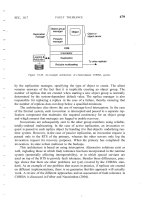
Figure 37.8 is the histogram of 1000 sample variances, each calculated using three observations drawn
from a normal distribution with
σ

2
= 25. The average of the simulated sample variances was 25.3, with
30 values above 100 and 190 values of five or less. This is the range of variation in for sample size n = 3.
A formal comparison of the equality of two sample variances uses the F statistic. Comparing two samples
variances, each estimated with three degrees of freedom, would use the upper 5% value of F
3,3
= 9.28. If
the ratio of the larger to the smaller of two variances is less than this F value, the two variances would be
considered equal. For F
3,3
= 9.28, this would include variances from 25/9.28 = 2.7 to 25(9.28) = 232.
This shows that the variance of repeat observations in a calibration experiment will be quite variable
due to random experimental error. If triplicate observations in a calibration experiment did have true
constant variance
σ

2
= 25, replicates at one concentration level could have s
2
= 3, and at another level
(not necessarily a higher concentration) the variance could be s
2
= 200. Therefore, our interest is not in
‘‘unchanging” variance, but rather in the pattern of change over the range of x or y. If change from one
level of y to another is random, the variances are probably just reflecting random sampling error. If the
variance increases in proportion to one of the variables, weighted least squares should be used.

Making the slopes in Figure 37.7 integer values was justified by saying that the variance is estimated
with low precision when there are only three replicates. Box (personal communication) has shown that
the percent error in the variance is % error = 100/ , where
ν
is the degrees of freedom. From this,
about 200 observations of y would be needed to estimate the variance with an error of 5%.
Comments
Nonconstant variance may occur in a variety of situations. It is common in calibration data because they
cover a wide range of concentration, and also because certain measurement errors tend to be multiplicative
instead of additive.
Using unweighted least squares when there is nonconstant variance will distort all calculated t statistics,
confidence intervals, and prediction intervals. It will lead to wrong decisions about the form of the
calibration model and which parameters should be included in the model, and give biased estimates of
analyte concentrations.
The appropriate weights can be determined from the data if replicate measurements have been made
at some settings of x. These should be true replicates and not merely multiple measurements on the same
standard solution.
If there is no replication, one may falsely assume that the variance is constant when it is not. If you
suspect nonconstant variance, based on prior experience or knowledge about an instrument, apply reasonable
weights. Any reasonable weighting is likely to be better than none.
FIGURE 37.8 Distribution of 1000 simulated sample variances, each calculated using three observations drawn at random
from a normal distribution with
σ
2
= 25. The average of the 1000 simulated values is 25.3, with 30 variances above 100
and 190 variances of five or less.
0 25 50 75 100 125 150
0
100
200

Simulated Sample Variance,
s
2
Frequency
s
i
2
2
ν
L1592_frame_C37.fm Page 334 Tuesday, December 18, 2001 3:20 PM
© 2002 By CRC Press LLC
One reason analysts often make many measurements at low concentrations is to use the calibration
data to calculate the limit of detection for the measurement process. If this is to be done, proper weighting
is critical (Zorn et al., 1997 and 1999).
References
Currie, L. A. (1984). “Chemometrics and Analytical Chemistry,” in Chemometrics: Mathematics and Statistics
in Chemistry, NATO ASI Series C, 138, 115–146.
Danzer, K. and L. A. Currie (1998). “Guidelines for Calibration in Analytical Chemistry,” Pure Appl. Chem.,
70, 993–1014.
Gibbons, R. D. (1994). Statistical Methods for Groundwater Monitoring, New York, John Wiley.
Draper, N. R. and H. Smith, (1998). Applied Regression Analysis, 3rd ed., New York, John Wiley.
Otto, M. (1999). Chemometrics, Weinheim, Germany, Wiley-VCH.
Zorn, M. E., R. D. Gibbons, and W. C. Sonzogni (1999). ‘‘Evaluation of Approximate Methods for Calculating
the Limit of Detection and Limit of Quantitation,” Envir. Sci. & Tech., 33(13), 2291–2295.
Zorn, M. E., R. D. Gibbons, and W. C. Sonzogni (1997). “Weighted Least Squares Approach to Calculating
Limits of Detection and Quantification by Modeling Variability as a Function of Concentration,” Anal.
Chem., 69(15), 3069–3075.
Exercises
37.1 ICP Calibration. Fit the ICP calibration data for iron (Fe) below using weights that are inversely
proportional to the square of the peak intensity (I).

37.2 Nitrate Calibration I. For the case study nitrate data (Table 37.1), plot the residuals obtained
by fitting a cubic calibration curve using unweighted regession.
37.3 Nitrate Calibration II. For the case study nitrate data (Table 37.1), compare the results of
fitting the calibration curve using weights 1/x
2
with those obtained using 1/s
2
and 1/y
2
.
37.4 Chloride Calibration. The following table gives triplicate calibration peaks for HPLC mea-
surement of chloride. Determine appropriate weights and fit the calibration curve. Plot the
residuals to check the adequacy of the calibration model.
Standard Fe Conc. (mg/L) 0 50 100 200
Peak Intensity (I) 0.029 109.752 217.758 415.347
Chloride (mg/L) Peak 1 Peak 2 Peak 3
0.2 1112 895 1109
0.5 1892 1806 1796
0.7 3242 3162 3191
1.0 4519 4583 4483
2.0 9168 9159 9146
3.5 15,915 16,042 15,935
5.0 23,485 23,335 23,293
10.0 49,166 50,135 49,439
17.5 92,682 93,288 92,407
25.0 137,021 140,137 139,938
50.0 318,984 321,468 319,527
75.0 505,542 509,773 511,877
100.0 700,231 696,155 699,516
Source: Greg Zelinka, Madison Metropolitan Sewerage District.

L1592_frame_C37.fm Page 335 Tuesday, December 18, 2001 3:20 PM
© 2002 By CRC Press LLC
37.5 BOD Parameter Estimation. The data below are duplicate measurements of the BOD of fresh
bovine manure. Use weighted nonlinear least squares to estimate the parameters in the model
η
=
θ
1
(1 − exp (−
θ
2
t).
Day 13571015
BOD (mg/L) 11,320 20,730 28,000 32,000 35,200 33,000
11,720 22,320 29,600 33,600 32,000 36,600
Source: Marske, D. M. and L. B. Polkowski (1972). J. WPCF, 44, 1987–1992.
L1592_frame_C37.fm Page 336 Tuesday, December 18, 2001 3:20 PM
© 2002 By CRC Press LLC

38

Empirical Model Building by Linear Regression

KEY WORDS

all possible regressions, analysis of variance, coefficient of determination, confidence
interval, diagnostic checking, empirical models,

F

test, least squares, linear regression, overfitting, par-
simonious model, polynomial, regression sum of squares, residual plot, residual sum of squares, sedimen-
tation, solids removal, standard error,

t

statistic, total sum of squares.

Empirical models are widely used in engineering. Sometimes the model is a straight line; sometimes a
mathematical French curve — a smooth interpolating function — is needed. Regression provides the
means for selecting the complexity of the French curve that can be supported by the available data.
Regression begins with the specification of a model to be fitted. One goal is to find a

parsimonious
model

— an adequate model with the fewest possible terms. Sometimes the proposed model turns out
to be too simple and we need to augment it with additional terms. The much more common case,
however, is to start with more terms than are needed or justified. This is called

overfitting

. Overfitting
is harmful because the prediction error of the model is proportional to the number of parameters in
the model.
A fitted model is always checked for inadequacies. The statistical output of regression programs is
somewhat helpful in doing this, but a more satisfying and useful approach is to make diagnostic plots
of the residuals. As a minimum, the residuals should be plotted against the predicted values of the fitted
model. Plots of residuals against the independent variables are also useful. This chapter illustrates how
this diagnosis is used to decide whether terms should be added or dropped to improve a model. If a tentative

model is modified, it is refitted and rechecked. The model builder thus works iteratively toward the
simplest adequate model.

A Model of Sedimentation

Sedimentation removes solid particles from a liquid by allowing them to settle under quiescent conditions.
An ideal sedimentation process can be created in the laboratory in the form of a batch column. The column
is filled with the suspension (turbid river water, industrial wastewater, or sewage) and samples are taken over
time from sampling ports located at several depths along the column. The measure of sedimentation efficiency
will be solids concentrations (or fraction of solids removed), which will be measured as a function of
time and depth.
The data come from a quiescent batch settling test. At the beginning of the test, the concentration is
uniform over the depth of the test settling column. The mass of solids in the column initially is

M



=

C

0

ZA

, where

C

0

is the initial concentration (g/m

3

),

Z

is the water depth in the settling column (m), and

A

is the cross-sectional area of the column (m

2

). This is shown in the left-hand panel of Figure 38.1.
After settling has progressed for time

t

, the concentration near the bottom of the column has increased
relative to the concentration at the top to give a solids concentration profile that is a function of depth
at any time

t

. The mass of solids remaining above depth

z

is

M



=



A

∫

C

(

z

,

t

)

dz

. The total mass of solids
in the column is still

M



=



C

0

ZA

. This is shown in the right-hand panel of Figure 38.1.

L1592_frame_C38 Page 337 Tuesday, December 18, 2001 3:21 PM
© 2002 By CRC Press LLC

The fraction of solids removed in a settling tank at any depth

z

, that has a detention time

t

, is estimated
as:

This integral could be calculated graphically (Camp, 1946) or an approximating polynomial can be
derived for the concentration curve and the fraction of solids removed (

R

) can be calculated algebraically.
Suppose, for example, that:

C

(

z

,

t

)

=

167

−

2.74

t



+

11.9

z



−

0.08

zt



+

0.014

t

2

is a satisfactory empirical model and we want to use this model to predict the removal that will be achieved
with 60-min detention time, for a depth of 8 ft and an initial concentration of 500 mg/L. The solids concen-
tration profile as a function of depth at

t



=

60 min is:

C

(

z

,

t

)

=

167

−

2.74(60)

+

11.9

z



−

0.08

z

(60)

+

0.014(60)

2



=

53.0

+

7.1

z


This is integrated over depth (

Z



=

8 ft) to give the fraction of solids that are expected to be removed:

The model building problem is to determine the form of the polynomial function and to estimate the
coefficients of the terms in the function.

Method: Linear Regression

Suppose the correct model for the process is

η



=

f

(

β

,

x

) and the observations are

y

i



=



f

(

β

,

x

)

+



e

i

, where
the

e

i

are random errors. There may be several parameters (

β

) and several independent variables (

x

).
According to the least squares criterion, the best estimates of the

β

’s minimize the sum of the squared
residuals:

where the summation is over all observations.

FIGURE 38.1

Solids concentration as a function of depth at time. The initial condition (

t



=

0) is shown on the left. The
condition at time

t

is shown on the right.
0
Z
z
d

z
C(
z
,
t
)0
0
0
Z



C


0
Solids
profile at
settling
time t = 0
Solids profile at
settling time t
Mass of solids
M = C
0
ZA
Mass of solids
M = A” C(
z, t
) dz

Depth
Rz, t()
AZC
0
A∫
0
z
Cz, t()zd–
AZC
0

1
1
ZC
0

Cz, t()zd
0
z
∫
–==
Rz 8, t 60==()1
1
8500()

53.0 7.1z+()zd
z=0
z=8
∫
–=

1
1
8500()

53 8() 3.55 8
2
()+()– 0.84==
minimize S
β
() y
i
η
i
–()
2
∑
=

L1592_frame_C38 Page 338 Tuesday, December 18, 2001 3:21 PM
© 2002 By CRC Press LLC

The minimum sum of squares is called the residual sum of squares, RSS. The residual mean square
(RMS) is the residual sum of squares divided by its degrees of freedom. RMS = RSS /(n − p), where n =
number of observations and p = number of parameters estimated.
Case Study: Solution
A column settling test was done on a suspension with initial concentration of 560 mg/L. Samples were
taken at depths of 2, 4, and 6 ft (measured from the water surface) at times 20, 40, 60, and 120 min;
the data are in Table 38.1. The simplest possible model is:
C(z, t) =
β

0
+
β
1
t
The most complicated model that might be needed is a full quadratic function of time and depth:
C(z, t) =
β
0
+
β
1
t +
β
2
t
2
+
β
3
z +
β
4
z
2
+
β
5
zt
We can start the model building process with either of these and add or drop terms as needed.

Fitting the simplest possible model involving time and depth gives:

which has R
2
= 0.844 and residual mean square = 355.82. R
2
, the coefficient of determination, is the
percentage of the total variation in the data that is accounted for by fitting the model (Chapter 39).
Figure 38.2a shows the diagnostic residual plots for the model. The residuals plotted against the
predicted values are not random. This suggests an inadequacy in the model, but it does not tell us how
TABLE 38.1
Data from a Laboratory Settling Column Test
Suspended Solids Concentration at Time t (min)
Depth (ft) 20 40 60 120
2 135 90 75 48
4 170 110 90 53
6 180 126 96 60
FIGURE 38.2 (a) Residuals plotted against the predicted suspended solids concentrations are not random. (b) Residuals
plotted against settling time suggest that a quadratic term is needed in the model.
y
ˆ
132.3 7.12z 0.97t–+=
L1592_frame_C38 Page 339 Tuesday, December 18, 2001 3:21 PM
© 2002 By CRC Press LLC
the model might be improved. The pattern of the residuals plotted against time (Figure 38.2b) suggests
that adding a t
2
term may be helpful. This was done to obtain:

which has R

2
= 0.97 and residual mean square = 81.5. A diagnostic plot of the residuals (Figure 38.3)
reveals no inadequacies. Similar plots of residuals against the independent variables also support the
model. This model is adequate to describe the data.
The most complicated model, which has six parameters, is:
The model contains quadratic terms for time and depth and the interaction of depth and time (zt). The
analysis of variance for this model is given in Table 38.2. This information is produced by computer
programs that do linear regression. For now we do not need to know how to calculate this, but we should
understand how it is interpreted.
Across the top, SS is sum of squares and df = degrees of freedom associated with a sum of squares
quantity. MS is mean square, where MS = SS/df. The sum of squares due to regression is the regression
sum of squares (RegSS): RegSS = 20,255.5. The sum of squares due to residuals is the residual sum of
squares (RSS); RSS = 308.8. The total sum of squares, or Total SS, is:
Total SS = RegSS + RSS
Also:
The residual sum of squares (RSS) is the minimum sum of squares that results from estimating the parameters
by least squares. It is the variation that is not explained by fitting the model. If the model is correct, the RSS
is the variation in the data due to random measurement error. For this model, RSS = 308.8. The residual
mean square is the RSS divided by the degrees of freedom of the residual sum of squares. For RSS, the
degrees of freedom is df = n − p, where n is the number of observations and p is the number of parameters
in the fitted model. Thus, RMS = RSS /(n − p). The residual sum of squares (RSS = 308.8) and the
TABLE 38.2
Analysis of Variance for the Six-Parameter Settling
Linear Model
Due to df SS MS = SS/df
Regression (Reg SS) 5 20255.5 4051.1
Residuals (RSS) 6 308.8 51.5
Total (Total SS) 11 20564.2
FIGURE 38.3 Plot of residuals against the predicted values of the regression model = 185.97 + 7.125t + 0.014t
2

− 3.057z.
•
•
•
•
•
•
•
•
•
•
•
•
Predicted SS Values
Residuals
10
-10
0
160
40 80 120
200
y
ˆ
y
ˆ
186.0 7.12z 3.06t– 0.0143t
2
++=
y
ˆ

152 20.9z 2.74t– 1.13z
2
– 0.0143t
2
0.080zt––+=
Total SS y
i
y–()
2
∑
=
L1592_frame_C38 Page 340 Tuesday, December 18, 2001 3:21 PM
© 2002 By CRC Press LLC
residual mean square (RMS = 308.8/6 = 51.5) are the key statistics in comparing this model with simpler
models.
The regression sum of squares (RegSS) shows how much of the total variation (i.e., how much of the
Total SS) has been explained by the fitted equation. For this model, RegSS = 20,255.5.
The coefficient of determination, commonly denoted as R
2
, is the regression sum of squares expressed
as a fraction of the total sum of squares. For the complete six-parameter model (Model A in Table 38.3),
R
2
= (20256/20564) = 0.985, so it can be said that this model accounts for 98.5% of the total variation
in the data.
It is natural to be fascinated by high R
2
values and this tempts us to think that the goal of model building
is to make R
2

as high as possible. Obviously, this can be done by putting more high-order terms into a
model, but it should be equally obvious that this does not necessarily improve the predictions that will
be made using the model. Increasing R
2
is the wrong goal. Instead of worrying about R
2
values, we
should seek the simplest adequate model.
Selecting the “Best” Regression Model
The “best” model is the one that adequately describes the data with the fewest parameters. Table 38.3
summarizes parameter estimates, the coefficient of determination R
2
, and the regression sum of squares
for all eight possible linear models. The total sum of squares, of course, is the same in all eight cases
because it depends on the data and not on the form of the model. Standard errors [SE] and t ratios (in
parentheses) are given for the complete model, Model A.
One approach is to examine the t ratio for each parameter. Roughly speaking, if a parameter’s t ratio
is less than 2.5, the true value of the parameter could be zero and that term could be dropped from the
equation.
Another approach is to examine the confidence intervals of the estimated parameters. If this interval
includes zero, the variable associated with the parameter can be dropped from the model. For example,
in Model A, the coefficient of z
2
is b
3
= −1.13 with standard error = 1.1 and 95% confidence interval
[ −3.88 to +1.62]. This confidence interval includes zero, indicating that the true value of b
3
is very likely
to be zero, and therefore the term z

2
can be tentatively dropped from the model. Fitting the simplified
model (without z
2
) gives Model B in Table 38.3.
The standard error [SE] is the number in brackets. The half-width of the 95% confidence interval is
a multiple of the standard error of the estimated value. The multiplier is a t statistic that depends on the
selected level of confidence and the degrees of freedom. This multiplier is not the same value as the
t ratio given in Table 38.3. Roughly speaking, if the degrees of freedom are large (n − p ≥ 20), the half-
width of the confidence interval is about 2SE for a 95% confidence interval. If the degrees of freedom
are small (n − p < 10), the multiplier will be in the range of 2.3SE to 3.0SE.
TABLE 38.3
Summary of All Possible Regressions for the Settling Test Model
Coefficient of the Term
Decrease
Model b
0
b
1
zb
2
tb
3
z
2
b
4
t
2
b

5
tz R
2
RegSS in RegSS
A 152 20.9 −2.74 −1.13 0.014 −0.08 0.985 20256
(t ratio) (2.3) (8.3) (1.0) (7.0) (2.4)
[SE] [9.1] [0.33] [1.1] [0.002] [0.03]
B 167 11.9 −2.74 0.014 −0.08 0.982 20202 54
C 171 16.1 −3.06 −1.13 0.014 0.971 19966 289
D 186 7.1 −3.06 0.143 0.968 19912 343
E 98 20.9 −0.65 −1.13 −0.08 0.864 17705 2550
F 113 11.9 −0.65 −0.08 0.858 17651 2605
G 117 16.1 −0.97 −1.13 0.849 17416 2840
H 132 7.1 −0.97 0.844 17362 2894
Note: () indicates t ratios of the estimated parameters. [] indicates standard errors of the estimated parameters.
L1592_frame_C38 Page 341 Tuesday, December 18, 2001 3:21 PM
© 2002 By CRC Press LLC
After modifying a model by adding, or in this case dropping, a term, an additional test should be
made to compare the regression sum of squares of the two models. Details of this test are given in
texts on regression analysis (Draper and Smith, 1998) and in Chapter 40. Here, the test is illustrated
by example.
The regression sum of squares for the complete model (Model A) is 20,256. Dropping the z
2
term to
get Model B reduced the regression sum of squares by only 54. We need to consider that a reduction
of 54 in the regression sum of squares may not be a statistically significant difference.
The reduction in the regression sum of squares due to dropping z
2
can be thought of as a variance
associated with the z

2
term. If this variance is small compared to the variance of the pure experimental
error, then the term z
2
contributes no real information and it should be dropped from the model. In
contrast, if the variance associated with the z
2
term is large relative to the pure error variance, the term
should remain in the model.
There were no repeated measurements in this experiment, so an independent estimate of the variance
due to pure error variance cannot be computed. The best that can be done under the circumstances is to
use the residual mean square of the complete model as an estimate of the pure error variance. The residual
mean square for the complete model (Model A) is 51.5. This is compared with the difference in regression
sum of squares of the two models; the difference in regression sum of squares between Models A and B
is 54. The ratio of the variance due to z
2
and the pure error variance is F = 54/51.5 = 1.05. This value is
compared against the upper 5% point of the F distribution (1, 6 degrees of freedom). The degrees of
freedom are 1 for the numerator (1 degree of freedom for the one parameter that was dropped from the
model) and 6 for the denominator (the mean residual sum of squares). From Table C in the appendix,
F
1,6
= 5.99. Because 1.05 < 5.99, we conclude that removing the z
2
term does not result in a significant
reduction in the regression sum of squares. Therefore, the z
2
term is not needed in the model.
The test used above is valid to compare any two of the models that have one less parameter than
Model A. To compare Models A and E, notice that omitting t

2
decreases the regression sum of squares
by 20256 − 17705 = 2551. The F statistic is 2551/51.5 = 49.5. Because 49.5 >> 5.99 (the upper 95%
point of the F distribution with 1 and 6 degrees of freedom), this change is significant and t
2
needs to be
included in the model.
The test is modified slightly to compare Models A and D because Model D has two less terms than
Model A. The decrease of 343 in the regression sum of squares results from dropping to terms (z
2
and zt).
The F statistic is now computed using 343/2 in the numerator and 51.5 in the denominator: F =
(343/2)/51.5 = 3.33. The upper 95% point of the appropriate reference distribution is F = 5.14, which
has 2 degrees of freedom for the numerator and 6 degrees of freedom for the denominator. Because F
for the model is less than the reference F (F = 3.33 < 5.14), the terms z
2
and zt are not needed.
Model D is as good as Model A. Model D is the simplest adequate model:

This is the same model that was obtained by starting with the simplest possible model and adding terms
to make up for inadequacies.
Comments
The model building process uses regression to estimate the parameters, followed by diagnosis to decide
whether the model should be modified by adding or dropping terms. The goal is not to maximize R
2
,
because this puts unneeded high-order terms into the polynomial model. The best model should have
the fewest possible parameters because this will minimize the prediction error of the model.
One approach to finding the simplest adequate model is to start with a simple tentative model and use
diagnostic checks, such as residuals plots, for guidance. The alternate approach is to start by overfitting

the data with a highly parameterized model and to then find appropriate simplifications. Each time a
Model D y
ˆ
186 7.12t 3.06z– 0.143t
2
++=
L1592_frame_C38 Page 342 Tuesday, December 18, 2001 3:21 PM
© 2002 By CRC Press LLC
term is added or deleted from the model, a check is made on whether the difference in the regression sum
of squares of the two models is large enough to justify modification of the model.
References
Berthouex, P. M. and D. K. Stevens (1982). “Computer Analysis of Settling Data,” J. Envr. Engr. Div., ASCE,
108, 1065–1069.
Camp, T. R. (1946). “Sedimentation and Design of Settling Tanks,” Trans. Am. Soc. Civil Engr., 3, 895–936.
Draper, N. R. and H. Smith (1998). Applied Regression Analysis, 3rd ed., New York, John Wiley.
Exercises
38.1 Settling Test. Find a polynomial model that describes the following data. The initial suspended
solids concentration was 560 mg/L. There are duplicate measurements at each time and depth.
38.2 Solid Waste Fuel Value. Exercise 3.5 includes a table that relates solid waste composition to
the fuel value. The fuel value was calculated from the Dulong model, which uses elemental
composition instead of the percentages of paper, food, metal, and plastic. Develop a model
to relate the percentages of paper, food, metals, glass, and plastic to the Dulong estimates of
fuel value. One proposed model is E(Btu/lb) = 23 Food + 82.8 Paper + 160 Plastic. Compare
your model to this.
38.3 Final Clarifier. An activated sludge final clarifier was operated at various levels of overflow
rate (OFR) to evaluate the effect of overflow rate (OFR), feed rate, hydraulic detention time,
and feed slurry concentration on effluent total suspended solids (TSS) and underflow solids
concentration. The temperature was always in the range of 18.5 to 21°C. Runs 11–12, 13–14,
and 15–16 are duplicates, so the pure experimental error can be estimated. (a) Construct a
polynomial model to predict effluent TSS. (b) Construct a polynomial model to predict

underflow solids concentration. (c) Are underflow solids and effluent TSS related?
Susp. Solids Conc. at Time t (min)
Depth (ft) 20 40 60 120
2 135 90 75 48
140 100 66 40
4 170 110 90 53
165 117 88 46
6 180 126 96 60
187 121 90 63
Feed Detention Feed Effluent
OFR Rate Time Slurry Underflow TSS
Run (m/d) (m/d) (h) (kg/m
3
) (kg/m
3
) (mg/L)
1 11.1 30.0 2.4 6.32 11.36 3.5
2 11.1 30.0 1.2 6.05 10.04 4.4
3 11.1 23.3 2.4 7.05 13.44 3.9
4 11.1 23.3 1.2 6.72 13.06 4.8
5 16.7 30.0 2.4 5.58 12.88 3.8
6 16.7 30.0 1.2 5.59 13.11 5.2
7 16.7 23.3 2.4 6.20 19.04 4.0
8 16.7 23.3 1.2 6.35 21.39 4.5
9 13.3 33.3 1.8 5.67 9.63 5.4
L1592_frame_C38 Page 343 Tuesday, December 18, 2001 3:21 PM
© 2002 By CRC Press LLC
38.4 Final Clarification. The influence of three factors on clarification of activated sludge effluent
was investigated in 36 runs. Three runs failed because of overloading. The factors were solids
retention time = SRT, hydraulic retention time = HRT, and overflow rate (OFR). Interpret the

data.
10 13.3 20.0 1.8 7.43 20.55 3.0
11 13.3 26.7 3.0 6.06 12.20 3.7
12 13.3 26.7 3.0 6.14 12.56 3.6
13 13.3 26.7 0.6 6.36 11.94 6.9
14 13.3 26.7 0.6 5.40 10.57 6.9
15 13.3 26.7 1.8 6.18 11.80 5.0
16 13.3 26.7 1.8 6.26 12.12 4.0
Source: Adapted from Deitz J. D. and T. M. Keinath, J. WPCF, 56, 344–350.
(Original values have been rounded.)
SRT HRT OFR Eff TSS SRT HRT OFR Eff TSS
Run (d) (h) (m/d) (mg/L) Run (d) (h) (m/d) (mg/L)
1 8 12 32.6 48 19 5 12 16.4 18
2 8 12 32.6 60 20 5 12 8.2 15
3 8 12 24.5 55 21 5 8 40.8 47
4 8 12 16.4 36 22 5 8 24.5 41
5 8 12 8.2 45 23 5 8 8.2 57
6 8 8 57.0 64 24 5 4 40.8 39
7 8 8 40.8 55 25 5 4 24.5 41
8 8 8 24.5 30 26 5 4 8.2 43
9 8 8 8.2 16 27 2 12 16.4 19
10 8 8 8.2 45 28 2 12 16.4 36
11 8 4 57.0 37 29 2 12 8.2 23
12 8 4 40.8 21 30 2 8 40.8 26
13 8 4 40.8 14 31 2 8 40.8 15
14 8 4 24.5 4 32 2 8 24.5 17
15 8 4 8.2 11 33 2 8 8.2 14
16 5 12 32.6 20 34 2 4 40.8 39
17 5 12 24.5 28 35 2 4 24.5 43
18 5 12 24.5 12 36 2 4 8.2 48

Source: Cashion B. S. and T. M. Keinath, J. WPCF, 55, 1331–1338.
L1592_frame_C38 Page 344 Tuesday, December 18, 2001 3:21 PM
© 2002 By CRC Press LLC

39

The Coefficient of Determination, R

2

KEY WORDS

coefficient of determination, coefficient of multiple correlation, confidence interval,

F

ratio, hapenstance data, lack of fit, linear regression, nested model, null model, prediction interval, pure
error,

R

2

, repeats, replication, regression, regression sum of squares, residual sum of squares, spurious
correlation.

Regression analysis is so easy to do that one of the best-known statistics is the coefficient of determi-
nation,

R

2

. Anderson-Sprecher (1994) calls it “…a measure many statistician’s love to hate.”
Every scientist knows that

R

2

is the

coefficient of determination

and

R

2

is that proportion of the total
variability in the dependent variable that is explained by the regression equation. This is so seductively
simple that we often assume that a high

R

2

signifies a useful regression equation and that a low

R

2

signifies the opposite. We may even assume further that high

R

2

indicates that the observed relation
between independent and dependent variables is true and can be used to predict new conditions.
Life is not this simple. Some examples will help us understand what

R

2

really reveals about how well
the model fits the data and what important information can be overlooked if too much reliance is placed
on the interpretation of

R

2

.

What Does “Explained” Mean?

Caution is recommended in interpreting the phrase “

R

2

explains the variation in the dependent variable.”

R

2

is the proportion of variation in a variable

Y

that can be accounted for by fitting

Y

to a particular
model instead of viewing the variable in isolation.

R

2

does not explain anything in the sense that “Aha!
Now we know why the response indicated by

y

behaves the way we have observed in this set of data.”
If the data are from a well-designed controlled experiment, with proper replication and randomization,
it is reasonable to infer that an significant association of the variation in

y

with variation in the level of

x

is a causal effect of

x

. If the data had been observational, what Box (1966) calls

happenstance data,

there is a high risk of a causal interpretation being wrong. With observational data there can be many
reasons for associations among variables, only one of which is causality.
A value of

R

2

is not just a rescaled measure of variation. It is a comparison between two models. One
of the models is usually referred to as

the model

. The other model —

the null model

— is usually never
mentioned. The null model (

y



=



β

0

) provides the reference for comparison. This model describes a
horizontal line at the level of the mean of the

y

values, which is the simplest possible model that could
be fitted to any set of data.
• The model (

y



=



β

0



+



β

1

x



+

β

2

x



+



…
+



e

i

) has residual sum of squares
• The null model (

y



=

β

0



+



e

i

) has residual sum of squares
The comparison of the residual sums of squares (RSS) defines:

∑ (y
i
y
ˆ
)–
2
RSS
model
.=
∑ (y

i
y)–
2
RSS
null model
.=
R
2
1
RSS
model
RSS
null model
–=

L1592_frame_C39 Page 345 Tuesday, December 18, 2001 3:22 PM
© 2002 By CRC Press LLC

This shows that

R

2

is a model comparison and that large

R

2

measures only how much the model improves
the null model. It does not indicate how good the model is in any absolute sense. Consequently, the
common belief that a large

R

2

demonstrates model adequacy is sometimes wrong.
The definition of

R

2

also shows that comparisons are made only between

nested models

. The concept
of proportionate reduction in variation is untrustworthy unless one model is a special case of the other.
This means that

R

2

cannot be used to compare models with an intercept with models that have no
intercept:

y



=



β

0

is not a reduction of the model

y



=



β

1

x

. It is a reduction of

y



=



β

0



+



β

1

x

and

y

=



β

0



+

β

1

x



+



β

2

x

2

.

A High

R

2

Does Not Assure a Valid Relation

Figure 39.1 shows a regression with

R

2



=

0.746, which is statistically significant at almost the 1% level
of confidence (a 1% chance of concluding significance when there is no true relation). This might be
impressive until one knows the source of the data.

X

is the first six digits of pi, and

Y

is the first six
Fibonocci numbers. There is no true relation between

x

and

y

. The linear regression equation has no
predictive value (the seventh digit of pi does not predict the seventh Fibonocci number).
Anscombe (1973) published a famous and fascinating example of how

R

2

and other statistics that are
routinely computed in regression analysis can fail to reveal the important features of the data. Table 39.1

FIGURE 39.1

An example of nonsense in regression.

X

is
the first six digits of pi and

Y

is the first six Fibonocci
numbers. R

2

is high although there is no actual relation
between

x

and

y

.

TABLE 39.1

Anscombe’s Four Data Sets

A

B

C

D

xyxyxyxy

10.0 8.04 10.0 9.14 10.0 7.46 8.0 6.58
8.0 6.95 8.0 8.14 8.0 6.77 8.0 5.76
13.0 7.58 13.0 8.74 13.0 12.74 8.0 7.71
9.0 8.81 9.0 8.77 9.0 7.11 8.0 8.84
11.0 8.33 11.0 9.26 11.0 7.81 8.0 8.47
14.0 9.96 14.0 8.10 14.0 8.84 8.0 7.04
6.0 7.24 6.0 6.13 6.0 6.08 8.0 5.25
4.0 4.26 4.0 3.10 4.0 5.39 19.0 12.50
12.0 10.84 12.0 9.13 12.0 8.15 8.0 5.56
7.0 4.82 7.0 7.26 7.0 6.42 8.0 7.91
5.0 5.68 5.0 4.74 5.0 5.73 8.0 6.89

Note:

Each data set has

n



=

11, mean of mean of equation
of the regression line

y

=

3.0

+ 0.5x, standard error of estimate of
the slope = 0.118 (t statistic = 4.24, regression sum of squares
(corrected for mean) = 110.0, residual sum of squares = 13.75,
correlation coefficient r = 0.82 and R
2
= 0.67).
Source: Anscombe, F. J. (1973). Am. Stat., 27, 17–21.
X
Y
Y = 0.31 + 0.79X
R
2
= 0.746
0
2
4
6
8
10
1086420
x 9.0,= y 7.5,=
L1592_frame_C39 Page 346 Tuesday, December 18, 2001 3:22 PM
© 2002 By CRC Press LLC
gives Anscombe’s four data sets. Each data set has n = 11, fitted regression line

standard error of estimate of the slope = 0.118 (t statistic = 4.24), regression sum of
squares (corrected for mean) = 110.0, residual sum of squares = 13.75, correlation coefficient = 0.82,
and R
2
= 0.67. All four data sets appear to be described equally well by exactly the same linear model,
at least until the data are plotted (or until the residuals are examined). Figure 39.2 shows how vividly
they differ. The example is a persuasive argument for always plotting the data.

A Low R
2
Does Not Mean the Model is Useless
Hahn (1973) explains that the chances are one in ten of getting R
2
as high as 0.9756 in fitting a simple
linear regression equation to the relation between an independent variable x and a normally distributed
variable y based on only three observations, even if x and y are totally unrelated. On the other hand,
with 100 observations, a value of R
2
= 0.07 is sufficient to establish statistical significance at the 1% level.
Table 39.2 lists the values of R
2
required to establish statistical significance for a simple linear regression
equation. Table 39.2 applies only for the straight-line model y =
β
0
+
β
1
x + e; for multi-variable regression
models, statistical significance must be determined by other means. This tabulation gives values at the

10, 5, and 1% significance levels. These correspond, respectively, to the situations where one is ready to
take one chance in 10, one chance in 20, and one chance in 100 of incorrectly concluding there is evidence
of a statistically significant linear regression when, in fact, x and y are unrelated.
A Significant R
2
Doesn’t Mean the Model is Useful
Practical significance and statistical significance are not equivalent. Statistical significance and impor-
tance are not equivalent. A regression based on a modest and unimportant true relationship may be
established as statistically significant if a sufficiently large number of observations are available. On the
other hand, with a small sample it may be difficult to obtain statistical evidence of a strong relation.
It generally is good news if we find R
2
large and also statistically significant, but it does not assure a
useful equation, especially if the equation is to be used for prediction. One reason is that the coefficient
of determination is not expressed on the same scale as the dependent variable. A particular equation
FIGURE 39.2 Plot of Anscombe’s four data sets which all have R
2
= 0.67 and identical results from simple linear regression
analysis (data from Anscombe 1973).
y
y
(a) R
2
= 0.67 (b) R
2
= 0.67
(c) R
2
= 0.67 (d) R
2

= 0.67
0
5
10
15
0
5
10
15
2015105020151050
x
x
x 9.0, y 7.5,==
y
ˆ
30.5x,+=
L1592_frame_C39 Page 347 Tuesday, December 18, 2001 3:22 PM
© 2002 By CRC Press LLC
may explain a large proportion of the variability in the dependent variable, and thus have a high R
2
, yet
unexplained variability may be too large for useful prediction. It is not possible to tell from the magnitude
of R
2
how accurate the predictions will be.
The Magnitude of R
2
Depends on the Range of Variation in X
The value of R
2

decreases with a decrease in the range of variation of the independent variable, other
things being equal, and assuming the correct model is being fitted to the data. Figure 39.3 (upper
left-hand panel) shows a set of 50 data points that has R
2
= 0.77. Suppose, however, that the range
of x that could be investigated is only from 14 to 16 (for example, because a process is carefully
constrained within narrow operating limits) and the available data are those shown in the upper right-
hand panel of Figure 39.3. The underlying relationship is the same, and the measurement error in
each observation is the same, but R
2
is now only 0.12. This dramatic reduction in R
2
occurs mainly
because the range of x is restricted and not because the number of observations is reduced. This is
shown by the two lower panels. Fifteen points (the same number as found in the range of x = 14 to
16), located at x = 10, 15, and 20, give R
2
= 0.88. Just 10 points, at x = 10 and 20, gives an even
larger value, R
2
= 0.93.
These examples show that a large value of R
2
might reflect the fact that data were collected over
an unrealistically large range of the independent variable x. This can happen, especially when x is
time. Conversely, a small value might be due to a limited range of x, such as when x is carefully
controlled by a process operator. In this case, x is constrained to a narrow range because it is known
to be highly important, yet this importance will not be revealed by doing regression on typical data
from the process.
Linear calibration curves always have a very high R

2
, usually 0.99 and above. One reason is that the
x variable covers a wide range (see Chapter 36.)

TABLE 39.2
Values of R
2
Required to Establish Statistical
Significance of a Simple Linear Regression
Equation for Various Sample Sizes
Sample Size
Statistical Significance Level
n 10% 5% 1%
3 0.98 0.99 0.99
4 0.81 0.90 0.98
5 0.65 0.77 0.92
6 0.53 0.66 0.84
8 0.39 0.50 0.70
10 0.30 0.40 0.59
12 0.25 0.33 0.50
15 0.19 0.26 0.41
20 0.14 0.20 0.31
25 0.11 0.16 0.26
30 0.09 0.13 0.22
40 0.07 0.10 0.16
50 0.05 0.08 0.13
100 0.03 0.04 0.07
Source: Hahn, G. J. (1973). Chemtech, October,
pp. 609– 611.
L1592_frame_C39 Page 348 Tuesday, December 18, 2001 3:22 PM

© 2002 By CRC Press LLC
The Effect of Repeated Runs on R
2
If regression is used to fit a model to n settings of x, it is possible for a model with n parameters to fit
the data exactly, giving R
2
= 1. This kind of overfitting is not recommended but it is mathematically
possible. On the other hand, if repeat measurements are made at some or all of the n settings of the
independent variables, a perfect fit will not be possible. This assumes, of course, that the repeat measure-
ments are not identical.
The data in Figure 39.4 are given in Table 39.3. The fitted model is The relevant
statistics are presented in Table 39.4. The fraction of the variation explained by the regression is R
2
=
581.12/697.5 = 0.833. The residual sum of squares (RSS) is divided into the pure error sum of squares
(SS
PE
), which is calculated from the repeated measurements, and the lack-of-fit sum of squares (SS
LOF
).
That is:
RSS = SS
PE
+ SS
LOF
FIGURE 39.3 The full data set of 50 observations (upper-left panel) has R
2
= 0.77. The other three panels show how R
2
depends on the range of variation in the independent variable.

FIGURE 39.4 Linear regression with repeated observations. The regression sum of squares is 581.12. The residual sum of
squares (RSS = 116.38) is divided into pure error sum of squares (SS
PE
= 112.34) and lack-of-fit sum of squares (SS
LOF
=
4.04). R
2
= 0.833, which explains 99% of the amount of residual error that can be explained.
•
•
•
•
•
•
•
•
•
•
•
•
•
•
•
•
•
•
•
•
•

•
•
•
•
•
•
•
•
•
•
•
•
•
•
•
•
•
•
•
•
•
•
•
•
•
•
•
•
•
•

•
•
•
•
•
•
•
•
•
•
•
•
•
•
•
•
•
•
•
•
•
•
•
•
•
•
•
•
•
•

•
•
•
R
2
= 0.77
R
2
= 0.88
R
2
= 0.12
R
2
= 0.93
30
20
10
30
20
10
y
y
10
10
20 2015 15
x
x
3020100
0

25
50
x
y
^

y
= 15.4 + 0.97
x
y
ˆ
15.45 0.97x.+=
L1592_frame_C39 Page 349 Tuesday, December 18, 2001 3:22 PM
© 2002 By CRC Press LLC
Suppose now that there had been only five observations (that is, no repeated measurements) and
furthermore that the five values of y fell at the average of the repeated values in Figure 39.4. Now the
fitted model would be exactly the same: but the R
2
value would be 0.993. This is
because the variance due to the repeats has been removed.
The maximum possible value for R
2
when there are repeat measurements is:

The pure error SS does not change when terms are added or removed from the model in an effort to
improve the fit. For our example:

The actual R
2
= 581.12/697.5 = 0.83. Therefore, the regression has explained 100(0.833/0.839) = 99%

of the amount of variation that can be explained by the model.
A Note on Lack-Of-Fit
If repeat measurements are available, a lack-of-fit (LOF) test can be done. The lack-of-fit mean square
is compared with the pure error mean square If the model gives an
adequate fit, these two sums of squares should be of the same magnitude. This is checked by comparing the
ratio against the F statistic with the appropriate degrees of freedom. Using the values in Table 39.4
gives = 1.35/11.23 = 0.12. The F statistic for a 95% confidence test with three degrees of freedom
to measure lack of fit and ten degrees of freedom to measure the pure error is F
3,10
= 3.71. Because
= 0.12 is less than F
3,10
= 3.71, there is no evidence of lack-of-fit. For this lack-of-fit test to be
valid, true repeats are needed.
TABLE 39.3
Linear Regression with Repeated
Observations
xy
1
y
2
y
3

5 17.5 22.4 19.2
12 30.4 28.4 25.1
14 30.1 25.8 31.1
19 36.6 31.3 34.0
24 38.9 43.2 32.7
TABLE 39.4

Analysis of Variance of the Regression with Repeat Observations Shown in Figure 39.4
Source df Sum of Sq. Mean Sq. F Ratio Comments
Regression 1 581.12 581.12 64.91
Residual 13 116.38 8.952 = s
2
Lack of fit (LOF) 3 4.04 1.35 0.12 =
Pure error (PE) 10 112.34 11.23 =
Total (Corrected) 14 697.50
s
L
2
s
e
2
y
ˆ
15.45 0.97x+=
max R
2
Total SS (corrected) Pure error SS–
Total SS (corrected)

=
max R
2
697.5 112.3–
697.5

0.839==
s

L
2
SS
LOF
/df
LOF
=
s
e
2
SS
PE
/df
PE
.=
s
L
2
/s
e
2
s
L
2
/s
e
2
s
L
2

/s
e
2
L1592_frame_C39 Page 350 Tuesday, December 18, 2001 3:22 PM
© 2002 By CRC Press LLC
A Note on Description vs. Prediction
Is the regression useful? We have seen that a high R
2
does not guarantee that a regression has meaning.
Likewise, a low R
2
may indicate a statistically significant relationship between two variables although
the regression is not explaining much of the variation. Even less does statistically significant mean that
the regression will predict future observations with much accuracy. “In order for the fitted equation to
be regarded as a satisfactory predictor, the observed F ratio (regression mean square/residual mean
square) should exceed not merely the selected percentage point of the F distribution, but several times
the selected percentage point. How many times depends essentially on how great a ratio (prediction
range/error of prediction) is specified” (Box and Wetz, 1973). Draper and Smith (1998) offer this rule-
of-thumb: unless the observed F for overall regression exceeds the chosen test percentage point by at
least a factor of four, and preferably more, the regression is unlikely to be of practical value for prediction
purposes. The regression in Figure 39.4 has an F ratio of 581.12/8.952 = 64.91 and would have some
practical predictive value.
Other Ways to Examine a Model
If R
2
does not tell all that is needed about how well a model fits the data and how good the model may
be for prediction, what else could be examined?
Graphics reveal information in data (Tufte 1983): always examine the data and the proposed model
graphically. How sad if this advice was forgotten in a rush to compute some statistic like R
2

.
A more useful single measure of the prediction capability of a model (including a k-variate regression
model) is the standard error of the estimate. The standard error of the estimate is computed from the
variance of the predicted value and it indicates the precision with which the model estimates the
value of the dependent variable. This statistic is used to compute intervals that have the following
meanings (Hahn, 1973).
• The confidence interval for the dependent variable is an interval that one expects, with a
specified level of confidence, to contain the average value of the dependent variable at a set
of specified values for the independent variables.
• A prediction interval for the dependent variable is an interval that one expects, with a specified
probability, to contain a single future value of the dependent variable from the sampled
population at a set of specified values of the independent variables.
• A confidence interval around a parameter in a model (i.e., a regression coefficient) is an
interval that one expects, with a specified degree of confidence, to contain the true regression
coefficient.
Confidence intervals for parameter estimates and prediction intervals for the dependent variable are
discussed in Chapters 34 and 35. The exact method of obtaining these intervals is explained in Draper
and Smith (1998). They are computed by most statistics software packages.
Comments
Widely used methods have the potential to be frequently misused. Linear regression, the most widely
used statistical method, can be misused or misinterpreted if one relies too much on R
2
as a characterization
of how well a model fits.
R
2
is a measure of the proportion of variation in y that is accounted for by fitting y to a particular linear
model instead of describing the data by calculating the mean (a horizontal straight line). High R
2
does not

prove that a model is correct or useful. A low R
2
may indicate a statistically significant relation between two
variables although the regression has no practical predictive value. Replication dramatically improves the
predictive error of a model, and it makes possible a formal lack-of-fit test, but it reduces the R
2
of the model.
(y
ˆ
)
L1592_frame_C39 Page 351 Tuesday, December 18, 2001 3:22 PM
© 2002 By CRC Press LLC
Totally spurious correlations, often with high R
2
values, can arise when unrelated variables are
combined. Two examples of particular interest to environmental engineers are presented by Sherwood
(1974) and Rowe (1974). Both emphasize graphical analysis to stimulate and support any regression
analysis. Rowe discusses the particular dangers that arise when sets of variables are combined to create
new variables such as dimensional numbers (Froude number, etc.). Benson (1965) points out the same
kinds of dangers in the context of hydraulics and hydrology.
References
Anderson-Sprecher, R. (1994). “Model Comparison and R
2
,” Am. Stat., 48(2), 113–116.
Anscombe, F. J. (1973). “Graphs in Statistical Analysis,” Am. Stat., 27, 17–21.
Benson, M. A. (1965). “Spurious Correlation in Hydraulics and Hydrology,” J. Hydraulics Div., ASCE, 91,
HY4, 35–45.
Box, G. E. P. (1966). “The Use and Abuse of Regression,” Technometrics, 8, 625–629.
Box, G. E. P. and J. Wetz (1973). “Criteria for Judging Accuracy of Estimation by an Approximating Response
Function,” Madison, WI, University of Wisconsin Statistics Department, Tech. Rep. No. 9.

Draper, N. R. and H. Smith (1998). Applied Regression Analysis, 3rd ed., New York, John Wiley.
Hahn, G. J. (1973). “The Coefficient of Determination Exposed,” Chemtech, October, pp. 609–611.
Rowe, P. N. (1974). “Correlating Data,” Chemtech, January, pp. 9–14.
Sherwood, T. K. (1974). “The Treatment and Mistreatment of Data,” Chemtech, December, pp. 736–738.
Tufte, E. R. (1983). The Visual Display of Quantitative Information, Cheshire, CT, Graphics Press.
Exercises
39.1 COD Calibration. The ten pairs of readings below were obtained to calibrate a UV spectro-
photometer to measure chemical oxygen demand (COD) in wastewater.
(a) Fit a linear model to the data and obtain the R
2
value. (b) Discuss the meaning of R
2
in
the context of this calibration problem. (c) Exercise 36.3 contains a larger calibration data
set for the same instrument. (d) Fit the model to the larger sample and compare the values
of R
2
. Will the calibration curve with the highest R
2
best predict the COD concentration?
Explain why or why not.
39.2 Stream pH. The data below are n = 200 monthly pH readings on a stream that cover a period of
almost 20 years. The data read from left to right. The fitted regression model is = 7.1435 −
0.0003776t; R
2
= 0.042. The confidence interval of the slope is [−0.00063, −0.000013]. Why
is R
2
so low? Is the regression statistically significant? Is stream pH decreasing? What is the
practical value of the model?

COD (mg/L) 60 90 100 130 195 250 300 375 500 600
UV Absorbance 0.30 0.35 0.45 0.48 0.95 1.30 1.60 1.80 2.3 2.55
7.0 7.2 7.2 7.3 7.2 7.2 7.2 7.2 7.0 7.1 7.3 7.1 7.1 7.1 7.2 7.3 7.2 7.3 7.2 7.2
7.1 7.4 7.1 6.8 7.3 7.3 7.0 7.0 6.9 7.2 7.2 7.3 7.0 7.0 7.1 7.1 7.0 7.2 7.2 7.2
7.2 7.1 7.2 7.0 7.0 7.2 7.1 7.1 7.2 7.2 7.2 7.0 7.1 7.1 7.2 7.1 7.2 7.0 7.1 7.2
7.1 7.0 7.1 7.4 7.2 7.2 7.2 7.2 7.1 7.0 7.2 7.0 6.9 7.2 7.0 7.0 7.1 7.0 6.9 6.9
7.0 7.0 7.2 6.9 7.4 7.0 6.9 7.0 7.1 7.0 7.2 7.2 7.0 7.0 7.1 7.1 7.0 7.2 7.2 7.0
7.0 7.2 7.1 7.1 7.1 7.0 7.0 7.0 7.1 7.3 7.1 7.2 7.2 7.2 7.1 7.2 7.2 7.1 7.1 7.1
7.2 6.8 7.2 7.2 7.0 7.1 7.1 7.2 7.0 7.1 7.1 7.1 7.0 7.2 7.1 7.1 7.3 6.9 7.2 7.2
7.1 7.1 7.0 7.0 7.1 7.1 7.0 7.0 7.0 7.1 7.0 7.1 7.1 7.2 7.2 7.1 7.0 7.0 7.2 7.2
7.0 7.1 7.2 7.1 7.1 7.0 7.1 7.0 7.2 7.1 7.1 7.1 7.2 7.1 7.0 7.1 7.2 7.2 7.1 7.2
7.0 7.1 7.0 7.1 7.0 6.9 6.9 7.2 7.1 7.2 7.1 7.1 7.0 7.0 6.9 7.1 6.8 7.1 7.0 7.0
y
ˆ
L1592_frame_C39 Page 352 Tuesday, December 18, 2001 3:22 PM
© 2002 By CRC Press LLC
39.3 Replication. Fit a straight-line calibration model to y
1
and then fit the straight line to the three
replicate measures of y. Suppose a colleague in another lab had the y
1
data only and you had
all three replicates. Who will have the higher R
2
and who will have the best fitted calibration
curve? Compare the values of R
2
obtained. Estimate the pure error variance. How much of
the variation in y has been explained by the model?
39.4 Range of Data. Fit a straight-line calibration model to the first 10 observations in the Exercise

36.3 data set, that is for COD between 60 and 195 mg/L. Then fit the straight line to the full
data set (COD from 60 to 675 mg/L). Interpret the change in R
2
for the two cases.
xy
1
y
2
y
3
2 0.0 1.7 2.0
5 4.0 2.0 4.5
8 5.1 4.1 5.8
12 8.1 8.9 8.4
15 9.2 8.3 8.8
18 11.3 9.5 10.9
20 11.7 10.7 10.4
L1592_frame_C39 Page 353 Tuesday, December 18, 2001 3:22 PM
© 2002 By CRC Press LLC

40

Regression Analysis with Categorical Variables

KEY WORDS

acid rain,

pH

, categorical variable, F test, indicator variable, east squares, linear model,
regression, dummy variable, qualitative variables, regression sum of squares,

t

-ratio, weak acidity.

Qualitative variables can be used as explanatory variables in regression models. A typical case would be
when several sets of data are similar except that each set was measured by a different chemist (or different
instrument or laboratory), or each set comes from a different location, or each set was measured on a
different day. The qualitative variables — chemist, location, or day — typically take on discrete values
(i.e., chemist Smith or chemist Jones). For convenience, they are usually represented numerically by a
combination of zeros and ones to signify an observation’s membership in a category; hence the name

categorical variables

.
One task in the analysis of such data is to determine whether the same model structure and parameter
values hold for each data set. One way to do this would be to fit the proposed model to each individual
data set and then try to assess the similarities and differences in the goodness of fit. Another way would
be to fit the proposed model to all the data as though they were one data set instead of several, assuming
that each data set has the same pattern, and then to look for inadequacies in the fitted model.
Neither of these approaches is as attractive as using categorical variables to create a collective data
set that can be fitted to a single model while retaining the distinction between the individual data sets.
This technique allows the model structure and the model parameters to be evaluated using statistical
methods like those discussed in the previous chapter.

Case Study: Acidification of a Stream During Storms

Cosby Creek, in the southern Appalachian Mountains, was monitored during three storms to study how

pH and other measures of acidification were affected by the rainfall in that region. Samples were taken
every 30 min and 19 characteristics of the stream water chemistry were measured (Meinert et al., 1982).
Weak acidity (WA) and pH will be examined in this case study.
Figure 40.1 shows 17 observations for storm 1, 14 for storm 2, and 13 for storm 3, giving a total of
44 observations. If the data are analyzed without distinguishing between storms one might consider
models of the form pH

=



β

0



+



β

1

WA



+

β

2

WA

2

or pH

=



θ

3



+

(

θ

1

−



θ

3

)exp(

−θ

2

WA

). Each storm might be
described by pH

=



β

0

+



β

1

WA

, but storm 3 does not have the same slope and intercept as storms 1 and
2, and storms 1 and 2 might be different as well. This can be checked by using categorical variables to
estimate a different slope and intercept for each storm.

Method: Regression with Categorical Variables

Suppose that a model needs to include an effect due to the category (storm event, farm plot, treatment,
truckload, operator, laboratory, etc.) from which the data came. This effect is included in the model in
the form of categorical variables (also called

dummy

or

indicator variables

). In general

m



−

1 categorical
variables are needed to specify

m

categories.

L1592_frame_C40 Page 355 Tuesday, December 18, 2001 3:24 PM
© 2002 By CRC Press LLC

Begin by considering data from a single category. The quantitative predictor variable is

x

1

which can
predict the independent variable

y

1

using the linear model:

where

β

0

and

β

1

are parameters to be estimated by least squares.
If there are data from two categories (e.g., data produced at two different laboratories), one approach
would be to model the two sets of data separately as:

and

and then to compare the estimated intercepts (

α

0

and

β

0

) and the estimated slopes (

α

1

and

β

1

) using
confidence intervals or

t

-tests.
A second, and often better, method is to simultaneously fit a single augmented model to all the data.
To construct this model, define a categorical variable

Z

as follows:
The augmented model is:

With some rearrangement:

In this last form the regression is done as though there are three independent variables,

x

,

Z

, and

Zx

.
The vectors of

Z

and

Zx

have to be created from the categorical variables defined above. The four
parameters

α

0

,

β

0

,

α

1

, and

β

1

are estimated by linear regression.
A model for each category can be obtained by substituting the defined values. For the first category,

Z



=

0 and:


FIGURE 40.1

The relation of pH and weak acidity data of Cosby Creek after three storms.

Z = 0 if the data are in the first category

Z



=

1 if the data are in the second category
7006005004003002001000
5.
6.
6.
7.
pH
5
0
5
0
Weak Acidity (µg/L)
y
1i
β
0
β
1
x
1i
e

i
++=
y
1i
α
0
α
1
x
1i
e
i
++=
y
2i
β
0
β
1
x
2i
e
i
++=
y
i
α
0
α
1

x
i
Z
β
0
β
1
x
i
+()e
i
++ +=
y
i
α
0
β
0
Z
α
1
x
i
β
1
Zx
i
e
i
++++=

y
i
α
0
α
1
x
i
e
i
++=

L1592_frame_C40 Page 356 Tuesday, December 18, 2001 3:24 PM
© 2002 By CRC Press LLC

For the second category,

Z



=

1 and:

The regression might estimate either

β

0

or

β

1

as zero, or both as zero. If

β

0



=

0, the two lines have the
same intercept. If

β

1



=

0, the two lines have the same slope. If both

β

1

and

β

0

equal zero, a single straight
line fits all the data. Figure 40.2 shows the four possible outcomes. Figure 40.3 shows the particular
case where the slopes are equal and the intercepts are different.
If simplification seems indicated, a simplified version is fitted to the data. We show later how the full
model and simplified model are compared to check whether the simplification is justified.
To deal with three categories, two categorical variables are defined:
This implies

Z

1



=

0 and

Z

2



=

0 for category 3.
The model is:

The parameters with subscript 0 estimate the intercept and those with subscript 1 estimate the slopes.
This can be rearranged to give:

The six parameters are estimated by fitting the original independent variable

x

i

plus the four created
variables

Z

1
, Z
2
, Z
1
x
i

, and Z
2
x
i
.
Any of the parameters might be estimated as zero by the regression analysis. A couple of examples
explain how the simpler models can be identified. In the simplest possible case, the regression would
FIGURE 40.2 Four possible models to fit a straight line to data in two categories.
FIGURE 40.3 Model with two categories having different intercepts but equal slopes.
Category 1: Z
1
= 1 and Z
2
= 0
Category 2: Z
1
= 0 and Z
2
= 1
Intercepts
Different
Intercepts
Equal
y
i
=(
α
0
+
β

0
) +(
α
1
+
β
1
)
x
i
+
e
i
y
i
=
α
0
+(
α
1
+
β
1
)
x
i
+
e
i

y
i
=(
α
0
+
β
0
) +
α
1
x
i

+
e
i

y
i
=
α
0
+
α
1
x
i
+
e

i
Slopes Diffferent Slopes Equal

α
0
+
β
0
α
α
0
β
0
slope = α
1
for both lines
Complete model
y=
(
α
0
+
β
0
)+(
α
1
+
β
1

)
x
+
e
Category 2:
y =
(
α
0
+
β
0
)+
α
1
x
+
e
Category 1:
y =
α
0
+
α
1
x
+
e
1
α

1
y
i
α
0
β
0
+()
α
1
β
1
+()x
i
e
i
++=
y
i
α
0
α
1
x
i
+()Z
1
β
0
β

1
x
i
+()Z
2
γ
0
γ
1
x
i
+()e
i
+++=
y
i
α
0
β
0
Z
1
+
γ
0
Z
2
α
1
x

i
+
β
1
Z
1
x
i
γ
1
Z
2
x
i
e
i
++++=
L1592_frame_C40 Page 357 Tuesday, December 18, 2001 3:24 PM
© 2002 By CRC Press LLC
estimate
β
0
= 0,
γ

0
= 0,
β
1
= 0, and

γ
1
= 0 and the same slope (
α
1
) and intercept (
α

0
) would apply to
all three categories. The fitted simplified model is .
If the intercepts are different for the three categories but the slopes are the same, the regression would
estimate
β
1
= 0 and
γ
1
= 0 and the model becomes:
For category 1:
For category 2:
For category 3:
Case Study: Solution
The model under consideration allows a different slope and intercept for each storm. Two dummy variables
are needed:
Z
1
= 1 for storm 1 and zero otherwise
Z
2

= 1 for storm 2 and zero otherwise
The model is:
pH =
α
0
+
α
1
WA + Z
1
(
β
0
+
β
1
WA ) + Z
2
(
γ
0
+
γ
1
WA )
where the
α
’s,
β
’s, and

γ
’s are estimated by regression. The model can be rewritten as:
pH =
α
0
+
β
0
Z
1
+
γ
0
Z
2
+
α
1
WA +
β
1
Z
1
WA +
γ
1
Z
2
WA
The dummy variables are incorporated into the model by creating the new variables Z

1
WA and Z
2
WA.
Table 40.1 shows how this is done.
Fitting the full six-parameter model gives:
Model A: pH = 5.77 − 0.00008WA + 0.998Z
1
+ 1.65Z
2
− 0.005Z
1
WA − 0.008Z
2
WA
(t-ratios) (0.11) (2.14) (3.51) (3.63) (4.90)
which is also shown as Model A in Table 40.2 (top row). The numerical coefficients are the least squares
estimates of the parameters. The small numbers in parentheses beneath the coefficients are the t-ratios
for the parameter values. Terms with t < 2 are candidates for elimination from the model because they
are almost certainly not significant.
The term WA appears insignificant. Dropping this term and refitting the simplified model gives Model
B, in which all coefficients are significant:
Model B: pH = 5.82 + 0.95Z
1
+ 1.60Z
2
− 0.005Z
1
WA − 0.008Z
2

WA
(t-ratios) (6.01) (9.47) (4.35) (5.54)
[95% conf. interval] [0.63 to 1.27] [1.26 to 1.94] [−0.007 to −0.002] [−0.01 to −0.005]
The regression sum of squares, listed in Table 40.2, is the same for Model A and for Model B (Reg SS =
4.278). Dropping the WA term caused no decrease in the regression sum of squares. Model B is equivalent
to Model A.
Is any further simplification possible? Notice that the 95% confidence intervals overlap for the terms
−0.005 Z
1
WA and –0.008 Z
2
WA. Therefore, the coefficients of these two terms might be the same. To
check this, fit Model C, which has the same slope but different intercepts for storms 1 and 2. This is
y
i
α
0
α
1
x
i
+ e
i
+=
y
i
α
0
β
0

Z
1
γ
0
Z
2
++()
α
1
x
i
e
i
++=
y
i
α
0
β
0
Z
1
+()
α
1
x
i
e
i
++=

y
i
α
0
γ
0
Z
2
+()
α
1
x
i
e
i
++=
y
i
α
0
α
1
x
i
e
i
++=
L1592_frame_C40 Page 358 Tuesday, December 18, 2001 3:24 PM
© 2002 By CRC Press LLC
done by combining columns Z

1
WA and Z
2
WA to form the two columns on the right-hand side of
Table 40.1. Call this new variable Z
3
WA. Z
3
= 1 for storms 1 and 2, and 0 for storm 3.
The fitted model is:
Model C: pH = 5.82 + 1.11Z
1
+ 1.38Z
2
− 0.0057Z
3
WA
(t-ratios) (8.43) (12.19) (6.68)
TABLE 40.1
Weak Acidity (WA), pH, and Categorical Variables for Three Storms
Storm WA Z
1
Z
2
Z
1
WA Z
2
WA pH Z
3

Z
3
WA
1 190 1 0 190 0 5.96 1 190
1 110 1 0 110 0 6.08 1 110
1 150 1 0 150 0 5.93 1 150
1 170 1 0 170 0 5.99 1 170
1 170 1 0 170 0 6.01 1 170
1 170 1 0 170 0 5.97 1 170
1 200 1 0 200 0 5.88 1 200
1 140 1 0 140 0 6.06 1 140
1 140 1 0 140 0 6.06 1 140
1 160 1 0 160 0 6.03 1 160
1 140 1 0 140 0 6.02 1 140
1 110 1 0 110 0 6.17 1 110
1 110 1 0 110 0 6.31 1 110
1 120 1 0 120 0 6.27 1 120
1 110 1 0 110 0 6.42 1 110
1 110 1 0 110 0 6.28 1 110
1 110 1 0 110 0 6.43 1 110
2 140 0 1 0 140 6.33 1 140
2 140 0 1 0 140 6.43 1 140
2 120 0 1 0 120 6.37 1 120
2 190 0 1 0 190 6.09 1 190
2 120 0 1 0 120 6.32 1 120
2 110 0 1 0 110 6.37 1 110
2 110 0 1 0 110 6.73 1 110
2 100 0 1 0 100 6.89 1 100
2 100 0 1 0 100 6.87 1 100
2 120 0 1 0 120 6.30 1 120

2 120 0 1 0 120 6.52 1 120
2 100 0 1 0 100 6.39 1 100
2 80 0 1 0 80 6.87 1 80
2 100 0 1 0 100 6.85 1 100
3 580 0 0 0 0 5.82 0 0
3 640 0 0 0 0 5.94 0 0
3 500 0 0 0 0 5.73 0 0
3 530 0 0 0 0 5.91 0 0
3 670 0 0 0 0 5.87 0 0
3 670 0 0 0 0 5.80 0 0
3 640 0 0 0 0 5.80 0 0
3 640 0 0 0 0 5.78 0 0
3 560 0 0 0 0 5.78 0 0
3 590 0 0 0 0 5.73 0 0
3 640 0 0 0 0 5.63 0 0
3 590 0 0 0 0 5.79 0 0
3 600 0 0 0 0 6.02 0 0
Note: The two right-hand columns are used to fit the simplified model.
Source: Meinert, D. L., S. A. Miller, R. J. Ruane, and H. Olem (1982). “A Review of Water Quality
Data in Acid Sensitive Watersheds in the Tennessee Valley,” Rep. No. TVA.ONR/WR-82/10, TVA,
Chattanooga, TN.
L1592_frame_C40 Page 359 Tuesday, December 18, 2001 3:24 PM