A Guide to Microsofl Excel 2002 for Scientists and Engineers phần 7 ppt

Modelling
I
I87
_
1
.eo
0
1M)
200
300
400
500
_
Vdum
pr
wanh
I
.66
1.72
1.76

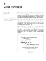
Figure
9.13
2.* The radioactive decay sequence shown
in
Equation
9.7
occurs
in
nuclear reactors. When the reactor
is

operating the neutron
flux destroys the
I
and Xe. When it is shut down there
is
a
residual concentration of each isotope. Because the half-life of
1'"
is smaller than that of Xe'js, the concentration of the latter
reaches a maximum and then decays to zero. The reactor
cannot be restarted until the XeI3' is well passed its maximum.
The equations governing the production of the
two
isotopes
are
:
>xe13'
9.*3hrs
>
cs'35
1135
6.68hrs
411
-
=-k*[I]
dt
where [Xe] and
[I]
denote concentrations, and
k,,

and
k,
are
the decay constants. The decay constant
k
of a radioisotope is
related to its half-life
A
by
k/z
=
ln2.
Your task is to model this system and show how the
concentration of Xe varies with time for given initial
concentrations
of
I
and Xe. We will approximate the first
equation
in
Equation
9.6
as
A[I]
=
-k,[I]At,
giving
[I],
=
[]lo(

1
-kt),
where
[IlO
is the initial concentration of
1"'
when
the reactor is shut down, and
[I],
is the concentration after time
t.
What
condition is needed
for
this approximation
to
be
justified? The equation for [Xe]
is
treated similarly. Construct
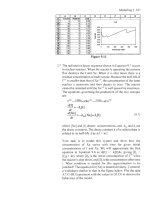
a worksheet similar to that in the figure below. Plot the data
A7:C
108.
Experiment with the values
in
D3:D5
to observe the
behaviour of the model.
188
A

Guide
to
Microsoft
Excel
2002
for Scientists and Engineers
3.*
C!
I
100)
46.001
0.01491
0.15651
1011
46501
0
0141
I
0
15131
Because microprocessors have limited memory, their programs
must be kept very small. The algorithm shown below has been
suggested as a quick way to generate
two
cycles
of
a sine
wave. The value
of
Quick(?)

is
an approximation to sin(90);
Quick(n)
approximates sin(90-5.625*(n-
1)).
Start with q(1)
=
128 and d(1)
=
-1
Quick(1)
=
q(1)/128
For
n
=
2
to
129
=
d(n-1)
-
1
=
d(n-1)
+
1
=
q(n-
1)

+
d(n)
when q(n)
>=
0
when q(n)
<
0
d(n)
Quick(n)
=
q(n)/l28
Next
n
Your
task
is
to compare the results from this algorithm with
the true sine values. The figure below shows how
to
start the
worksheet. Carefully consider the entries needed in row
3
which will allow you to copy that row down to row
130.
Plot
the data
in
the
Quick

and
Sine
columns against that
in
the
n
column.
10
Solving
Equations
Concepts
Roots
A:
Finding
In
this section we examine methods of finding roots of non-linear
equations such as polynomial
(32
-
72
-
22x
+
40
=
0)
and
transcendental (exp(-x)
-
sin(x)

=
0).
If
the equation
is
written as
Ax) then a
root
of the equation is a value of
x
such thatJx)
=
0.
The value of x
is
sometimes called the zero
of
the function. Some
equations may be solved analytically. The quadratic formula, for
example, is used to find the roots of a quadratic equation. With
other equations the analytical method may be very complex or not
exist at all.
In
these cases we may use numerical methods to find
approximate roots. One should also remember the usefulness of
graphing a function to determine the number and values
of
its
roots.
Microsoft Excel includes

two
tools (Goal Seek and Solver) for
finding roots.
A
discussion
of
the algorithms used by these tools is
beyond the scope of this book but if you are familiar with the
bisection or the Newton-Raphson method you will have some
appreciation of how they work. We show
in
the first exercise how
the bisection, or interval halving, method may be implemented on
a
worksheet. It is left as an exercise to the interested reader to
develop a worksheet implementation of the Newton-Raphson
method. Subsequent exercises use Goal Seek and Solver to find
approximate roots.
Exercise
1
:
The
Bisection
Method
In
Figure 10.
I
the values of
F(a)
and

F(b)
lie on opposite sides
of
the x-axis. Therefore there is
a
root of
F(x)
lying between
a
and
b.
Let
m
be the midpoint of the interval
a
to
b.
Since
F(m)
has the
opposite sign of
F(b),
this root lies between
m
and
b.
By
halving
the interval we have a more accurate idea of the value of the root.
Looking at the function G(x) we see that the root lies between

a
and
m.
So
we must use the values
m
and
a
to
find
the next
approximation. Of course we may repeat this halving over and
over; successive iterations giving smaller intervals
-
the
a
and
b
values will converge.
I90
A
Guide
to
Microsoft
Excel
2002for
Scientists and Engineers
Figure
10.1
This allows us to develop an algorithm

for
finding a root
ofAx):
Start with values
of
a
and b
such
thatf(a) and
Ab)
have
opposite signs
Loop
until the required accuracy
is
achieved
Find the midpoint
M
=
(a
+
b)/2
IfAm)
andAb) have opposite
signs
Else
End
if
End loop.
give

a
the
value
of
m
give
b
the value
of
m
f(x)
1
.o
0.8
0.6
0.4
0.2
0.0
-0.2
-0.4
-0.6
-0.8
-1
.o
exp(-x)
-
sin(x)
J
I
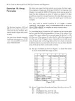
Figure

10.2
Solving
Equations
I91
To
demonstrate how we may implement this algorithm
in
Excel,
we shall find the roots of the function exp(-x)
-
sin(x). Figure
10.2
shows a plot of this function for values
of
x
from
0
to
4.
Clearly, this equation has one root at approximately
0.6
and
another near
3. Our task is to find more exactly what these values
are. In subsequent exercises we use
Goal
Seek and Solver to find
the roots of this equation and compare their results with those
obtained in this exercise.
(a) Open a new workbook. On Sheet1 enter the text shown

in
A1:F3
of Figure
10.3.
(b) On row
4
enter:
A4:
0.5
The first
a
value
B4:
1
The first
b
value
C4:
=(A4+B4)/2
Compute the midpoint
m
D4:
=EXP(-A4)
-
SIN(A4)
The value
offla)
E4:
=EXP(-B4)
-

SIN(B4)
The value offlb)
F4:
=EXP(-C4)
-
SIN(C4)
The value ofAm)
To save time, the formula
in
D4
may be copied
to
E4:F4
by
dragging
D4s
fill
handle to the right
two
cells.
Row
4
sets the initial conditions. Next we compute the next
interval. In Row
5
we compute the first approximation.
(c) In
A5
enter the formula
=

IF(SlGN(F4)<>SlGN(E4), C4, A4).
This compares the signs ofAm) andAb). If they differ then cell
A5
(the new
a
value)
is
given the value
of
m of the first
approximation. Otherwise the cell retains the old
a
value.
Figure
10.3
192
A
Guide
lo
Microsoft
Excel
2002
for Scientists and Engineers
(d)
In
B5 enter the formula
=IF(SIGN(F4)<>SlGN(E4),84,C4).
This keeps the old value for
b
when the signs ofAm) andAb)

differ but uses the
old
m
value for the next b when the signs
are the same. The values
in
A5
and
A4
are equal when
a
was
not replaced by
m;
in
which case the new
b
value
is
the
m
value from the first approximation. Otherwise the previous b
value is used.
To compute successive iterations we copy row
5
down the sheet.
But for how may rows? Recalling that each interation halves the
interval, we note that 20 iterations will reduce the interval by
a
factor of

2*'
or about a millionfold. Surely this will be more than
enough!
(e) Copy C4:F4 down to row 24.
In
Figure
10.3
rows 10:20 have
been hidden to make the figure smaller.
In
row 4Ab) andAm) have the same sign,
so
the new
b
value
in
row
5
is the previous
m
value. The same occurs when going from
row
5
to row
6.
But nowAb) and Am) have the same sign,
so
in
row
7

the
m
value
is
passed to
a.
On row
24
with x
=
0.588533,
the function evaluates to
8
x
1
O-'
which
is
acceptably close to
0.
The values
in
the
A
and
B
columns
are not changing very much at this point. You may wish to copy
row
24

down to row
50.
At this point the function evaluates to
approximately
1
x
so
we are at the limit of precision of Excel.
You will not see any changes
in
the
a
and b values unless you
widen the columns or use a formula to display the difference
in
successive values.
(f)
From Figure
10.2
we know there is a root near
3.
Replace the
initial values of
a
and
b in
line
4
to find this second root. It
does not matter much if you use

3
and
4,
or
3
and
3.5.
Why is
this?
(g)
Save the workbook as
CHAP
1O.XLS.
Finding
Roots
with
How would you answer this question: For what value ofx does the
function
3x3
-
10x2
-
x
+
1
evaluate to
1
OO?
You could find the
answer by trial and error. Enter some value for x

in
A
1
and
in
B
1
enter the formula
=
3*AIA3
-
1
O*AlA2
-
AI
+
1.
Now vary AI until
the desired result
is
obtained. This is exactly what Excel's Goal
Seek does but with the help of a mathematical algorithm.
Goal
Seek
Solving Equations
193
When
Goal Seek
is
running you specify three things: (i) that

B
1
is
the cell of interest
-
the
Set cell,
(ii) that the value you require is
100
-
the
To
value,
and (iii) that
A1
is the cell whose value is to be
changed- the
By
changing
cell.
Goal Seek changes the value
of
A
1
until it finds avalue which gives the formula
in
B1 the value close
to 100.
If
you had specified a value

of
0
rather than
100,
then the
value
in
AI
would be one of the roots of the functions
in
B
I.
Goal Seek is a very easy tool to use but it has its limitations.
In
the
next section ofthis chapter we see that Solver is far more powerful.
Exercise
2:
A
Simple
In
this exercise we will
find
the roots
of
2x’
-
5x
-
12

=
0
using
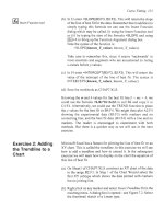
Goal Seek. The plot
in
Figure 10.4
will
help us understand which
solution Microsoft Excel finds.
If
we make an initial guess of
0,
Quadratic Equation
denoted by point
GI
on the plot, then Goal Seek will find the root
with value
-
I
.5
at the point
R,.
Goal Seek ‘explores’ the point
GI
and determines that the function moves closer to zero as
x
becomes
more negative. Conversely, if the initial guess is 3 (the point
G2),
Goal Seek finds the root with the value 4.

h
y
=
2x2-
5x
-
12
15
10
5
0
-5
-1
0
-1
5
Figure
10.4
(a) Open the workbook CHAP1
0.XLS
and move to Sheet2. Start
with a worksheet similar to that
in
Figure 10.5.
In
B3 type the
formula
=2*A3*A3-5*A3-12.
Copy this to cell B4.
(b) Make

63
the active cell. On
the
menu bar, click
Tools
followed by Goal Seek. Complete the Goal Seek dialog box as
shown
in
Figure
10.6.
You may type
A3
in
the
By
changing
cell
box, or, with the box selected, click
on
the
A3
cell.
In
the
second case, Excel enters the value
$A$3.
Now click the
OK
button.
194

A
Guide to Microsoft Excel
2002
for Scientists
and
Engineers
A
B
C
I
1
ITosolve2x2-5x-12
=O
I
3
4
121
Root
I
Function
1
0
-1
2
3
-9
Figure
10.5
Figure
10.6

(c) The Goal Seek Status dialog box appears; see Figure
10.7.
This reports that our target value was
0
and Goal Seek has
obtained a value of -3.3424E
-
05.
This is very close to zero
so
we will click the
OK
button. Goal Seek has changed the
value of A3 to
-1.5.
With this value ofx the function evaluates
essentially to zero (-3.3
x
so
this value is a root of the
function.
Figure
10.7
(d) Make
B4
the active cell and repeat steps (b) and (c) to find the
next root. On my PC the value in
A4
becomes
4

and
B4
has a
value of
-2.513
-
06.
Save the workbook
CHAP1
0.XLS.
Accuracy
Why does the worksheet report values for the function that are not
exactly zero when it uses
x
values that appear exactly correct for
Solving
Equations
I95
the roots? If you widen the
A
column the answer is that Goal Seek
did not find the
exact
value
-1.5
and
4.
My
PC
gave the values

-1.49999696 145665
and
3.99999977326809,
respectively. Goal
Seek uses an iterative algorithm
to
get closer and closer to the
solution. It therefore needs to stop at some point.
In
our case it
stopped just short
of
the exact solutions. Type the values
-1.5
and
4
into cells
A3
and
A4,
respectively. The two function values will
now be exactly
0.
The problem with using Goal Seek
or
Solver to find the roots of
quadratic equations
is
that you have to provide an initial guess. If
the equation has one real root you will generally have no problem

finding it. When there are two roots, your initial guesses may all
converge to the same solution. This frustration can be avoided by
using a worksheet based on the quadratic formula as demonstrated
in
an earlier chapter.
Exercise
3:
Solving a
If we have only one quadratic equation to solve it
is
probably more
efficient to use the quadratic formula manually rather than setting
up a worksheet. Cubic equations are a different matter. Here the
tasks of trying various guesses is worth the effort. When finding
the solution to
a
cubic equation is part of a physical problem, we
may know the approximate value
of
the root
in
which we are
interested or there may be only one real root. Either of these cases
will simplify the
task
of making the initial guess.
Cubic Equation
In
this exercise we will set up a worksheet that may be used to
solve a cubic equation. We shall used

named
cells. You should
recall from an earlier exercise that if we attempt to use ‘c’ as a
name Microsoft Excel replaces this by ‘c-’.
(a) Open
CHAP1O.XLS
and on Sheet3 enter the values of all the
cells except
E4
to
E6
as shown
in
Figure
10.8.
(b)
Select the range
A4:B7
and use@.ertlPJamelCreate to name the
cells
B4:B7
as ‘a’, ‘b’, ‘c-’, and ‘d’, respectively. Note that
with the values shown
in
B4:B7,
we have set the worksheet to
solve the equation
2x’
+
x2

-
246x
+
360
=
0.
When you typed
‘c’
in
A6,
did Excel change it to ‘Coefficients’? Use
(Ctrl1-l-z
to
undo the change. If you find the
AutoComplete
feature
annoying, turn it off on the
Edit
tab of Tools((3ption.s.
196
A
Guide to Microsop Excel
2002
for Scientists and Engineers
I
I
A
I
B
IC1

D
I
E
I
1
Cubic equation solver
M
1
Its
I
Function1
I
71
d
I
Figure
10.8
(c)
The general expression for
a
quadratic function
isf(x)
=
ax3
+
bx2
+
cx
+
d

In
E4 type the formula
=a*D4A3
+
b*D4”2
+
c-*D4
+
d.
If Excel reports ‘Error
in
formula’, check that you
typed ‘c-’ not
‘c’.
Copy this to cells E5 and
E6.
Have you
remembered the shortcut way to do this
-
clicking on the
fill
handle of E4?
Now we are ready to use the worksheet. Note that the starting
values shown
in
D4:D6 are not quite arbitrary; they have been
chosen to give the reader three roots to the function.
In
‘real’ cases,
the users will need to experiment a little to find satisfactory

starting values.
(d) Move to E4 and use Goal Seek to find the first solution by
varying D4 to give
E4
as a zero value.
(e) Move to E5 and
use
Goal Seek to find the first solution by
varying D5 to give E5 as a zero value.
(9
Repeat step (e) with cells E6 and D6. Cells D4:D6 should now
have the three solutions
-
12,
1.5
and
1
0.
Of course, Goal Seek
will
not
give these values exactly but you can discover that
these are the exact solutions.
(g) Test your understanding of the process by finding the solutions
of
3x‘
-
I
2x2
-

255x
+
1
120
=
0.
One root
is
approximately 5,
the others
lie
on each side of this root. Save the workbook
CHAPlO.XLS.
Solving Equations
197
Exercise
4:
Transcendental
Equations
Goal Seek may be used to solve transcendental equations. The first
equation we solve in this exercise is the same as that solved in
Exercise
1
using the bisection method.
(a) Open CHAP1O.XLS. On Sheet4 enter the text in Al:A4 and
B2:C2, and the values in B3:B4 as shown in Figure 10.9.
Figure
10.9
(b)
Enter the formulas:

C3:
=EXP(-B3)
-
SIN(B3)
C4:
=COS(B4)
-
TAN(B4)/2
(c) Make C3 the active cell and call up Goal Seek from the Tools
menu. The
Set cell
is C3, the
To
value
is
0,
and the
By
changing cell
is
B3. Click
OK.
How does the result compare
with that obtained in Exercise
l?
(d) Find the root of exp(-x)
-
sin(x)
=
0

with a value close to 3.
(e) Find
two
positive roots for cos(8)
-
tan(8)/2
=
0.
(f)
Save the workbook CHAP1
0.XLS.
Using Excel’s Solver
The Solver Add-In is much more powerful than Goal Seek. It was
originally designed for optimization problems (problems that are
the realm of operational research experts) but it
is
useful for root
finding and similar mathematical problems. It differs from Goal
Seek
in
a number of significant ways. Some of these are:
(i)
When you have used Solver once on a worksheet, it will
retain its settings when it is next used on that worksheet.
Note:
In
each Excel session, when
you
first call up Solver with
-

ToolslSolyer it
is
normal for Solver
to
take Some time to load.
(ii) It is possible to save one or more ‘models’. We will not
Subsequent call-ups will respond
pursue this topic.
much faster.
(iii) Whereas Goal Seek allows you to vary one cell, with Solver
you can vary 200 cells but using no more than
16
ranges.
I98
A
Guide
to
Microsoft Excel
2002
for
Scientists and Engineers
We
could vary, for example,
A
1
:A
1
0
and
B

1,
(iv) Solver permits constraints. For example, you can require that
a varied cell always has a positive value.
(v)
Solver may be used to find the value of the variables that
give the formula a maximum or a
minimum
value as well as
a set numeric value.
(vi)
We may control how Solver finds a solution. See Solver
Options below.
Solver should be found as one of the items on the
Tools
menu. If
it is missing
try
using ToolslAdd-!ns. Failing this you will need to
reinstall Excel specifying that you require Solver to be installed;
then use xools(Add-lns to load it.
Solver is licensed to Microsoft by Frontline Systems, Inc. whose
web site (www.solver.com) has much valuable information on the
product, as has the Excel Help facility.
Exercise 5:
Roots
of
with
Solver
In
this exercise we use Solver to find the roots

of
the cubic
equation we investigated
in
Exercise 3. As with Goal Seek, when
a function has many roots, Solver will locate the one closest to the
starting value (sometimes called the
guess).
a
Cubic
Equation
(a) Open the workbook CHAP
l0.XLS
and insert a new worksheet
-
Sheet5. Move to Sheet3, select Al:E7 and click the Copy
button. Move to Sheet5 and, with
AI
as
the active cell, click
the Paste button.
(b) Select
A4:B7
and use InsertlllIamelGreate to name
B4:B7,
otherwise your formulas will refer to cells on Sheet3. Reset the
values of
D4:D6
to
-20,

0
and
20,
respectively. Your
worksheet should now resemble that
in
Figure 10.8.
(c) Move to the cell
E4
and select Solver from the
Tools
menu.
The Solver dialog box appears
-
Figure
1
0.10.
(d) Ensure that the
Set Target Cell
box contains the reference
$E$4, that the
Value
ofradio button
is
selected and the text
box contains the value
0.
Solving Equations
I99
(e) Use the mouse to move to the

By
Changing Cells
box. Either
type ‘D4’
in
this cell (it will change to $D$4) or use the mouse
to click on the cell D4.
Figure
10.10
Click on the
Solve
button. After a second or
two,
Solver will
report whether or not it has found a solution; see Figure
10.1
1.
Click the ‘OK’ button. With a starting value of
-20,
your first
solution should be
-
12.
Figure
10.11
Repeat steps (c) to
(f)
with E5 as the
Set Target Cell
and D5 as

the
By
Changing Cell
to find the second root of the cubic
equation.
Repeat steps (c) to
(f)
with E6 as the
Set Target Cell
and D6 as
the
By
Changing Cell
to find the third root of the cubic
equation.
Cell D6 should now display 10 but the formula bar will show
its actual value is not exactly this. Enter a value of 50 in D6
and call up Solver again. This time you may get exactly
10
for
the answer. Solver uses a series of approximations to get its
solution
so
it is not surprising that the final result depends on
200
A
Guide to Microsoft Excel
2002
for Scientists and Engineers
41

P
I
1.3
51
Q
1
-2.45
the starting value. If
you
are getting very different results, read
the note on Solver Options later
in
this chapter.
I
1.5
I
-1.075
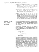
(i) Save the workbook.
Exercise
6:
Using
a
The ability to set constraints is essential
in
optimization problems
but less
so
with the types of problems we are solving. However, for
demonstration purposes, we shall
look

at a simple example of their
use when solving a cubic equation. Suppose we have to find a root
for the equation:
I
.3x3
-
2.45~’
-
0.8~
+
1.25
=
0.
Let
us
further
suppose that the problem that gave rise to this equation tells us that
the value of
x
which interests
us
lies between
1
and
2.
Constraint
(a) Open CHAPIO.XLS and on Sheet6 set up a worksheet to
look
similar to that
in

Figure
IO.
12.
Name the cells
B4:B7.
The only
formula is
in
E4;
it is
=p*D4”3+q*D4“2+r-*D4+s.
Note that we
use ‘r-’ not ‘r’ for the
cell
C6 since Microsoft Excel reserves
the names
‘r’
and ‘c’ for its own use. The value of
1.5
in
D4
is
our initial guess at the root.
I
I
A
I
B
IC1
D

I
E
111
Finding
a
positive
root
of
a
cubic equation
~~
[31 Coefficients
1
I
Roots
I
Function
61
r
I
-0.8
71
S
I
1.25
Figure
10.12
(b) Call up Solver as before. Set the Target Cell to
E4
and specify

zero for required value.
We will now add two constraints. We will specify that
D4
is to be
greater than
I
and less than
2.
(c) Click on the
Add
button
in
the Subject to
the
Constraints area
to bring up the Add Constraint dialog box shown
in
Figure
IO.
13.
In
the Cell Reference box type
D4.
Change the operator
to
‘>=’,
and type
‘
1
’

in
the Constraint box.
Solving
Equations
201
Figure 10.13
Click on the
Add
button
of
the Add Constraint dialog to add
the second constraint. Make this read
D4
<=
2.
Then click on
the
OK
button since we have no more constraints to add.
Figure
10.14
shows the Solver dialog with
two
constraints.
Figure
10.14
(d) Click the
Solve
button. Solver finds an acceptable result. My
values are

D4
=
1.94703739312482

and
E4
=
7.87E-07.
(e) Change the constraint to find the other
two
values. One
of
them is negative
so
the constraint
D4
<=
0 will be appropriate.
The other lies between 0 and
1.
With a starting value
of
0 it
may find a solution with no constraints. Good hunting!
(f)
Save the workbook.
Solver
Options
We shall have little need in these Exercises to alter Solver’s
operational values but the reader may be interested in looking at

them. Click on the Solver dialog
Options
button to open the
Options dialog shown
in
Figure
10.15.
Note:. Avoid having
IF
or
CHOOSE
functions between the
decision variables (the ones
in
By
Changing) and the objective (the
Target Cell) since this will
generally cause Solver
to
fail to
find
a solution.
202
A Guide to Microsoft Excel
2002
for Scientists and Engineers
Use Automatic Scaling
is too technical to explain here.
Figure
10.15

Max
Time
sets the maximum amount of time Solver may spend on
the problem. The default value of
100 seconds
is
ample with a
modern
PC for all but very large problems.
Iterations
sets the limit of the number of attempts Solver has to
find a satisfactory solution.
Precision
pertains to the constraints. Let the Precision be
1
x
and suppose we specify the constraint A1
>=
0.
After some
iterations Solver find a solution but A1
=
-1
x
lo-’
. Solver will
consider the constraint has been met since it is within the precision.
Tolerance
pertains to integer constraints. An integer constraint
makes the problem much harder. Try initially solving without

integer constraints.
Convergence
sets the amount of relative change to allow in the last
five iterations before Solver stops with a solution.
Assume Linear Model
determines which algorithm is used by
Solver. Linear problems are more readily solved.
Solving Equations
203
Assume Non-Negative
ensures that all decision variables (the ones
in By Changing) that are not explicitly given a constraint have a
lower bound of zero.
Explanations of the other options are beyond the scope of this
book. However, as we will see
in
later Exercises, setting
Derivatives to Central can be advantageous when solving for roots
of equations.
Concepts
B:
Solving
A system of linear equations is a set of
n
linear equations
in
which
each equation contains up to
n
variables or ‘unknowns’.

A
simple
example might be to find
x
and
y
given:
Simultaneous
Equations
2x
+
3~
-
3
=
0
3x
+
2~
-
5
=
0
(10.1)
An example that appears more complex might be to find the three
T
values such that
T,
=mg
T2

COS
a
-
T3
COS
p
=
0
T2
sin
a
-
T3
sin
p
-
T,
=
0
(1
0.2)
where
a
=
60°,
p
=
30°,
m
=

10
and
g
=
9.81.
Of course, we would solve these problems using the techniques we
learnt
in
school. Setting up a worksheet to solve a set of
simultaneous equations with only
two or three unknowns would be
an inefficient use of time. It would be worth setting up a worksheet
if we had a large number of similar sets of equations to solve.
Furthermore, the techniques learnt with only three unknowns can
be expanded
to
cases of more variables.
So
let us look at how we
might use Solver to find the values of
x
and
y
in
the first example.
The use
of
matrix algebra to solve
systems
of

equation
is
shown
in
later exercises.
Our use of Solver
so
far has involved single equations. We have
had one
Set Cell
and one
Changing Cell.
The latter was changed to
give the former a near-zero value. Can we apply this method
to
the
two
equations and ask Solver to vary both
x
and
y?
The answer is
a partial yes. We can have more than one
Changing Cell
but there
can be only one
Set Target Cell.
If we have a third cell that sums
the values of the
two

functions, we could get Solver to use this for
Summing the absolute values
its
Set Cell.
That should seem to work; if each function evaluates
would
also
work
but there are
to zero then their sum should be zero. However, there is a problem.
m~thmatical argumentsthat make
What if one cell evaluates to
-4
and the other to
+4?
These will
it better
to
sum squares.
sum to zero but we will not get the correct values for the variables.
Rather than sum the values of the two functions, we will sum the
squares of the values to avoid this ‘cancellation’ problem.
204
A
Guide to Microsoft Excel
2002
for Scientists and Engineers
A
B
C

I
D
-
1
System
of
Linear Equations
2
Exercise
7:
A Simple
We now create a worksheet to solve the simultaneous equations in
Equation 10.1.
Simultaneous
3
4
5
6
Equations Problem
(a) Open CHAP1O.XLS and on Sheet7 set up a worksheet similar
to that in Figure 10.16. The cells with formulas are:
C4:
C5:
D4: =C4"2
D5: =C5"2
D6: =D4+D5
=2*B4
+
3*B5
-

3
=3*B4 + 2*B5
-
5
first equation in Equation
10.1
second equation in Equation 10.1
Variables Equations Squares
X
0 -3
9
SUM
=
34
Y
0 -5
25
(b) Make D6 the active cell and start Solver. The
Set Target Cell
should contain D6. Set
Equal to Value
0
and in the
By
Changing Cells
box, either type B4:B5 or use the mouse to
select them. Alternatively, press the Guess button, and Solver
will correctly set the output cells
to
$B$4:$B$5.

(c) Press Solver's
Solve
button. Solver reports it has found a
solution with 6.8
x
1-13 as the value in D6. This is reasonably
close to zero. The reported values for
x
and
y
are 1.79999988
and
-0.200000
1 1,
respectively. If you replace these with 1.8
and
-0.2,
the equations each evaluate to zero.
So
Solver
is
useful but not perfect.
Solver has improved
with
each new
version
of
Excel.
To solve
this

problem
in
Excel
95
one
had
to
run
Solver twice!
If you open the Solver Options box and select Central
Derivative, Solver gets a result that is even closer to the exact
solutions when
run
with the initial zero values for the
variables.
Exercise
8:
An
Simultaneous
have the general form:
With Exercise 7 behind us we can tackle a more complex problem.
Our task is to construct a worksheet that will help us solve any
system of linear equations with three unknowns. Let the system
Improved
Equations Solver
Solving Equations
205
~
3 Variables Coefficients Formulas
4

x
1 a1 2 bl
4
c-I
5
dl -33 -22
5
y
1
a2
6
b2
6
c-2 7 d2 -70
-51
-
6
z
1 a3
3
b3
-6
c3
4
d3 71 72
7
I
Sum
of
Squares

8269
a,x
+
b,y
+
c,z
-
d,
=
0
a2x+b2y+c2z-d2=0
a3x
+
b3y
+
c3z-d3
=
0
We
shall use three named cells for the variables
x,
y
and
z,
and
12
named cells for the coefficients. Our worksheet will show cells
with text such as ‘a1
’,
‘a2’, etc., but the names will, of course, be

‘al-’, ‘a2-’, etc. We cannot use ‘cl’, etc., as names
so
we will use
‘c-l’, etc., both as text and as names of cells.
As
a
concrete example upon which to design the worksheet, we
will solve the system
of
equations
in
Equation
10.3.
h+
4~+5~-33=0
6x+ 6~+7~-70=0
3~-
6y+4~+71
=O
(1
0.3)
(a) On Sheet8 of
CHAP1
0.XLS
construct a worksheet
as
shown
in
Figure
10.1

7
temporarily ignoring
K4:K7.
The values
of
1
for the variables are arbitrary starting values.
(b) We now need to use InsertlNamelCreate five times; once for
A4:B6,
then with
C4:D6,
etc.
K
Simultaneous Equations Solver
Figure
10.17
(c) Enter the formulas for the three equations
in
the set:
K4:
=al-*x
+
bl-*y
+
c-l*z
+
dl-
K5:
=a2-*x
+

b2-*y
+
c_2*z
+
d2-
K6:
=a3-*x
+
b3-*y
+
c_3*z
+
d3-
(d)
As
before, we need a single cell as the target for Solver. Rather
than computing the sum of the absolute values of the three
functions, we
will
sum their squares with
a
single formula. In
K7
type the formula
SUMSQ(K4:K6)
to achieve this.
(e) We are ready to use Solver. The
Target
cell should be
K7

-the
cell that sums the squares
of
the functions. Make sure to use
Equal
to
Value
of
0,
and set the
By
Changing
Cells
to
B4:B6.
206
A
Guide to Microsoft Excel
2002
for Scientists and Engineers
Changing the option to use Central
Derivatives does involve more
Central. Return to the main Solver dialog by clicking OK.
computational steps but it improves
the accuracy
of
the result with
problems such as these.
Open the Option dialog, locate the Derivative area and select
(f)

Now click the Solve button. The results are
x
=
6.0,
y
=
1
1.5
the
and
z
=
-5.0.
The first equation evaluates to -1.6
x
other
two
to zero.
(g) Save the workbook.
Exercise
9:
Non-
The simultaneous equations we have solved so far were all linear.
These could have been solved using simple algebraic techniques.
Non-linear systems
of
equations are far more difficult to solve with
paper and pencil, requiring a knowledge of calculus. Let's see if
linear Simultaneous
Equations Solver

Solver is capable of coming to our aid. We will solve the non-
linear simultaneous equations:
x2
+
2y2- 22.0
=
0
-2x*+xy
-3y+ 11.0=0
(a) Figure 10.18 shows the required worksheet with the cell
contents displayed as formulas. Set this up on Sheet9
of
CHAPl0.XLS. Note that cells in B3:B4 have the names shown
to their left. The required formulas are:
D3:
D4:
=~"2
+
2*y"2
-
22
=-2*~"2
+
X*Y
-
3*y
+
11
D5: =SUMSQ(D3:D4)
I

A
B
C
D
1
ISvstern
of
Non-linear Eauations
Figure 10.18
(b) Call up Solver. We need to make D5 the target cell and B3:B4
the cells to be varied to equate the target cell to
0.
Again it will
be useful, but not essential, to use central derivatives.
With starting values of
1
for both variables Solver suggests an
approximate solution with
x
=
1.99994 and
y
=
3.00004.
The function evaluate to values somewhat larger than
0.
Experimentation shows
x
=
2

and
y
=
4 is an exact solution. Of
course, since the equations contain
2
and?, multiple solutions are
Solving Equations
207
possible. Starting with
0
for each variable, Solver reported
x
=
-0.2763 and
y
=
3.3 109 as a solution.
(c) Save the workbook.
Concepts C: Matrix
The Microsoft Excel matrix functions are:
MDETERM(A)
Returns the matrix determinant of an array.
Algebra
MINVERSE(A) Returns the inverse of the matrix of an array.
MMULT(A,B) Returns the matrix product.
TRANSPOSE(A) Returns the transpose of an array. The first
row of the input array becomes the first
column of the output array, etc.
Some points to watch for when using matrix functions:

(i)
For all but TRANSPOSE(), every cell in the array must
contain
a numeric value otherwise the #VALUE! error
results.
(ii)
The #VALUE! error results when an illegal matrix operation
is attempted.
(iii) Because the first
two
functions use an accuracy
of
16
digits,
small numeric errors may occur. For example, a singular
array may return a result that differs from zero by 1E-16.
(iv)
Except for MDTERMO, these are array functions and must
be completed with
(Ctrll+[Shift]+[Entercl].
Before we use these functions, a brief review of matrix algebra
may help.
1.
A matrix with
m
rows and
n
columns is said to be of order
m
x

n.
When
n
and
m
are equal, the matrix is said to be square.
2.
Matrix
A
is said to be identical to matrix
B
when every element
inA equals the corresponding element
in
B,
i.e.
a,,
=
b,
.Clearly
the
two
matrices must have the same order.
If
when
using
a
matrix
You
get

one
value rather than many,
then you have forgotten either
(i)
to
select a range before entering the
formula
or
(ii) to complete the
entry using
[Ctrlj+[mShlft+/W].
208
A
Guide
to
Microsoft Excel
2002
for
Scientists and Engineers
3.
IfA
and
B
are
of
the same order, then
A
+
B
=

C,
and
C
has the
same order as
A
and
B.
The elements
in
C
are found using
c,,
=
a,,
+
b,,.
Matrix subtraction
is
defined
in
a manner
similar
to addition.
4.
If
A
is
a
matrix of order

m
x
n
and B
is
a matrix
of
order
n
x
p
(Le. the number
of
columns
in
A
equals the number
of
rows
in
B),
then the
matrixproduct
ofA
and
B, AB,
is defined and is a
matrix
of
order

m
x
p.
IfAB
=
C,
then
n
5.
Matrix multiplication
is
not commutative; AB does not
necessarily equal
BA.
6. Matrix division
is
undefined.
7.
An
identity matrix,
I,
is
a square matrix in which the elements
on the main diagonal have values
of
1
and all others have
values
of zero.
8.

Let
A
be a square matrix. Then the
inverse
ofA, represented by
A-',
is
defined as the matrix which when multiplied by
A
yields
an identity matrix. Thus, we see
A-'
=
I.
If
B
is the inverse of
A,
then
A
is
the inverse
of
B
and
BA
=
I
=AB.
9.

A
matrix which has no inverse is said to be
singular.
10.
When a matrix
A
is
multiplied by an identity matrix, the result
is
A; IA =A.
Exercise
1
0:
Some
In
this exercise we demonstrate some ofthe topics reviewed above.
We will find the sum of
two
matrices, find a matrix inverse, and
Matrix
Operations
show
that
RA-l
=
I.
(a) Open the workbook
CHAP1
0.XLS
and move to Sheet

10.
Enter
the text and values shown
in
AI
:G3
of
Figure
10.19.
Use
the
Merge
and Center
tool to centre the text over
two
columns.
(b) Enter the values in A4:E5.
(c)
We now find the elements of
C
such that
A
+
B
=
C.
In
G4
enter the formula =A4+D4. Copy this to
G4:H5.

Solving
Equations
209
Figure
10.19
(d) Enter the text row
7
and centre each across
two
columns.
To
get superscripts, select the text (such as
-1)
and use the
command FgmatlCells and put
a
check
mark
in
the
Superscript
box on the Font dialog box.
(e) Enter the values
in
A8:B9. These are the elements
of
matrix
D.
(f)
To compute the inverse

of
D,
select the range D8:E9. Enter the
formula=MINVERSE(A9:B9) and press[+)+(~Shift+I~].
(8)
To
show that
DD-'
=
I,
select
G8:H9.
Enter the formula
=MMULT(A8:B9, D8:ES) and press~+[~Shift+[~]]. You
may wish
to
use the Formula Palette: type =MMULT, press
m+A.
Do
not click the
OK
button on the Formula Palette,
use
ICtrl)+(73iKShift+[W].
Note that the main diagonal elements have values
of
1.
We
expected the off-diagonal elements to have values
of

zero but
in
HS
we have -2.8E-17. Recalling restriction (iv) above (Microsoft
Excel uses a precision
1
E-16
in
computing matrix functions) we
shall accept this value as zero.
If
you replace the values
in
the first
row by
-1
and
2,
and
in
the second row by
2
and
5,
the
off-
diagonal elements compute to identically zero.
(h)
The formula =MDETERM(A8:BS)
in

A12
computes the
determinant
of
the square matrix
D.
No
inverse matrix exists
for a matrix with a zero determinant. The formula
in
B
12
is
=I
F(A12=O,"Singular","Non-singular").
(i) Save the workbook.
21 0
A
Guide to Microsoft Excel
2002
for Scientists and Engineers
Exercise
11
:
Solving
Equations
3x+4y=
17
A
system of linear equations may be represented

in
matrix form.
Thus the system of
two
equations:
x-2y
=-1
Systems
of
Linear
may be represented by:
Equation
M
Performing the matrix multiplication in Equation
M,
we get:
["'"I=
3x
+
4y
[;;I
When matrix
A
and matrixB are equal, the corresponding elements
are equal.
So
it follows that
x
+
2y

=
14
and
2x
-y
=
5;
these are
the equations with which we started, thereby justifying the
statement that we may represent a system of linear equations
in
matrix form.
In
the following
A
represents the matrix
of
the coefficients,
X
the
matrix of the variables and
C
the matrix of the constants.
Let
us
write Equation M in the form:
Ax
=c
Multiply both sides by the inverse of
A

giving
L'Ax
=
A-'C
But sincek'A
=
I,
this becomes
IX
=
A-'C
We know that
IX
=
X,
therefore
x
=
A-'C
From this we see that the value ofthexmatrix may be obtained by
computing
A-'C.
In
Exercise
10
we found the inverse of this
matrix,
so
we may write:
[;I=[

-0.3
Oa4
O-'][-']
0.1
17
Performing the multiplication gives
L:l=l:l
From which we see that
x
=
3
and
y
=
2.
Solving Equations
21
I
This may have left you less than impressed; you could have solved
the
two
simultaneous equations in your head. But the method may
be applied to more challengingproblems. In this exercise we solve:
2x
+
3~
-
22
=
15

3x
-
2y
+
22 =-2
4x-
y+
32
=
2
The completed worksheet will resemble that in Figure
10.20.
(a) Open workbook
CHAP 1O.XLS
and move to Sheet
1
1.
Enter the
text in rows
1,2,3,9
and
14.
(b)
In
A5:C7
enter the coefficients ofthe equations, and in
D5:D7
If
typing
(C)

results
in
the
enter the constants.
copyright symbol
0,
use
-
ToolslAutoCorrect
to
remove
this
(c) The next step is to compute the inverse
(k')
of the matrix of
from
the list
of
automatic
coefficients. Select the range A
1O:C 12,
enter the formula
corrections.
=MINVERSE(A5:C7)
and press
[CtrlJ+[oShift+[%3].
The
cells shown in the figure were formatted to display five places.
(d) The final step to find the solutions is to compute
A-'C.

Select
D10:D12,
enter the formula
=MMULT(AlO:C12, D5:D7)
and
press
[Ctrlj+[ShiftJ+[].
The solutions have now been found. We may wish to check that
these agree with the system of equations.
(e) Use InsertlN_ame to name the cells
D5:D7
as
x,
y
and
z,
respectively.
(f)
The formulas in row 15 are:
A15:
=A5*x
B15:
=B5*y
C15:
=C5*z
D15:
=SUM(A15:C15)
Use AutoSum to make this.
These formulas are copied down to row
17.

The values in
D15:D17
agree with those in
D5:D7,
thus confirming that we
have solved the system of equations.