Functional MRI data analysis detection, estimation and modelling
Bạn đang xem bản rút gọn của tài liệu. Xem và tải ngay bản đầy đủ của tài liệu tại đây (2.66 MB, 206 trang )
FUNCTIONAL MRI DATA ANALYSIS: DETECTION,
ESTIMATION AND MODELLING
LUO HUAIEN
(M.Eng., Huazhong University of Science and Technology)
A THESIS SUBMITTED
FOR THE DEGREE OF DOCTOR OF PHILOSOPHY
DEPARTMENT OF ELECTRICAL & COMPUTER
ENGINEERING
NATIONAL UNIVERSITY OF SINGAPORE
2007
Acknowledgements
I would like to thank all those who provided invaluable advice and assistance to my
research work during the past four years in the National University of Singapore.
First of all, I would like to express my deepest gratitude to my advisor Dr. Sada-
sivan Puthusserypady for his patient discussion, inspiring encouragement and prompt
guidance.
My special thanks also go to my dear parents. It is their love that lead me through
many difficulties.
I also would like to thank my friend Zheng Yue, who plays a pivotal role during the
course of my Ph.D studies and especially helps me to recover from many setbacks.
Thanks to my friends Chen Huiting, Zhou Xiaofei, Zuo Ziqiang, Zhang Jing, Rajesh,
Ajeesh, Wang Zhibing etc for all the good times we had together.
Luo Huaien
June 2007
i
Contents
Acknowledgements i
Summary vii
List of Tables x
List of Figures xii
List of Abbreviations xvii
List of Symbols xx
1 Introduction 1
1.1 Functional Magnetic Resonance Imaging . . . . . . . . . . . . . . . . 4
1.1.1 Nuclear Magnetic Resonance – the Basis . . . . . . . . . . . . 6
1.1.2 Magnetic Resonance Imaging . . . . . . . . . . . . . . . . . . 10
1.1.3 BOLD Functional MRI . . . . . . . . . . . . . . . . . . . . . . 13
1.1.4 Hemodynamic Response . . . . . . . . . . . . . . . . . . . . . 15
ii
Contents iii
1.1.5 Experimental Designs in fMRI . . . . . . . . . . . . . . . . . . 17
1.1.6 Description of the Experimental Data Used in This Thesis . . . 20
1.2 fMRI Data Analysis . . . . . . . . . . . . . . . . . . . . . . . . . . . . 21
1.2.1 Preprocessing . . . . . . . . . . . . . . . . . . . . . . . . . . . 21
1.2.2 Modelling the fMRI Data . . . . . . . . . . . . . . . . . . . . . 22
1.2.3 Data Analysis and Inference . . . . . . . . . . . . . . . . . . . 28
1.3 Thesis Contribution and Organization . . . . . . . . . . . . . . . . . . 34
2 Sparse Bayesian Method for Determination of Flexible Design Matrix in
fMRI Data Analysis 37
2.1 Introduction . . . . . . . . . . . . . . . . . . . . . . . . . . . . . . . . 37
2.2 General Linear Model . . . . . . . . . . . . . . . . . . . . . . . . . . . 39
2.3 Sparse Bayesian Learning . . . . . . . . . . . . . . . . . . . . . . . . . 41
2.4 Results and Discussion . . . . . . . . . . . . . . . . . . . . . . . . . . 44
2.4.1 Simulated Data . . . . . . . . . . . . . . . . . . . . . . . . . . 45
2.4.2 Experimental fMRI Data . . . . . . . . . . . . . . . . . . . . . 50
2.5 Conclusion . . . . . . . . . . . . . . . . . . . . . . . . . . . . . . . . 52
3 fMRI Data Analysis with Nonstationary Noise Models: A Bayesian Ap-
proach 54
3.1 Introduction . . . . . . . . . . . . . . . . . . . . . . . . . . . . . . . . 54
3.2 Nonstationary Noise Models . . . . . . . . . . . . . . . . . . . . . . . 56
3.2.1 Time-varying Variance Model . . . . . . . . . . . . . . . . . . 56
3.2.2 Fractional Noise Model . . . . . . . . . . . . . . . . . . . . . . 59
3.3 Bayesian Estimator . . . . . . . . . . . . . . . . . . . . . . . . . . . . 62
3.4 Results and Discussion . . . . . . . . . . . . . . . . . . . . . . . . . . 66
3.4.1 Simulated Data . . . . . . . . . . . . . . . . . . . . . . . . . . 66
Contents iv
3.4.2 Experimental fMRI Data . . . . . . . . . . . . . . . . . . . . . 73
3.5 Conclusion . . . . . . . . . . . . . . . . . . . . . . . . . . . . . . . . 75
4 Analysis of fMRI Data with Drift: Modified General Linear Model and
Bayesian Estimator 78
4.1 Introduction . . . . . . . . . . . . . . . . . . . . . . . . . . . . . . . . 78
4.2 Models . . . . . . . . . . . . . . . . . . . . . . . . . . . . . . . . . . 80
4.2.1 Noise Model . . . . . . . . . . . . . . . . . . . . . . . . . . . 81
4.2.2 Drift Model . . . . . . . . . . . . . . . . . . . . . . . . . . . . 81
4.3 Modified GLM . . . . . . . . . . . . . . . . . . . . . . . . . . . . . . 82
4.4 Model Selection . . . . . . . . . . . . . . . . . . . . . . . . . . . . . . 84
4.5 Results and Discussion . . . . . . . . . . . . . . . . . . . . . . . . . . 85
4.5.1 Simulated Data . . . . . . . . . . . . . . . . . . . . . . . . . . 85
4.5.2 Experimental fMRI Data . . . . . . . . . . . . . . . . . . . . . 89
4.6 Conclusion . . . . . . . . . . . . . . . . . . . . . . . . . . . . . . . . 91
5 Adaptive Spatiotemporal Modelling and Estimation of the Event-related
fMRI Responses 92
5.1 Introduction . . . . . . . . . . . . . . . . . . . . . . . . . . . . . . . . 92
5.2 HDR Function . . . . . . . . . . . . . . . . . . . . . . . . . . . . . . . 94
5.3 Spatial and Temporal Adaptive Estimation . . . . . . . . . . . . . . . . 96
5.3.1 Model derivation . . . . . . . . . . . . . . . . . . . . . . . . . 96
5.3.2 Extension to Multiple Events . . . . . . . . . . . . . . . . . . . 99
5.3.3 Relation to the Canonical Correlation Analysis . . . . . . . . . 100
5.4 Results and Discussion . . . . . . . . . . . . . . . . . . . . . . . . . . 103
5.4.1 Simulated data . . . . . . . . . . . . . . . . . . . . . . . . . . 103
5.4.2 Experimental fMRI Data . . . . . . . . . . . . . . . . . . . . . 113
Contents v
5.5 Conclusion . . . . . . . . . . . . . . . . . . . . . . . . . . . . . . . . 114
6 Estimation of the Hemodynamic Response of fMRI Data using RBF Neural
Network 117
6.1 Introduction . . . . . . . . . . . . . . . . . . . . . . . . . . . . . . . . 117
6.2 Volterra Series Model . . . . . . . . . . . . . . . . . . . . . . . . . . . 119
6.3 Neural Networks Model . . . . . . . . . . . . . . . . . . . . . . . . . 122
6.3.1 Relation between RBF neural network and Volterra series . . . 124
6.3.2 Learning procedure . . . . . . . . . . . . . . . . . . . . . . . . 127
6.4 Balloon Model . . . . . . . . . . . . . . . . . . . . . . . . . . . . . . 128
6.5 Results and Discussion . . . . . . . . . . . . . . . . . . . . . . . . . . 130
6.5.1 Simulated Data . . . . . . . . . . . . . . . . . . . . . . . . . . 130
6.5.2 Experimental Data . . . . . . . . . . . . . . . . . . . . . . . . 141
6.6 Conclusion . . . . . . . . . . . . . . . . . . . . . . . . . . . . . . . . 144
7 NARX Neural Networks for Dynamical Modelling of fMRI Data 146
7.1 Introduction . . . . . . . . . . . . . . . . . . . . . . . . . . . . . . . . 146
7.2 NARX Model . . . . . . . . . . . . . . . . . . . . . . . . . . . . . . . 147
7.3 Results and Discussion . . . . . . . . . . . . . . . . . . . . . . . . . . 148
7.3.1 Simulated Data . . . . . . . . . . . . . . . . . . . . . . . . . . 148
7.3.2 Experimental fMRI Data . . . . . . . . . . . . . . . . . . . . . 152
7.4 Conclusion . . . . . . . . . . . . . . . . . . . . . . . . . . . . . . . . 154
8 Conclusion and Future Directions 157
8.1 Summary and Conclusions . . . . . . . . . . . . . . . . . . . . . . . . 157
8.2 Future Directions . . . . . . . . . . . . . . . . . . . . . . . . . . . . . 159
Bibliography 162
Contents vi
A Derivation of Eq. (3.22) and Eq. (3.23) 175
B Derivation of Eq. (3.27) to Eq. (3.29) 177
B.1 Compute the the objective function L . . . . . . . . . . . . . . . . . . 177
B.2 Derivatives and updates . . . . . . . . . . . . . . . . . . . . . . . . . . 178
B.3 A special case . . . . . . . . . . . . . . . . . . . . . . . . . . . . . . . 179
C Derivation of Eq. (4.14) 181
D Papers Originated from this Work 183
Summary
Functional Magnetic Resonance Imaging (fMRI) is an important technique for neu-
roimaging. Through the analysis of the variation of blood oxygenation level-dependent
(BOLD) signals, fMRI links the function of the brain and its underlying physical struc-
tures by using the MRI techniques. The low signal-to-noise ratio (SNR) and complexity
of the experiment poses major difficulties and challenges to the analysis of fMRI data.
This thesis presents robust (less false positive rate) and efficient (easy estimation
procedure) signal processing methods for fMRI data analysis. It aims to complement
the current methods of fMRI data analysis in order to achieve accurate detection of the
activated regions of the brain, better estimation of the hemodynamic response (HDR) of
the brain functions and modelling of the dynamics of fMRI signal.
The fMRI data are first investigated under the Bayesian framework. Based on the
conventional general linearmodel (GLM), a flexible designmatrix determination method
through sparse Bayesian learning is proposed. It integrates the advantages of both data-
driven and model-driven analysis methods. This method is then extended to incorporate
the nonstationary noise to the model. Two nonstationary noise (time-varying variance
vii
Summary viii
noise and fractional noise) models are examined. The covariance matrices of these two
noises share common properties and are successfully estimated using a Bayesian esti-
mator. Considering that the fMRI signal also contains drift, a modified GLM model
is proposed which could effectively model and remove the drift in the fMRI signal.
Through mathematical manipulations, updating algorithms are derived for these pro-
posed methods. The proposed Bayesian estimator could provide accurate probability
of the activation and hence avoid the multiple comparison problems encountered in the
traditional null hypothesis methods.
The second part of the thesis is focused on the estimation of the HDR of the human
brain. Both linear and nonlinear properties of the event-related fMRI experiment are
examined based on the inter-stimulus intervals (ISI). A linear spatiotemporal adaptive
filter method is proposed to model the spatial activation patterns as well as the HDR.
The equivalence of the proposed method to the canonical correlation analysis (CCA)
method is also demonstrated. It is reported that when the ISI is small, the fMRI signal
shows nonlinear properties. Thus, nonlinear methods of fMRI signal analysis are also
examined. A method based on the radial basis function (RBF) neural network is pro-
posed to regress the measured fMRI signal on the input stimulus functions. The relation
between the parameters of the RBF neural network and Volterra series are demonstrated.
The HDR is then obtained from the parameters of the RBF neural network which shows
significant advantages.
The third part of the thesis examines the nonlinear autoregressive with exogenous
inputs (NARX) neural network to model the fMRI signal. With the knowledge of exper-
imental paradigm (input) and measured data (output), the NARX neural network could
identify the complex human brain system and reconstruct the BOLD signal from noisy
fMRI signal. This results in an enhanced SNR of the measured signal and a robust
estimation of the activated regions of the brain.
Summary ix
Extensive simulation studies on synthetic as well as experimental fMRI data are car-
ried out in this thesis. Results show that these methods could complement the traditional
methods to cope with the difficulties and challenges in fMRI data analysis. This may
contribute to the better understanding of the nature of the fMRI signal as well as the
underlying mechanisms.
List of Tables
1.1 Major techniques used for the study of brain functioning . . . . . . . . 3
1.2 Comparison of different TR, TE and pulse sequence used in different
MR contrast images. . . . . . . . . . . . . . . . . . . . . . . . . . . . 9
2.1 The error rate of different
t
-value thresholds for different types of signals 49
3.1 Standard deviation (SD) of estimated ˆw on simulated data with different
weight and noise. . . . . . . . . . . . . . . . . . . . . . . . . . . . . . 67
3.2 Standard deviation (SD) of estimated ˆw on simulated data with different
weight and Hurst exponent. . . . . . . . . . . . . . . . . . . . . . . . . 72
4.1 Comparison of estimated variance of wavelet coefficients of noise at
different scale with the true value. . . . . . . . . . . . . . . . . . . . . 87
4.2 Model selection of CIC, AIC
c
and SIC criteria. . . . . . . . . . . . . . 87
4.3 MSE comparison of three model selection criteria with drift added. . . . 88
4.4 MSE comparison of three model selection criteria without drift. . . . . 89
5.1 Relation of the levels of the noise variances and the coefficients of the
spatial adaptive filter for a 3 × 3 window. . . . . . . . . . . . . . . . . 106
x
List of Tables xi
5.2 Comparison of the proposed adaptive filter method, CCA and GLM for
the estimation of HDR. . . . . . . . . . . . . . . . . . . . . . . . . . . 108
6.1 Estimation of Volterra kernel parameters (P = 2) . . . . . . . . . . . . 133
6.2 Estimation of Volterra kernel parameters usingRBF neural network method
and least-squares (LS) method when the highest order of Volterra series
is 3. . . . . . . . . . . . . . . . . . . . . . . . . . . . . . . . . . . . . 135
List of Figures
1.1 Some milestones in the development of fMRI. . . . . . . . . . . . . . . 5
1.2 Illustration of the spins’ alignment at equilibrium before (left side) and
after (right side) the magnitude field B
0
is applied. . . . . . . . . . . . 7
1.3 Three types of MR images of the same slice in the brain. . . . . . . . . 10
1.4 Three stages in the formation of MR images. . . . . . . . . . . . . . . . 12
1.5 Illustration of the slice selection. . . . . . . . . . . . . . . . . . . . . . 12
1.6 Illustration of the change of deoxyhemoglobin content in the venous
blood when the neuron is in the baseline (left) and active (right) states.
In active state, the oversupply of oxygen by CBF results in the decrease
of the concentration of deoxyhemoglobin. . . . . . . . . . . . . . . . . 14
1.7 Physiological changes accompanying brain activation . . . . . . . . . . 16
1.8 Schematic representations of the fMRI BOLD hemodynamic responses.
(a) HDR to a single short duration event; (b) HDR to a block of multiple
consecutive events. . . . . . . . . . . . . . . . . . . . . . . . . . . . . 17
1.9 The basic steps in an fMRI experiment. . . . . . . . . . . . . . . . . . 18
xii
List of Figures xiii
1.10 Illustration of BOLD signals of (a) block design and (b) event-related
design. . . . . . . . . . . . . . . . . . . . . . . . . . . . . . . . . . . . 19
1.11 fMRI data acquisition as a system with input and output. . . . . . . . . 23
2.1 Illustration of a block design and its square waveform representation. . . 45
2.2 A simulated BOLD signal corrupted by drift and noise (Type 3) is de-
composed by the proposed approach into different sources. (a) Simu-
lated noisy fMRI signal; (b) BOLD response; (c) Constant mean value;
(d) Slowly varying drift; (e) Noise. . . . . . . . . . . . . . . . . . . . 46
2.3 The simulated signals and their reconstruction. (a) Type 1: BOLD re-
sponse corrupted by noise; (b) Type 2: No BOLD response, only noise;
(c) Type 4: No BOLD response, only noise and drift. . . . . . . . . . . 48
2.4 ROC curves for simulated noisy data (2D plus time). . . . . . . . . . . 51
2.5 Results of fMRI data analysis to a visuospatial processing task. (a) Con-
ventional
t
-test (
t
> 3.8, p < 0.05); (b) The proposed method with
Sparse Bayesian Learning (
t
> 6.3, p < 0.05). . . . . . . . . . . . . . . 52
3.1 Detection results of simulated fMRI data using different methods: (a)
OLS method with thresholded statistical parametric map (SPM) (t >
1.7, p < 0.05); (b) WLS method with thresholded SPM (t > 1.7, p <
0.05); (c) Bayesian method with posterior probability map (PPM) (P (effect >
0.4) > 0.9). . . . . . . . . . . . . . . . . . . . . . . . . . . . . . . . . 69
3.2 ROC curves for simulated noisy data: (a) for i.i.d. noise; (b) for time-
varying variance noise. . . . . . . . . . . . . . . . . . . . . . . . . . . 70
3.3 Detection results of simulated data using fBm noise model: (a) OLS
in time domain with thresholded SPM (t > 3.4, p < 0.001); (b) OLS
in wavelet domain with thresholded SPM (t > 3.4, p < 0.001); (c)
Bayesian method in wavelet domain with PPM (P(effect > 1) > 0.99). 74
3.4 ROC curves of OLS (in both time domain and wavelet domain) and
Bayesian (after DWT) methods for simulated fMRI data corrupted with
fBm noises. . . . . . . . . . . . . . . . . . . . . . . . . . . . . . . . . 74
List of Figures xiv
3.5 Results of a block visuospatial processing task fMRI data: (a) thresh-
olded SPM of OLS method (t > 3.4, p < 0.001, uncorrected); (b)
thresholded SPM of WLS method (t > 3.4, p < 0.001, uncorrected); (c)
thresholded SPM of OLS method with Bonferroni correction (t > 7, p <
0.05, corrected); (d) thresholded SPM of WLS method with Bonferroni
correction (t > 7, p < 0.05, corrected); (e) PPM of Bayesian method
using time-varying variance noise model (P (effect > 0.8) > 0.99);
(f) PPM of Bayesian method using fractional noise model (P (effect >
0.8) > 0.99). . . . . . . . . . . . . . . . . . . . . . . . . . . . . . . . 76
4.1 Simulated fMRI signal. . . . . . . . . . . . . . . . . . . . . . . . . . . 86
4.2 Simulated fMRI signal and the estimated drift. . . . . . . . . . . . . . . 88
4.3 Results of the proposed method to a visuospatial processing task (t >
5.3 P < 0.05). . . . . . . . . . . . . . . . . . . . . . . . . . . . . . . . 90
4.4 Time series in one voxel and the estimated drift. . . . . . . . . . . . . . 90
5.1 Simulated HDR functions for different parameter settings. (a) different
values of d
1
while keeping c = 0.35 constant; (b) different values of c
while keeping d
1
= 5.4 constant. . . . . . . . . . . . . . . . . . . . . . 95
5.2 Illustration of the spatial smoothing filter and temporal modelling filter. 97
5.3 Spatio-temporal adaptive modelling of the fMRI system . . . . . . . . . 99
5.4 Simulated BOLD signal. (a) pure BOLD signal and the timing of the
stimuli; (b) noisy BOLD signal corrupted with Gaussian white noise. . . 104
5.5 Learning curve of LMS algorithm for spatiotemporal adaptive filter. . . 106
5.6 The HDRs estimated by the spatio-temporal adaptive filter and CCA
methods. . . . . . . . . . . . . . . . . . . . . . . . . . . . . . . . . . . 107
5.7 Estimated HDRs to two event types using the proposed method. . . . . 110
5.8 Detection results of simulated fMRI data: (a) Simulated activation pat-
tern; (b) GLM without spatial smoothing (t > 3); (c) GLM with spatial
smoothing the FWHM is 3 voxel (t > 3); (d) GLM with spatial smooth-
ing the FWHM is 5 voxel (t > 3); (e) Spatio-temporal adaptive filter
method (ρ > 0.3). . . . . . . . . . . . . . . . . . . . . . . . . . . . . . 112
List of Figures xv
5.9 ROC curves for simulated noisy data. . . . . . . . . . . . . . . . . . . 113
5.10 One slice showing the activation of the auditory cortex (ρ > 0.5). . . . . 114
5.11 The estimation of HDRs for the activated voxels using the proposed
adaptive filter method and CCA method. (a) One voxel in the left audi-
tory cortex; (b) One voxel in the right auditory cortex. . . . . . . . . . . 115
6.1 The structure of the RBF neural network. . . . . . . . . . . . . . . . . 123
6.2 Schematic diagram for Balloon model. . . . . . . . . . . . . . . . . . . 130
6.3 One realization of the input signal and the simulated output signal using
Eq. (6.29). (a) Input signal; (b) Output signal. . . . . . . . . . . . . . . 131
6.4 Simulated BOLD signal generated by the Balloon model and noisy BOLD
signals with different additive noise. (a) Simulated pure BOLD signal
and the timing of the stimuli; (b) Simulated noisy BOLD signal cor-
rupted with additive Gaussian white noise; (c) Simulated noisy BOLD
signal corrupted with additive autocorrelation noise. . . . . . . . . . . . 137
6.5 Estimated 1
st
(a) and 2
nd
order (b) Volterra kernels using the proposed
neural network method with SNR = −7dB. . . . . . . . . . . . . . . . 139
6.6 Estimated 1
st
(a) and 2
nd
order (b) Volterra kernels using the proposed
neural network method with SNR = 0dB. . . . . . . . . . . . . . . . . 139
6.7 Estimated 1
st
(a) and 2
nd
order (b) Volterra kernels using the proposed
neural network method when the additive noise is autocorrelational. . . 141
6.8 Estimated 1
st
order Volterra kernels of the left and right auditory cortex
for two subjects. (a) Subject 1; (b) Subject 2. . . . . . . . . . . . . . . 143
6.9 One slice showing the activation of the auditory cortex (R > 0.3). . . . 144
7.1 Schematic diagram for NARX model. . . . . . . . . . . . . . . . . . . 148
7.2 Simulated BOLD signal and its reconstruction from the NARX neural
network. . . . . . . . . . . . . . . . . . . . . . . . . . . . . . . . . . . 150
7.3 The estimated HDR of the simulated data. . . . . . . . . . . . . . . . . 151
7.4 One slice showing the activation of the auditory cortex (R > 0.3). . . . 153
List of Figures xvi
7.5 Comparison between the estimated HDR from the NARX model and the
HDR formulated by difference of two Gamma functions. . . . . . . . . 154
7.6 Time courses of an activated and an inactivated voxel for the real block
experimental fMRI data. . . . . . . . . . . . . . . . . . . . . . . . . . 155
List of Abbreviations
AIC
Akaike Information Criterion
AR
Autoregressive
ARD
Automatic Relevance Determination
ARX
Autoregressive Model with Exogenous Inputs
ATP
Adenosine Triphosphate
BLUE
Best Linear Unbiased Estimator
BOLD
Blood Oxygenation Level Dependent
BSS
Blind Source Separation
CBF
Cerebral Blood Flow
CBV
Cerebral Blood Volume
CCA
Canonical Correlation Analysis
CIC
Confidence Interval Criterion
CMRO
2
Cerebral Metabolic Rate of Oxygen
DCT
Discrete Cosine Transform
DWT
Discrete Wavelet Transform
xvii
List of Abbreviations xviii
EEG
Electroencephalography
EPI
Echo Planar Imaging
ERP
Event-Related Potentials
FIR
Finite Impulse Response
fMRI
Functional Magnetic Resonance Imaging
FPR
False Positive Ratio
FWHM
Full Width at Half Maximum
GLM
General Linear Model
GLS
Generalized Least Squares
GRE
Gradient-Echo Imaging
HDR
Hemodynamic Response
HRF
Hemodynamic Response Function
ICA
Independent Component Analysis
ICA-R
ICA with Reference
ISI
Inter-Stimulus Intervals
KLT
Karhunen-Lo
´
eve Transform
LMS
Least Mean Square
LS
Least Squares
LTI
Linear Time-Invariant
MEG
Magnetoencephalography
MLP
Multi-Layer Perceptrons
MR
Magnetic Resonance
MRI
Magnetic Resonance Imaging
MSE
Mean Square Errors
NARX
Nonlinear Autoregressive with Exogenous Inputs
NMR
Nuclear Magnetic Resonance
List of Abbreviations xix
NMSE
Normalized Mean Square Error
OLS
Ordinary Least Squares
PCA
Principal Component Analysis
PEB
Parametric Empirical Bayesian
PET
Positron Emission Tomography
PPM
Posterior Probability Map
RBF
Radial Basis Function
rCBF
regional CBF
RF
Radio Frequency
ROC
Receiver Operator Characteristic
SD
Standard Deviation
SE
Spin-Echo Imaging
SI
Spiral Imaging
SIC
Schwartz Information Criterion
SNR
Signal-to-Noise Ratio
SOM
Self-Organizing Maps
SPM
Statistical Parametric Mapping
TE
Echo Time
TMS
Transcranial Magnetic Stimulation
TPR
True Positive Ratio
TR
Repetition Time
WLS
Weighted Least Squares
List of Symbols
a
0
Zeroth-order Volterra Kernel
a
1
First-order Volterra Kernel
a
2
Second-order Volterra Kernel
B
0
Static Magnetic Field
B
1
Radio-frequency Pulse
B
Noise Precision Matrix
b
BOLD Response Vector
c
Contrast Vector
d(n) Desired Signal
f Drift
f
Drift Vector
G(t) Magnetic Field Gradient
h(t) Hemodynamic Response Function (HRF)
M
0
Initial Magnetization
M
z
Magnetization along z direction
xx
List of Symbols xxi
M
xy
Magnetization in the xy plane
r
Residual Vector
S
Scaling Matrix
s(n) Stimulus Signal
w
Weight Vector
y
b
(t) BOLD Response
y
Data Vector
Noise
Noise Vector
ρ
Correlation Coefficient
σ
2
Variance
γ
Gyromagnetic Ratio
Ψ
Normal cumulative distribution function
φ Regressors in the Design Matrix
Φ
Design Matrix in GLM
Σ
Noise Covariance Matrix
Λ
Weight Covariance Matrix
Chapter 1
Introduction
If you know, to recognize that you know, if you don’t know, to realize that
you don’t know: That is knowledge. —— Confucius
The brain is the most amazing organ in the human body and the most mysterious
as well as complex. With the development of cognitive neuroscience, many mysteries
are gradually becoming clear to us. Cognitive neuroscience reveals the relation between
cognitive processes (the immaterial mind) and the material brain [1] [2]. It shows what
happens in the brain when human beings are thinking, talking, learning, memorizing,
seeing, acting, etc. To study these cognitive processes in terms of brain-based mech-
anisms (i.e., which parts of the brain are involved, in what kind of ways, what is the
neural basis underlying these processes), many measurement methods have been devel-
oped. These measurement methods can be grouped into four categories: the drug-based
methods, lesion-based methods, electrophysiological methods and neuroimaging meth-
ods. Drug-based methods are used to study how the human brain functions under the
control of drugs. Lesion-based methods analyze the influence of naturally occurring le-
sions or that of “virtual lesions” induced by transcranial magnetic stimulation (TMS) [3]
on the brain’s functioning. Electrophysiological methods measure the action potentials
1
2
or ensemble ofthe brain action potentials during the execution of a specific task [4]. It in-
cludes single-cell recordings, multiple-cells recordings, electroencephalography (EEG),
event-related potentials (ERP) and magnetoencephalography (MEG). Although these
methods show good temporal resolutions, they provide little spatial information about
the activation regions of the human brain. With the help of neuroimaging methods, these
functional images of the physiological processes can be visualized. The neuroimaging
methods include positron emission tomography (PET) and functional magnetic reso-
nance imaging (fMRI) [5]. These four categories of measurement methods in cognitive
neuroscience complement each other to give detailed structural (at which region the neu-
ral activities occur) and functional explanations (in which way the brain functions) of
the cognitive processes. Table 1.1 shows the summary of the properties of these major
methods used in the measurements of the cognitive neuroscience.
As shown in Table 1.1, fMRI possesses advantages of non-invasiveness as well as
better spatial and temporal resolution (It has better spatial resolution compared to EEG
and MEG andbetter temporal resolution compared to PET). It can adapt tomany types of
experimental paradigms. These advantages enable fMRI to provide important informa-
tion about the brain beyond what is obtained from other techniques. Since its introduc-
tion in the early 1990s, fMRI has become the most influential modality for functional
neuroimaging. It opens new possibilities to investigate how the human brain works.
Many previously unthinkable experiments about cognition and the brain can now be
carried out in the laboratories using fMRI.
The fMRI experiments scan the whole or part of the brain repeatedly and generate a
sequence of 3-D images. Because of the size and complexity of the fMRI data, powerful
analysis methods are essential to the successful interpretation of fMRI experiments. The
main aims of the fMRI analysis are both detection and estimation. Detection means to
localize the activated regions of the human brain. Estimation, on the other hand, tries to
3
Table 1.1 Major techniques used for the study of brain functioning
Methods Method type Invasiveness
Brain property Temporal Spatial
used Resolution Resolution
Drug-based – Invasive Biochemical – –
Lesion-based TMS Stimulation Non-invasive Electromagnetic Millisecond Millimetre
EEG/ERP Recording Non-invasive Electrical Millisecond poor
Electro- Single-cell
physiological (multi-units) Recording Invasive Electrical Millisecond Neuron level
recordings
MEG Recording Non-invasive Magnetic Millisecond Potentially good
Neuroimaging
PET Recording Invasive Haemodynamic Minutes Millimetre
fMRI Recording Non-invasive Haemodynamic Seconds Millimetre