6 raymond a serway, john w jewett physics for scientists and engineers with modern physics 03

14

Chapter 1

Physics and Measurement

Questions
Ⅺ denotes answer available in Student Solutions Manual/Study Guide; O denotes objective question
1. Suppose the three fundamental standards of the metric
system were length, density, and time rather than length,
mass, and time. The standard of density in this system is to
be defined as that of water. What considerations about
water would you need to address to make sure the standard of density is as accurate as possible?
2. Express the following quantities using the prefixes given in
Table 1.4: (a) 3 ϫ 10Ϫ4 m (b) 5 ϫ 10Ϫ5 s (c) 72 ϫ 102 g
3. O Rank the following five quantities in order from
the largest to the smallest: (a) 0.032 kg (b) 15 g
(c) 2.7 ϫ 105 mg (d) 4.1 ϫ 10Ϫ8 Gg (e) 2.7 ϫ 108 mg.
If two of the masses are equal, give them equal rank in
your list.
4. O If an equation is dimensionally correct, does that
mean that the equation must be true? If an equation is
not dimensionally correct, does that mean that the equation cannot be true?
5. O Answer each question yes or no. Must two quantities
have the same dimensions (a) if you are adding them?
(b) If you are multiplying them? (c) If you are subtracting
them? (d) If you are dividing them? (e) If you are using

one quantity as an exponent in raising the other to a
power? (f) If you are equating them?
6. O The price of gasoline at a particular station is 1.3 euros

per liter. An American student can use 41 euros to buy
gasoline. Knowing that 4 quarts make a gallon and that
1 liter is close to 1 quart, she quickly reasons that she can
buy (choose one) (a) less than 1 gallon of gasoline,
(b) about 5 gallons of gasoline, (c) about 8 gallons of
gasoline, (d) more than 10 gallons of gasoline.
7. O One student uses a meterstick to measure the thickness
of a textbook and finds it to be 4.3 cm Ϯ 0.1 cm. Other
students measure the thickness with vernier calipers and
obtain (a) 4.32 cm Ϯ 0.01 cm, (b) 4.31 cm Ϯ 0.01 cm,
(c) 4.24 cm Ϯ 0.01 cm, and (d) 4.43 cm Ϯ 0.01 cm. Which
of these four measurements, if any, agree with that
obtained by the first student?
8. O A calculator displays a result as 1.365 248 0 ϫ 107 kg.
The estimated uncertainty in the result is Ϯ2%. How
many digits should be included as significant when the
result is written down? Choose one: (a) zero (b) one
(c) two (d) three (e) four (f) five (g) the number
cannot be determined

Problems
The Problems from this chapter may be assigned online in WebAssign.
Sign in at www.thomsonedu.com and go to ThomsonNOW to assess your understanding of this chapter’s topics
with additional quizzing and conceptual questions.
1, 2, 3 denotes straightforward, intermediate, challenging; Ⅺ denotes full solution available in Student Solutions Manual/Study
Guide ; ᮡ denotes coached solution with hints available at www.thomsonedu.com; Ⅵ denotes developing symbolic reasoning;
ⅷ denotes asking for qualitative reasoning;
denotes computer useful in solving problem
Section 1.1 Standards of Length, Mass, and Time
Note: Consult the endpapers, appendices, and tables in the

text whenever necessary in solving problems. For this chapter, Table 14.1 and Appendix B.3 may be particularly useful.
Answers to odd-numbered problems appear in the back of
the book.
1. ⅷ Use information on the endpapers of this book to calculate the average density of the Earth. Where does the
value fit among those listed in Table 14.1? Look up the
density of a typical surface rock, such as granite, in
another source and compare the density of the Earth to it.
2. The standard kilogram is a platinum-iridium cylinder
39.0 mm in height and 39.0 mm in diameter. What is the
density of the material?
3. A major motor company displays a die-cast model of its
first automobile, made from 9.35 kg of iron. To celebrate
its one-hundredth year in business, a worker will recast
the model in gold from the original dies. What mass of
gold is needed to make the new model?
4. ⅷ A proton, which is the nucleus of a hydrogen atom,
can be modeled as a sphere with a diameter of 2.4 fm and
a mass of 1.67 ϫ 10Ϫ27 kg. Determine the density of the
proton and state how it compares with the density of lead,
which is given in Table 14.1.
2 = intermediate;

3 = challenging;

Ⅺ = SSM/SG;

ᮡ

5. Two spheres are cut from a certain uniform rock. One has
radius 4.50 cm. The mass of the second sphere is five

times greater. Find the radius of the second sphere.
Section 1.2 Matter and Model Building
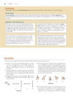
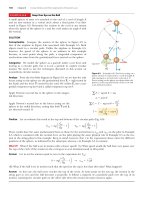
6. A crystalline solid consists of atoms stacked up in a repeating lattice structure. Consider a crystal as shown in Figure
P1.6a. The atoms reside at the corners of cubes of side
L ϭ 0.200 nm. One piece of evidence for the regular

= ThomsonNOW;

L

d
(a)

(b)
Figure P1.6

Ⅵ = symbolic reasoning;

ⅷ = qualitative reasoning


Problems

arrangement of atoms comes from the flat surfaces along
which a crystal separates, or cleaves, when it is broken.
Suppose this crystal cleaves along a face diagonal as
shown in Figure P1.6b. Calculate the spacing d between
two adjacent atomic planes that separate when the crystal
cleaves.
Section 1.3 Dimensional Analysis

7. Which of the following equations are dimensionally correct?
(a) v f ϭ vi ϩ ax (b) y ϭ (2 m) cos (kx), where k ϭ 2 mϪ1
8. Figure P1.8 shows a frustum of a cone. Of the following
mensuration (geometrical) expressions, which describes
(i) the total circumference of the flat circular faces,
(ii) the volume, and (iii) the area of the curved surface?
(a) p(r1 ϩ r2) [h2 ϩ (r2 Ϫ r1)2]1/2, (b) 2p(r1 ϩ r2)
(c) ph(r12 ϩ r1r2 ϩ r22)/3
r1

16. An ore loader moves 1 200 tons/h from a mine to the
surface. Convert this rate to pounds per second, using
1 ton ϭ 2 000 lb.
17. At the time of this book’s printing, the U.S. national debt
is about $8 trillion. (a) If payments were made at the rate
of $1 000 per second, how many years would it take to pay
off the debt, assuming no interest were charged? (b) A
dollar bill is about 15.5 cm long. If eight trillion dollar
bills were laid end to end around the Earth’s equator,
how many times would they encircle the planet? Take the
radius of the Earth at the equator to be 6 378 km. Note:
Before doing any of these calculations, try to guess at the
answers. You may be very surprised.
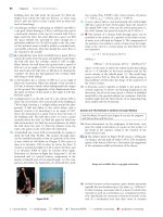
18. A pyramid has a height of 481 ft, and its base covers an
area of 13.0 acres (Fig. P1.18). The volume of a pyramid
is given by the expression V ϭ 13 Bh, where B is the area of
the base and h is the height. Find the volume of this pyramid in cubic meters. (1 acre ϭ 43 560 ft2)

Sylvain Grandadam/Photo Researchers, Inc.

h

r2
Figure P1.8

9. Newton’s law of universal gravitation is represented by
Fϭ

GMm
r2

Figure P1.18

Here F is the magnitude of the gravitational force exerted
by one small object on another, M and m are the masses
of the objects, and r is a distance. Force has the SI units
kg и m/s2. What are the SI units of the proportionality
constant G ?
Section 1.4 Conversion of Units
10. Suppose your hair grows at the rate 1/32 in. per day. Find
the rate at which it grows in nanometers per second.
Because the distance between atoms in a molecule is on
the order of 0.1 nm, your answer suggests how rapidly layers of atoms are assembled in this protein synthesis.
11. A rectangular building lot is 100 ft by 150 ft. Determine
the area of this lot in square meters.
12. An auditorium measures 40.0 m ϫ 20.0 m ϫ 12.0 m. The
density of air is 1.20 kg/m3. What are (a) the volume of
the room in cubic feet and (b) the weight of air in the
room in pounds?
13. ⅷ A room measures 3.8 m by 3.6 m, and its ceiling is

2.5 m high. Is it possible to completely wallpaper the walls
of this room with the pages of this book? Explain your
answer.
14. Assume it takes 7.00 min to fill a 30.0-gal gasoline tank.
(a) Calculate the rate at which the tank is filled in gallons
per second. (b) Calculate the rate at which the tank is
filled in cubic meters per second. (c) Determine the time
interval, in hours, required to fill a 1.00-m3 volume at the
same rate. (1 U.S. gal ϭ 231 in.3)
15. A solid piece of lead has a mass of 23.94 g and a volume
of 2.10 cm3. From these data, calculate the density of lead
in SI units (kg/m3).
2 = intermediate;

3 = challenging;

Ⅺ = SSM/SG;

ᮡ

15

Problems 18 and 19.

19. The pyramid described in Problem 18 contains approximately 2 million stone blocks that average 2.50 tons each.
Find the weight of this pyramid in pounds.
20. A hydrogen atom has a diameter of 1.06 ϫ 10Ϫ10 m as
defined by the diameter of the spherical electron cloud
around the nucleus. The hydrogen nucleus has a diameter of approximately 2.40 ϫ 10Ϫ15 m. (a) For a scale
model, represent the diameter of the hydrogen atom

by the playing length of an American football field
(100 yards ϭ 300 ft) and determine the diameter of the
nucleus in millimeters. (b) The atom is how many times
larger in volume than its nucleus?
21. ᮡ One gallon of paint (volume ϭ 3.78 ϫ 10Ϫ3 m3) covers
an area of 25.0 m2. What is the thickness of the fresh
paint on the wall?
22. The mean radius of the Earth is 6.37 ϫ 106 m and that of
the Moon is 1.74 ϫ 108 cm. From these data calculate
(a) the ratio of the Earth’s surface area to that of the
Moon and (b) the ratio of the Earth’s volume to that of
the Moon. Recall that the surface area of a sphere is 4 pr 2
and the volume of a sphere is 43 pr 3.
23. ᮡ One cubic meter (1.00 m3) of aluminum has a mass of
2.70 ϫ 103 kg, and the same volume of iron has a mass of
7.86 ϫ 103 kg. Find the radius of a solid aluminum sphere
that will balance a solid iron sphere of radius 2.00 cm on
an equal-arm balance.
24. Let rAl represent the density of aluminum and rFe that of
iron. Find the radius of a solid aluminum sphere that balances a solid iron sphere of radius rFe on an equal-arm
balance.

= ThomsonNOW;

Ⅵ = symbolic reasoning;

ⅷ = qualitative reasoning


16

Chapter 1

Physics and Measurement

Section 1.5 Estimates and Order-of-Magnitude
Calculations
25. ᮡ Find the order of magnitude of the number of tabletennis balls that would fit into a typical-size room (without
being crushed). In your solution, state the quantities you
measure or estimate and the values you take for them.
26. An automobile tire is rated to last for 50 000 miles. To an
order of magnitude, through how many revolutions will it
turn? In your solution, state the quantities you measure or
estimate and the values you take for them.
27. Compute the order of magnitude of the mass of a bathtub half full of water. Compute the order of magnitude of
the mass of a bathtub half full of pennies. In your solution, list the quantities you take as data and the value you
measure or estimate for each.
28. ⅷ Suppose Bill Gates offers to give you $1 billion if you
can finish counting it out using only one-dollar bills.
Should you accept his offer? Explain your answer. Assume
you can count one bill every second, and note that you
need at least 8 hours a day for sleeping and eating.
29. To an order of magnitude, how many piano tuners are
in New York City? Physicist Enrico Fermi was famous for
asking questions like this one on oral doctorate qualifying examinations. His own facility in making order-ofmagnitude calculations is exemplified in Problem 48 of
Chapter 45.
Section 1.6 Significant Figures
Note: Appendix B.8 on propagation of uncertainty may be
useful in solving some problems in this section.
30. A rectangular plate has a length of (21.3 Ϯ 0.2) cm and a

width of (9.8 Ϯ 0.1) cm. Calculate the area of the plate,
including its uncertainty.
31. How many significant figures are in the following numbers: (a) 78.9 Ϯ 0.2 (b) 3.788 ϫ 109 (c) 2.46 ϫ 10Ϫ6
(d) 0.005 3?
32. The radius of a uniform solid sphere is measured to
be (6.50 Ϯ 0.20) cm, and its mass is measured to be
(1.85 Ϯ 0.02) kg. Determine the density of the sphere in
kilograms per cubic meter and the uncertainty in the
density.
33. Carry out the following arithmetic operations: (a) the sum
of the measured values 756, 37.2, 0.83, and 2 (b) the
product 0.003 2 ϫ 356.3 (c) the product 5.620 ϫ p
34. The tropical year, the time interval from one vernal equinox to the next vernal equinox, is the basis for our calendar. It contains 365.242 199 days. Find the number of seconds in a tropical year.
Note: The next 11 problems call on mathematical skills that
will be useful throughout the course.
35. Review problem. A child is surprised that she must pay
$1.36 for a toy marked $1.25 because of sales tax. What is
the effective tax rate on this purchase, expressed as a percentage?
36. ⅷ Review problem. A student is supplied with a stack of
copy paper, ruler, compass, scissors, and a sensitive balance. He cuts out various shapes in various sizes, calculates their areas, measures their masses, and prepares the
graph of Figure P1.36. Consider the fourth experimental
2 = intermediate;

3 = challenging;

Ⅺ = SSM/SG;

ᮡ

point from the top. How far is it from the best-fit straight

line? (a) Express your answer as a difference in verticalaxis coordinate. (b) Express your answer as a difference
in horizontal-axis coordinate. (c) Express both of the
answers to parts (a) and (b) as a percentage. (d) Calculate the slope of the line. (e) State what the graph
demonstrates, referring to the shape of the graph and the
results of parts (c) and (d). (f) Describe whether this
result should be expected theoretically. Describe the physical meaning of the slope.
Dependence of mass on
area for paper shapes
Mass (g)
0.3
0.2
0.1

0

200

400

600

Area (cm2)
Rectangles

Squares

Circles

Triangles

Best fit

Figure P1.36

37. Review problem. A young immigrant works overtime,
earning money to buy portable MP3 players to send home
as gifts for family members. For each extra shift he works,
he has figured out that he can buy one player and twothirds of another one. An e-mail from his mother informs
him that the players are so popular that each of 15 young
neighborhood friends wants one. How many more shifts
will he have to work?
38. Review problem. In a college parking lot, the number of
ordinary cars is larger than the number of sport utility
vehicles by 94.7%. The difference between the number of
cars and the number of SUVs is 18. Find the number of
SUVs in the lot.
39. Review problem. The ratio of the number of sparrows visiting a bird feeder to the number of more interesting
birds is 2.25. On a morning when altogether 91 birds visit
the feeder, what is the number of sparrows?
40. Review problem. Prove that one solution of the equation
2.00x4 Ϫ 3.00x3 ϩ 5.00x ϭ 70.0
is x ϭ Ϫ2.22.
41. Review problem. Find every angle u between 0 and 360°
for which the ratio of sin u to cos u is Ϫ3.00.
42. Review problem. A highway curve forms a section of a circle. A car goes around the curve. Its dashboard compass
shows that the car is initially heading due east. After it travels 840 m, it is heading 35.0° south of east. Find the radius
of curvature of its path. Suggestion: You may find it useful
to learn a geometric theorem stated in Appendix B.3.
43. Review problem. For a period of time as an alligator
grows, its mass is proportional to the cube of its length.

When the alligator’s length changes by 15.8%, its mass
increases by 17.3 kg. Find its mass at the end of this
process.

= ThomsonNOW;

Ⅵ = symbolic reasoning;

ⅷ = qualitative reasoning


Problems

44. Review problem. From the set of equations
p ϭ 3q
pr ϭ qs
1
2
2 pr

ϩ

1
2
2 qs

ϭ 12 qt 2

involving the unknowns p, q, r, s, and t, find the value of
the ratio of t to r.

45. ⅷ Review problem. In a particular set of experimental trials, students examine a system described by the equation
Q
¢t

ϭ

kp d 2 1Th Ϫ Tc 2
4L

We will see this equation and the various quantities in it
in Chapter 20. For experimental control, in these trials all
quantities except d and ⌬t are constant. (a) If d is made
three times larger, does the equation predict that ⌬t will
get larger or smaller? By what factor? (b) What pattern of
proportionality of ⌬t to d does the equation predict? (c) To
display this proportionality as a straight line on a graph,
what quantities should you plot on the horizontal and vertical axes? (d) What expression represents the theoretical
slope of this graph?
Additional Problems
46. In a situation in which data are known to three significant
digits, we write 6.379 m ϭ 6.38 m and 6.374 m ϭ 6.37 m.
When a number ends in 5, we arbitrarily choose to write
6.375 m ϭ 6.38 m. We could equally well write 6.375 m ϭ
6.37 m, “rounding down” instead of “rounding up,”
because we would change the number 6.375 by equal
increments in both cases. Now consider an order-ofmagnitude estimate, in which factors of change rather
than increments are important. We write 500 m ϳ 103 m
because 500 differs from 100 by a factor of 5, whereas it
differs from 1 000 by only a factor of 2. We write 437 m ϳ
103 m and 305 m ϳ 102 m. What distance differs from

100 m and from 1 000 m by equal factors so that we could
equally well choose to represent its order of magnitude
either as ϳ102 m or as ϳ103 m?
47. ⅷ A spherical shell has an outside radius of 2.60 cm and
an inside radius of a. The shell wall has uniform thickness
and is made of a material with density 4.70 g/cm3. The
space inside the shell is filled with a liquid having a density
of 1.23 g/cm3. (a) Find the mass m of the sphere, including its contents, as a function of a. (b) In the answer to
part (a), if a is regarded as a variable, for what value of a
does m have its maximum possible value? (c) What is this
maximum mass? (d) Does the value from part (b) agree
with the result of a direct calculation of the mass of a
sphere of uniform density? (e) For what value of a does
the answer to part (a) have its minimum possible value?
(f) What is this minimum mass? (g) Does the value from
part (f) agree with the result of a direct calculation of the
mass of a uniform sphere? (h) What value of m is halfway
between the maximum and minimum possible values?
(i) Does this mass agree with the result of part (a) evaluated for a ϭ 2.60 cm/2 ϭ 1.30 cm? (j) Explain whether
you should expect agreement in each of parts (d), (g),
and (i). (k) What If? In part (a), would the answer
change if the inner wall of the shell were not concentric
with the outer wall?
2 = intermediate;

3 = challenging;

Ⅺ = SSM/SG;

ᮡ

17

48. A rod extending between x ϭ 0 and x ϭ 14.0 cm has uniform cross-sectional area A ϭ 9.00 cm2. It is made from a
continuously changing alloy of metals so that along its
length its density changes steadily from 2.70 g/cm3 to
19.3 g/cm3. (a) Identify the constants B and C required in
the expression r ϭ B ϩ Cx to describe the variable density. (b) The mass of the rod is given by
14 cm

mϭ

Ύ rdV ϭ Ύ rAdx ϭ Ύ 1B ϩ Cx 2 19.00 cm 2 dx

all material

2

all x

0

Carry out the integration to find the mass of the rod.
49. The diameter of our disk-shaped galaxy, the Milky Way, is
about 1.0 ϫ 105 light-years (ly). The distance to Andromeda, which is the spiral galaxy nearest to the Milky Way, is
about 2.0 million ly. If a scale model represents the Milky
Way and Andromeda galaxies as dinner plates 25 cm in
diameter, determine the distance between the centers of
the two plates.
50. ⅷ Air is blown into a spherical balloon so that, when its

radius is 6.50 cm, its radius is increasing at the rate
0.900 cm/s. (a) Find the rate at which the volume of the
balloon is increasing. (b) If this volume flow rate of air
entering the balloon is constant, at what rate will the
radius be increasing when the radius is 13.0 cm?
(c) Explain physically why the answer to part (b) is larger
or smaller than 0.9 cm/s, if it is different.
51. ᮡ The consumption of natural gas by a company satisfies
the empirical equation V ϭ 1.50t ϩ 0.008 00t 2, where V is
the volume in millions of cubic feet and t is the time in
months. Express this equation in units of cubic feet and
seconds. Assign proper units to the coefficients. Assume a
month is 30.0 days.
52.
In physics it is important to use mathematical approximations. Demonstrate that for small angles (Ͻ 20°),
tan a Ϸ sin a Ϸ a ϭ

pa¿
180°

where a is in radians and aЈ is in degrees. Use a calculator to find the largest angle for which tan a may be
approximated by a with an error less than 10.0%.
53. A high fountain of water is located at the center of a circular pool as shown in Figure P1.53. Not wishing to get
his feet wet, a student walks around the pool and measures its circumference to be 15.0 m. Next, the student
stands at the edge of the pool and uses a protractor to
gauge the angle of elevation of the top of the fountain to
be 55.0°. How high is the fountain?

55.0Њ

Figure P1.53

54. ⅷ Collectible coins are sometimes plated with gold to
enhance their beauty and value. Consider a commemorative quarter-dollar advertised for sale at $4.98. It has a

= ThomsonNOW;

Ⅵ = symbolic reasoning;

ⅷ = qualitative reasoning


18

Chapter 1

Physics and Measurement

diameter of 24.1 mm and a thickness of 1.78 mm, and it is
completely covered with a layer of pure gold 0.180 mm
thick. The volume of the plating is equal to the thickness
of the layer times the area to which it is applied. The patterns on the faces of the coin and the grooves on its edge
have a negligible effect on its area. Assume the price of
gold is $10.0 per gram. Find the cost of the gold added to
the coin. Does the cost of the gold significantly enhance
the value of the coin? Explain your answer.
55. One year is nearly p ϫ 107 s. Find the percentage error in
this approximation, where “percentage error” is defined as
Percentage error ϭ

0 assumed value Ϫ true value 0
true value

ϫ 100%

56. ⅷ A creature moves at a speed of 5.00 furlongs per fortnight (not a very common unit of speed). Given that
1 furlong ϭ 220 yards and 1 fortnight ϭ 14 days, determine the speed of the creature in meters per second.
Explain what kind of creature you think it might be.
57. A child loves to watch as you fill a transparent plastic bottle with shampoo. Horizontal cross sections of the bottle
are circles with varying diameters because the bottle is
much wider in some places than others. You pour in
bright green shampoo with constant volume flow rate
16.5 cm3/s. At what rate is its level in the bottle rising
(a) at a point where the diameter of the bottle is 6.30 cm
and (b) at a point where the diameter is 1.35 cm?

58. ⅷ The data in the following table represent measurements of the masses and dimensions of solid cylinders of
aluminum, copper, brass, tin, and iron. Use these data to
calculate the densities of these substances. State how your
results for aluminum, copper, and iron compare with
those given in Table 14.1.
Substance

Mass
(g)

Diameter
(cm)

Length

(cm)

Aluminum
Copper
Brass
Tin
Iron

51.5
56.3
94.4
69.1
216.1

2.52
1.23
1.54
1.75
1.89

3.75
5.06
5.69
3.74
9.77

59. Assume there are 100 million passenger cars in the United
States and the average fuel consumption is 20 mi/gal of
gasoline. If the average distance traveled by each car is
10 000 mi/yr, how much gasoline would be saved per year

if average fuel consumption could be increased to
25 mi/gal?
60. The distance from the Sun to the nearest star is about
4 ϫ 1016 m. The Milky Way galaxy is roughly a disk of
diameter ϳ1021 m and thickness ϳ1019 m. Find the order
of magnitude of the number of stars in the Milky Way.
Assume the distance between the Sun and our nearest
neighbor is typical.

Answers to Quick Quizzes
1.1 (a). Because the density of aluminum is smaller than that
of iron, a larger volume of aluminum than iron is
required for a given mass.
1.2 False. Dimensional analysis gives the units of the proportionality constant but provides no information about its
numerical value. To determine its numerical value
requires either experimental data or geometrical reason-

2 = intermediate;

3 = challenging;

Ⅺ = SSM/SG;

ᮡ

ing. For example, in the generation of the equation x ϭ
1
1 2
2 at , because the factor 2 is dimensionless there is no way
to determine it using dimensional analysis.

1.3 (b). Because there are 1.609 km in 1 mi, a larger number
of kilometers than miles is required for a given distance.

= ThomsonNOW;

Ⅵ = symbolic reasoning;

ⅷ = qualitative reasoning


2.1

Position, Velocity, and
Speed

2.6

The Particle Under
Constant Acceleration

2.2

Instantaneous Velocity
and Speed

2.7

Freely Falling Objects

2.8

Kinematic Equations
Derived from Calculus

2.3

Analysis Models: The
Particle Under Constant
Velocity

2.4

Acceleration

2.5

Motion Diagrams

General ProblemSolving Strategy

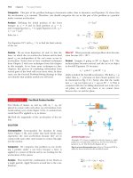
In drag racing, a driver wants as large an acceleration as possible. In a distance of one-quarter mile, a vehicle reaches speeds of more than 320 mi/h,
covering the entire distance in under 5 s. (George Lepp/Stone/Getty)

2

Motion in One Dimension

As a first step in studying classical mechanics, we describe the motion of an object
while ignoring the interactions with external agents that might be causing or modifying that motion. This portion of classical mechanics is called kinematics. (The word
kinematics has the same root as cinema. Can you see why?) In this chapter, we consider

only motion in one dimension, that is, motion of an object along a straight line.
From everyday experience we recognize that motion of an object represents a
continuous change in the object’s position. In physics, we can categorize motion
into three types: translational, rotational, and vibrational. A car traveling on a
highway is an example of translational motion, the Earth’s spin on its axis is an
example of rotational motion, and the back-and-forth movement of a pendulum is
an example of vibrational motion. In this and the next few chapters, we are concerned only with translational motion. (Later in the book we shall discuss rotational and vibrational motions.)
In our study of translational motion, we use what is called the particle model
and describe the moving object as a particle regardless of its size. In general, a particle is a point-like object, that is, an object that has mass but is of infinitesimal
size. For example, if we wish to describe the motion of the Earth around the Sun,
we can treat the Earth as a particle and obtain reasonably accurate data about its
orbit. This approximation is justified because the radius of the Earth’s orbit is
large compared with the dimensions of the Earth and the Sun. As an example on
19


20

Chapter 2

Motion in One Dimension

a much smaller scale, it is possible to explain the pressure exerted by a gas on the
walls of a container by treating the gas molecules as particles, without regard for
the internal structure of the molecules.

2.1

The motion of a particle is completely known if the particle’s position in space is
known at all times. A particle’s position is the location of the particle with respect

to a chosen reference point that we can consider to be the origin of a coordinate
system.
Consider a car moving back and forth along the x axis as in Active Figure 2.1a.
When we begin collecting position data, the car is 30 m to the right of a road sign,
which we will use to identify the reference position x ϭ 0. We will use the particle
model by identifying some point on the car, perhaps the front door handle, as a
particle representing the entire car.
We start our clock, and once every 10 s we note the car’s position relative to the
sign at x ϭ 0. As you can see from Table 2.1, the car moves to the right (which we
have defined as the positive direction) during the first 10 s of motion, from position Ꭽ to position Ꭾ. After Ꭾ, the position values begin to decrease, suggesting
the car is backing up from position Ꭾ through position ൵. In fact, at ൳, 30 s after
we start measuring, the car is alongside the road sign that we are using to mark
our origin of coordinates (see Active Figure 2.1a). It continues moving to the left
and is more than 50 m to the left of the sign when we stop recording information
after our sixth data point. A graphical representation of this information is presented in Active Figure 2.1b. Such a plot is called a position–time graph.
Notice the alternative representations of information that we have used for the
motion of the car. Active Figure 2.1a is a pictorial representation, whereas Active Figure 2.1b is a graphical representation. Table 2.1 is a tabular representation of the same
information. Using an alternative representation is often an excellent strategy for
understanding the situation in a given problem. The ultimate goal in many problems is a mathematical representation, which can be analyzed to solve for some
requested piece of information.

ᮣ

Position

TABLE 2.1
Position of the Car
at Various Times
Position

t (s)

x (m)

0
10
20
30
40
50

30
52
38
0
Ϫ37
Ϫ53

Ꭽ
Ꭾ
Ꭿ
൳
൴
൵

Position, Velocity, and Speed

x (m)
60

Ꭾ
⌬x

40
Ϫ60
Ϫ50
Ϫ40Ϫ30
Ϫ20Ϫ10

൵

IT
L IM
/h
30km

0

൴

Ϫ60
Ϫ50
Ϫ40
Ϫ30Ϫ20
Ϫ10

10

20

Ꭽ
Ꭽ
30 40

20

50 60
x (m)

Ꭿ

(a)

20

30 40

൳

0

IT

10

⌬t

Ꭾ

൳ 3L0IMkm/h

0

Ꭿ

50 60
x (m)

Ϫ20

൴

Ϫ40
Ϫ60
0

൵
t (s)
10

20

30

40

50

(b)

ACTIVE FIGURE 2.1

A car moves back and forth along a straight line. Because we are interested only in the car’s translational
motion, we can model it as a particle. Several representations of the information about the motion of
the car can be used. Table 2.1 is a tabular representation of the information. (a) A pictorial representation of the motion of the car. (b) A graphical representation (position–time graph) of the motion of
the car.
Sign in at www.thomsonedu.com and go to ThomsonNOW to move each of the six points Ꭽ through ൵
and observe the motion of the car in both a pictorial and a graphical representation as it follows a
smooth path through the six points.


Section 2.1

Position, Velocity, and Speed

21

Given the data in Table 2.1, we can easily determine the change in position of
the car for various time intervals. The displacement of a particle is defined as its
change in position in some time interval. As the particle moves from an initial
position xi to a final position xf , its displacement is given by
¢x ϵ xf Ϫ xi

(2.1)

ᮤ

Displacement

We use the capital Greek letter delta (⌬) to denote the change in a quantity. From
this definition we see that ⌬x is positive if xf is greater than xi and negative if xf is
less than xi.

It is very important to recognize the difference between displacement and distance traveled. Distance is the length of a path followed by a particle. Consider, for Image not available due to copyright restrictions
example, the basketball players in Figure 2.2. If a player runs from his own team’s
basket down the court to the other team’s basket and then returns to his own basket, the displacement of the player during this time interval is zero because he
ended up at the same point as he started: xf ϭ xi , so ⌬x ϭ 0. During this time interval, however, he moved through a distance of twice the length of the basketball
court. Distance is always represented as a positive number, whereas displacement
can be either positive or negative.
Displacement is an example of a vector quantity. Many other physical quantities,
including position, velocity, and acceleration, also are vectors. In general, a vector
quantity requires the specification of both direction and magnitude. By contrast, a
scalar quantity has a numerical value and no direction. In this chapter, we use positive (ϩ) and negative (Ϫ) signs to indicate vector direction. For example, for horizontal motion let us arbitrarily specify to the right as being the positive direction.
It follows that any object always moving to the right undergoes a positive displacement ⌬x Ͼ 0, and any object moving to the left undergoes a negative displacement
so that ⌬x Ͻ 0. We shall treat vector quantities in greater detail in Chapter 3.
One very important point has not yet been mentioned. Notice that the data in
Table 2.1 result only in the six data points in the graph in Active Figure 2.1b. The
smooth curve drawn through the six points in the graph is only a possibility of the
actual motion of the car. We only have information about six instants of time; we
have no idea what happened in between the data points. The smooth curve is a
guess as to what happened, but keep in mind that it is only a guess.
If the smooth curve does represent the actual motion of the car, the graph contains information about the entire 50-s interval during which we watch the car
move. It is much easier to see changes in position from the graph than from a verbal description or even a table of numbers. For example, it is clear that the car
covers more ground during the middle of the 50-s interval than at the end.
Between positions Ꭿ and ൳, the car travels almost 40 m, but during the last 10 s,
between positions ൴ and ൵, it moves less than half that far. A common way of
comparing these different motions is to divide the displacement ⌬x that occurs
between two clock readings by the value of that particular time interval ⌬t. The
result turns out to be a very useful ratio, one that we shall use many times. This
ratio has been given a special name: the average velocity. The average velocity vx, avg
of a particle is defined as the particle’s displacement ⌬x divided by the time interval ⌬t during which that displacement occurs:
vx,¬avg ϵ

¢x
¢t

(2.2)

where the subscript x indicates motion along the x axis. From this definition we
see that average velocity has dimensions of length divided by time (L/T), or
meters per second in SI units.
The average velocity of a particle moving in one dimension can be positive or
negative, depending on the sign of the displacement. (The time interval ⌬t is always
positive.) If the coordinate of the particle increases in time (that is, if xf Ͼ xi), ⌬x is
positive and vx, avg ϭ ⌬x/⌬t is positive. This case corresponds to a particle moving in
the positive x direction, that is, toward larger values of x. If the coordinate decreases

ᮤ

Average velocity


22

Chapter 2

Motion in One Dimension

in time (that is, if xf Ͻ xi), ⌬x is negative and hence vx, avg is negative. This case corresponds to a particle moving in the negative x direction.
We can interpret average velocity geometrically by drawing a straight line
between any two points on the position–time graph in Active Figure 2.1b. This line
forms the hypotenuse of a right triangle of height ⌬x and base ⌬t. The slope of
this line is the ratio ⌬x/⌬t, which is what we have defined as average velocity in

Equation 2.2. For example, the line between positions Ꭽ and Ꭾ in Active Figure
2.1b has a slope equal to the average velocity of the car between those two times,
(52 m Ϫ 30 m)/(10 s Ϫ 0) ϭ 2.2 m/s.
In everyday usage, the terms speed and velocity are interchangeable. In physics,
however, there is a clear distinction between these two quantities. Consider a
marathon runner who runs a distance d of more than 40 km and yet ends up at
her starting point. Her total displacement is zero, so her average velocity is zero!
Nonetheless, we need to be able to quantify how fast she was running. A slightly
different ratio accomplishes that for us. The average speed vavg of a particle, a
scalar quantity, is defined as the total distance traveled divided by the total time
interval required to travel that distance:
Average speed

vavg ϵ

ᮣ

PITFALL PREVENTION 2.1
Average Speed and Average Velocity
The magnitude of the average
velocity is not the average speed.
For example, consider the
marathon runner discussed before
Equation 2.3. The magnitude of
her average velocity is zero, but her
average speed is clearly not zero.

d
¢t

(2.3)

The SI unit of average speed is the same as the unit of average velocity: meters per
second. Unlike average velocity, however, average speed has no direction and is
always expressed as a positive number. Notice the clear distinction between the
definitions of average velocity and average speed: average velocity (Eq. 2.2) is the
displacement divided by the time interval, whereas average speed (Eq. 2.3) is the distance divided by the time interval.
Knowledge of the average velocity or average speed of a particle does not provide information about the details of the trip. For example, suppose it takes you
45.0 s to travel 100 m down a long, straight hallway toward your departure gate at
an airport. At the 100-m mark, you realize you missed the restroom, and you
return back 25.0 m along the same hallway, taking 10.0 s to make the return trip.
The magnitude of your average velocity is ϩ75.0 m/55.0 s ϭ ϩ1.36 m/s. The average speed for your trip is 125 m/55.0 s ϭ 2.27 m/s. You may have traveled at various speeds during the walk. Neither average velocity nor average speed provides
information about these details.

Quick Quiz 2.1 Under which of the following conditions is the magnitude of
the average velocity of a particle moving in one dimension smaller than the average speed over some time interval? (a) a particle moves in the ϩx direction without reversing (b) a particle moves in the Ϫx direction without reversing (c) a
particle moves in the ϩx direction and then reverses the direction of its motion
(d) there are no conditions for which this is true

E XA M P L E 2 . 1

Calculating the Average Velocity and Speed

Find the displacement, average velocity, and average speed of the car in Active Figure 2.1a between positions Ꭽ and ൵.
SOLUTION
Consult Active Figure 2.1 to form a mental image of the car and its motion. We model the car as a particle. From the
position–time graph given in Active Figure 2.1b, notice that xᎭ ϭ 30 m at tᎭ ϭ 0 s and that x൵ ϭ Ϫ53 m at t൵ ϭ 50 s.
Use Equation 2.1 to find the displacement of the car:

⌬x ϭ x൵ Ϫ xᎭ ϭ Ϫ53 m Ϫ 30 m ϭ Ϫ83 m

This result means that the car ends up 83 m in the negative direction (to the left, in this case) from where it started.
This number has the correct units and is of the same order of magnitude as the supplied data. A quick look at Active
Figure 2.1a indicates that it is the correct answer.


Section 2.2

v x, avg ϭ

Use Equation 2.2 to find the average velocity:

ϭ

Instantaneous Velocity and Speed

23

x൵ Ϫ xᎭ
t൵ Ϫ tᎭ
Ϫ53 m Ϫ 30 m
Ϫ83 m
ϭ
ϭ Ϫ1.7 m>s
50 s Ϫ 0 s
50 s

We cannot unambiguously find the average speed of the car from the data in Table 2.1 because we do not have information about the positions of the car between the data points. If we adopt the assumption that the details of the
car’s position are described by the curve in Active Figure 2.1b, the distance traveled is 22 m (from Ꭽ to Ꭾ) plus 105 m
(from Ꭾ to ൵), for a total of 127 m.

vavg ϭ

Use Equation 2.3 to find the car’s average speed:

127 m
ϭ 2.5 m>s
50 s

Notice that the average speed is positive, as it must be. Suppose the brown curve in Active Figure 2.1b were different
so that between 0 s and 10 s it went from Ꭽ up to 100 m and then came back down to Ꭾ. The average speed of the
car would change because the distance is different, but the average velocity would not change.

2.2

Instantaneous Velocity and Speed

Often we need to know the velocity of a particle at a particular instant in time
rather than the average velocity over a finite time interval. In other words, you
would like to be able to specify your velocity just as precisely as you can specify
your position by noting what is happening at a specific clock reading—that is, at
some specific instant. What does it mean to talk about how quickly something is
moving if we “freeze time” and talk only about an individual instant? In the late
1600s, with the invention of calculus, scientists began to understand how to
describe an object’s motion at any moment in time.
To see how that is done, consider Active Figure 2.3a, which is a reproduction of
the graph in Active Figure 2.1b. We have already discussed the average velocity for
the interval during which the car moved from position Ꭽ to position Ꭾ (given by
the slope of the blue line) and for the interval during which it moved from Ꭽ to
൵ (represented by the slope of the longer blue line and calculated in Example
2.1). The car starts out by moving to the right, which we defined to be the positive

direction. Therefore, being positive, the value of the average velocity during the
interval from Ꭽ to Ꭾ is more representative of the initial velocity than is the value

60

x (m)

Ꭾ

60
Ꭿ

40

Ꭽ

Ꭾ

20

൳

0

40

Ϫ20

൴

Ϫ40
Ϫ60

Ꭾ Ꭾ Ꭾ

0

10

20

30
(a)

40

൵
t (s)
50

Ꭽ
(b)

ACTIVE FIGURE 2.3
(a) Graph representing the motion of the car in Active Figure 2.1. (b) An enlargement of the upper-lefthand corner of the graph shows how the blue line between positions Ꭽ and Ꭾ approaches the green
tangent line as point Ꭾ is moved closer to point Ꭽ.
Sign in at www.thomsonedu.com and go to ThomsonNOW to move point Ꭾ as suggested in part (b) and
observe the blue line approaching the green tangent line.

PITFALL PREVENTION 2.2

Slopes of Graphs
In any graph of physical data, the
slope represents the ratio of the
change in the quantity represented
on the vertical axis to the change
in the quantity represented on the
horizontal axis. Remember that a
slope has units (unless both axes
have the same units). The units of
slope in Active Figure 2.1b and
Active Figure 2.3 are meters per
second, the units of velocity.


24

Chapter 2

Motion in One Dimension

of the average velocity during the interval from Ꭽ to ൵, which we determined to
be negative in Example 2.1. Now let us focus on the short blue line and slide point
Ꭾ to the left along the curve, toward point Ꭽ, as in Active Figure 2.3b. The line
between the points becomes steeper and steeper, and as the two points become
extremely close together, the line becomes a tangent line to the curve, indicated
by the green line in Active Figure 2.3b. The slope of this tangent line represents
the velocity of the car at point Ꭽ. What we have done is determine the instantaneous velocity at that moment. In other words, the instantaneous velocity vx equals
the limiting value of the ratio ⌬x/⌬t as ⌬t approaches zero:1
¢x
¢tS0 ¢t

vx ϵ lim

Instantaneous velocity

ᮣ

PITFALL PREVENTION 2.3
Instantaneous Speed and Instantaneous Velocity
In Pitfall Prevention 2.1, we argued
that the magnitude of the average
velocity is not the average speed.
The magnitude of the instantaneous velocity, however, is the
instantaneous speed. In an infinitesimal time interval, the magnitude of the displacement is equal
to the distance traveled by the
particle.

(2.4)

In calculus notation, this limit is called the derivative of x with respect to t, written
dx/dt:
¢x
dx
ϭ
vx ϵ lim
(2.5)
¢t
dt
¢tS0
The instantaneous velocity can be positive, negative, or zero. When the slope of

the position–time graph is positive, such as at any time during the first 10 s in
Active Figure 2.3, vx is positive and the car is moving toward larger values of x.
After point Ꭾ, vx is negative because the slope is negative and the car is moving
toward smaller values of x. At point Ꭾ, the slope and the instantaneous velocity
are zero and the car is momentarily at rest.
From here on, we use the word velocity to designate instantaneous velocity.
When we are interested in average velocity, we shall always use the adjective average.
The instantaneous speed of a particle is defined as the magnitude of its instantaneous velocity. As with average speed, instantaneous speed has no direction
associated with it. For example, if one particle has an instantaneous velocity of
ϩ25 m/s along a given line and another particle has an instantaneous velocity of
Ϫ25 m/s along the same line, both have a speed2 of 25 m/s.

Quick Quiz 2.2

Are members of the highway patrol more interested in (a) your
average speed or (b) your instantaneous speed as you drive?

CO N C E P T UA L E XA M P L E 2 . 2

The Velocity of Different Objects

Consider the following one-dimensional motions: (A) a
ball thrown directly upward rises to a highest point and
falls back into the thrower’s hand; (B) a race car starts
from rest and speeds up to 100 m/s; and (C) a spacecraft drifts through space at constant velocity. Are there
any points in the motion of these objects at which the
instantaneous velocity has the same value as the average
velocity over the entire motion? If so, identify the
point(s).

its displacement is zero. There is one point at which the
instantaneous velocity is zero: at the top of the motion.

SOLUTION
(A) The average velocity for the thrown ball is zero
because the ball returns to the starting point; therefore,

(C) Because the spacecraft’s instantaneous velocity is
constant, its instantaneous velocity at any time and its
average velocity over any time interval are the same.

(B) The car’s average velocity cannot be evaluated
unambiguously with the information given, but it must
have some value between 0 and 100 m/s. Because the
car will have every instantaneous velocity between 0 and
100 m/s at some time during the interval, there must be
some instant at which the instantaneous velocity is equal
to the average velocity over the entire motion.

Notice that the displacement ⌬x also approaches zero as ⌬t approaches zero, so the ratio looks like
0/0. As ⌬x and ⌬t become smaller and smaller, the ratio ⌬x/⌬t approaches a value equal to the slope of
the line tangent to the x-versus-t curve.

1

2

As with velocity, we drop the adjective for instantaneous speed. “Speed” means instantaneous speed.

Section 2.2

E XA M P L E 2 . 3

25

Instantaneous Velocity and Speed

Average and Instantaneous Velocity

A particle moves along the x axis. Its position varies with time according to
the expression x ϭ Ϫ4t ϩ 2t 2, where x is in meters and t is in seconds.3 The
position–time graph for this motion is shown in Figure 2.4. Notice that the
particle moves in the negative x direction for the first second of motion, is
momentarily at rest at the moment t ϭ 1 s, and moves in the positive x
direction at times t Ͼ 1 s.

x (m)
10
8
6

(A) Determine the displacement of the particle in the time intervals t ϭ 0 to
t ϭ 1 s and t ϭ 1 s to t ϭ 3 s.
SOLUTION
From the graph in Figure 2.4, form a mental representation of the motion
of the particle. Keep in mind that the particle does not move in a curved
path in space such as that shown by the brown curve in the graphical representation. The particle moves only along the x axis in one dimension. At
t ϭ 0, is it moving to the right or to the left?
During the first time interval, the slope is negative and hence the average

velocity is negative. Therefore, we know that the displacement between Ꭽ
and Ꭾ must be a negative number having units of meters. Similarly, we
expect the displacement between Ꭾ and ൳ to be positive.

Slope ϭ Ϫ2 m/s

2
0

Ꭿ

Ꭽ

t (s)

Ϫ2
Ϫ4

൳

Slope ϭ ϩ4 m/s

4

Ꭾ
0

1

2

3

4

Figure 2.4 (Example 2.3) Position–time
graph for a particle having an x coordinate that varies in time according to the
expression x ϭ Ϫ4t ϩ 2t 2.

In the first time interval, set ti ϭ tᎭ ϭ 0 and tf ϭ tᎮ ϭ 1 s
and use Equation 2.1 to find the displacement:

⌬xᎭSᎮ ϭ xf Ϫ xi ϭ xᎮ Ϫ xᎭ

For the second time interval (t ϭ 1 s to t ϭ 3 s), set ti ϭ
tᎮ ϭ 1 s and tf ϭ t൳ ϭ 3 s:

⌬xᎮS൳ ϭ xf Ϫ xi ϭ x൳ Ϫ xᎮ

ϭ 3Ϫ4 11 2 ϩ 2 112 2 4 Ϫ 3Ϫ4 102 ϩ 2 102 2 4 ϭ Ϫ2 m

ϭ 3Ϫ4 13 2 ϩ 2 13 2 2 4 Ϫ 3Ϫ4 112 ϩ 2 112 2 4 ϭ ϩ8 m

These displacements can also be read directly from the position–time graph.
(B) Calculate the average velocity during these two time intervals.
SOLUTION
In the first time interval, use Equation 2.2 with ⌬t ϭ tf Ϫ ti
ϭ tᎮ Ϫ tᎭ ϭ 1 s:
In the second time interval, ⌬t ϭ 2 s:

v x, avg 1ᎭSᎮ2 ϭ

¢x ᎭSᎮ

v x, avg 1ᎮS൳2 ϭ

¢t

ϭ

¢x ᎮS൳
¢t

Ϫ2 m
ϭ Ϫ2 m>s
1s

ϭ

8m
ϭ ϩ4 m>s
2s

These values are the same as the slopes of the lines joining these points in Figure 2.4.
(C) Find the instantaneous velocity of the particle at t ϭ 2.5 s.
SOLUTION
Measure the slope of the green line at t ϭ 2.5 s (point
Ꭿ) in Figure 2.4:

vx ϭ ϩ6 m>s

Notice that this instantaneous velocity is on the same order of magnitude as our previous results, that is, a few
meters per second. Is that what you would have expected?
3 Simply to make it easier to read, we write the expression as x ϭ Ϫ4t ϩ 2t 2 rather than as x ϭ (Ϫ4.00 m/s)t ϩ (2.00 m/s2)t 2.00. When an equation
summarizes measurements, consider its coefficients to have as many significant digits as other data quoted in a problem. Consider its coefficients
to have the units required for dimensional consistency. When we start our clocks at t ϭ 0, we usually do not mean to limit the precision to a single
digit. Consider any zero value in this book to have as many significant figures as you need.


26

Chapter 2

Motion in One Dimension

2.3

Analysis Models: The Particle
Under Constant Velocity

An important technique in the solution to physics problems is the use of analysis
models. Such models help us analyze common situations in physics problems and
guide us toward a solution. An analysis model is a problem we have solved before.
It is a description of either (1) the behavior of some physical entity or (2) the
interaction between that entity and the environment. When you encounter a new
problem, you should identify the fundamental details of the problem and attempt
to recognize which of the types of problems you have already solved might be used
as a model for the new problem. For example, suppose an automobile is moving
along a straight freeway at a constant speed. Is it important that it is an automobile? Is it important that it is a freeway? If the answers to both questions are no, we
model the automobile as a particle under constant velocity, which we will discuss in

this section.
This method is somewhat similar to the common practice in the legal profession of finding “legal precedents.” If a previously resolved case can be found that
is very similar legally to the current one, it is offered as a model and an argument
is made in court to link them logically. The finding in the previous case can then
be used to sway the finding in the current case. We will do something similar in
physics. For a given problem, we search for a “physics precedent,” a model with
which we are already familiar and that can be applied to the current problem.
We shall generate analysis models based on four fundamental simplification
models. The first is the particle model discussed in the introduction to this chapter. We will look at a particle under various behaviors and environmental interactions. Further analysis models are introduced in later chapters based on simplification models of a system, a rigid object, and a wave. Once we have introduced these
analysis models, we shall see that they appear again and again in different problem
situations.
Let us use Equation 2.2 to build our first analysis model for solving problems.
We imagine a particle moving with a constant velocity. The particle under constant
velocity model can be applied in any situation in which an entity that can be modeled as a particle is moving with constant velocity. This situation occurs frequently,
so this model is important.
If the velocity of a particle is constant, its instantaneous velocity at any instant
during a time interval is the same as the average velocity over the interval. That is,
vx ϭ vx, avg. Therefore, Equation 2.2 gives us an equation to be used in the mathematical representation of this situation:

x

vx ϭ
xi

⌬x
Slope ϭ
ϭ vx
⌬t

¢x

¢t

(2.6)

Remembering that ⌬x ϭ xf Ϫ xi, we see that vx ϭ (xf Ϫ xi)/⌬t, or
xf ϭ xi ϩ vx ¢t

t
Figure 2.5 Position–time graph for
a particle under constant velocity.
The value of the constant velocity is
the slope of the line.

Position as a function
of time

ᮣ

This equation tells us that the position of the particle is given by the sum of its
original position xi at time t ϭ 0 plus the displacement vx ⌬t that occurs during the
time interval ⌬t. In practice, we usually choose the time at the beginning of the
interval to be ti ϭ 0 and the time at the end of the interval to be tf ϭ t, so our
equation becomes
xf ϭ xi ϩ vxt¬1for constant vx 2

(2.7)

Equations 2.6 and 2.7 are the primary equations used in the model of a particle
under constant velocity. They can be applied to particles or objects that can be
modeled as particles.

Figure 2.5 is a graphical representation of the particle under constant velocity.
On this position–time graph, the slope of the line representing the motion is constant and equal to the magnitude of the velocity. Equation 2.7, which is the equation of a straight line, is the mathematical representation of the particle under


Section 2.4

Acceleration

27

constant velocity model. The slope of the straight line is vx and the y intercept is xi
in both representations.

E XA M P L E 2 . 4

Modeling a Runner as a Particle

A scientist is studying the biomechanics of the human body. She determines the velocity of an experimental subject
while he runs along a straight line at a constant rate. The scientist starts the stopwatch at the moment the runner
passes a given point and stops it after the runner has passed another point 20 m away. The time interval indicated on
the stopwatch is 4.0 s.
(A) What is the runner’s velocity?
SOLUTION
Think about the moving runner. We model the runner as a particle because the size of the runner and the movement of arms and legs are unnecessary details. Because the problem states that the subject runs at a constant rate, we
can model him as a particle under constant velocity.
Use Equation 2.6 to find the constant velocity of the
runner:

vx ϭ

xf Ϫ xi
¢x
20 m Ϫ 0
ϭ
ϭ
ϭ 5.0 m>s
¢t
¢t
4.0 s

(B) If the runner continues his motion after the stopwatch is stopped, what is his position after 10 s has passed?
SOLUTION
Use Equation 2.7 and the velocity found in part (A) to
find the position of the particle at time t ϭ 10 s:

xf ϭ xi ϩ vxt ϭ 0 ϩ 15.0 m>s2 110 s2 ϭ 50 m

Notice that this value is more than twice that of the 20-m position at which the stopwatch was stopped. Is this value
consistent with the time of 10 s being more than twice the time of 4.0 s?

The mathematical manipulations for the particle under constant velocity stem
from Equation 2.6 and its descendent, Equation 2.7. These equations can be used
to solve for any variable in the equations that happens to be unknown if the other
variables are known. For example, in part (B) of Example 2.4, we find the position
when the velocity and the time are known. Similarly, if we know the velocity and
the final position, we could use Equation 2.7 to find the time at which the runner
is at this position.
A particle under constant velocity moves with a constant speed along a straight
line. Now consider a particle moving with a constant speed along a curved path.
This situation can be represented with the particle under constant speed model.

The primary equation for this model is Equation 2.3, with the average speed vavg
replaced by the constant speed v:
vϭ

d
¢t

(2.8)

As an example, imagine a particle moving at a constant speed in a circular path. If
the speed is 5.00 m/s and the radius of the path is 10.0 m, we can calculate the
time interval required to complete one trip around the circle:
vϭ

2.4

d
¢t

S

¢t ϭ

2p 110.0 m2
d
2pr
ϭ
ϭ
ϭ 12.6 s
v

v
5.00 m>s

Acceleration

In Example 2.3, we worked with a common situation in which the velocity of a particle changes while the particle is moving. When the velocity of a particle changes
with time, the particle is said to be accelerating. For example, the magnitude of the
velocity of a car increases when you step on the gas and decreases when you apply
the brakes. Let us see how to quantify acceleration.


28

Chapter 2

Motion in One Dimension

Suppose an object that can be modeled as a particle moving along the x axis
has an initial velocity vxi at time ti and a final velocity vxf at time tf , as in Figure 2.6a.
The average acceleration ax, avg of the particle is defined as the change in velocity
⌬vx divided by the time interval ⌬t during which that change occurs:
Average acceleration

ax,¬avg ϵ

ᮣ

vxf Ϫ vxi
¢vx
ϭ

¢t
tf Ϫ ti

(2.9)

As with velocity, when the motion being analyzed is one dimensional, we can use
positive and negative signs to indicate the direction of the acceleration. Because the
dimensions of velocity are L/T and the dimension of time is T, acceleration has
dimensions of length divided by time squared, or L/T2. The SI unit of acceleration
is meters per second squared (m/s2). It might be easier to interpret these units if
you think of them as meters per second per second. For example, suppose an
object has an acceleration of ϩ2 m/s2. You should form a mental image of the
object having a velocity that is along a straight line and is increasing by 2 m/s during every interval of 1 s. If the object starts from rest, you should be able to picture
it moving at a velocity of ϩ2 m/s after 1 s, at ϩ4 m/s after 2 s, and so on.
In some situations, the value of the average acceleration may be different over
different time intervals. It is therefore useful to define the instantaneous acceleration as the limit of the average acceleration as ⌬t approaches zero. This concept is
analogous to the definition of instantaneous velocity discussed in Section 2.2. If we
imagine that point Ꭽ is brought closer and closer to point Ꭾ in Figure 2.6a and
we take the limit of ⌬vx /⌬t as ⌬t approaches zero, we obtain the instantaneous
acceleration at point Ꭾ:
Instantaneous acceleration

¢vx
dvx
ϭ
¢t
dt
¢tS0

ax ϵ lim

ᮣ

PITFALL PREVENTION 2.4
Negative Acceleration
Keep in mind that negative acceleration does not necessarily mean that an
object is slowing down. If the acceleration is negative and the velocity is
negative, the object is speeding up!

PITFALL PREVENTION 2.5
Deceleration
The word deceleration has the common popular connotation of slowing down. We will not use this word
in this book because it confuses the
definition we have given for negative acceleration.

(2.10)

That is, the instantaneous acceleration equals the derivative of the velocity with
respect to time, which by definition is the slope of the velocity–time graph. The
slope of the green line in Figure 2.6b is equal to the instantaneous acceleration at
point Ꭾ. Therefore, we see that just as the velocity of a moving particle is the slope
at a point on the particle’s x–t graph, the acceleration of a particle is the slope at a
point on the particle’s vx–t graph. One can interpret the derivative of the velocity
with respect to time as the time rate of change of velocity. If ax is positive, the
acceleration is in the positive x direction; if ax is negative, the acceleration is in the
negative x direction.
For the case of motion in a straight line, the direction of the velocity of an
object and the direction of its acceleration are related as follows. When the
object’s velocity and acceleration are in the same direction, the object is speeding
up. On the other hand, when the object’s velocity and acceleration are in opposite

directions, the object is slowing down.

vx

ax, avg =

vxf

Ꭽ

Ꭾ

x
tf
v ϭ vxf

ti
v ϭ vxi
(a)

vxi

⌬vx
⌬t

Ꭾ
⌬vx

Ꭽ
⌬t

ti

tf

t

(b)

Figure 2.6 (a) A car, modeled as a particle, moving along the x axis from Ꭽ to Ꭾ, has velocity vxi at
t ϭ ti and velocity vxf at t ϭ tf . (b) Velocity–time graph (brown) for the particle moving in a straight line.
The slope of the blue straight line connecting Ꭽ and Ꭾ is the average acceleration of the car during the
time interval ⌬t ϭ tf Ϫ ti . The slope of the green line is the instantaneous acceleration of the car at point Ꭾ.


Section 2.4

Acceleration

29

To help with this discussion of the signs of velocity and acceleration, we can
relate the acceleration of an object to the total force exerted on the object. In
Chapter 5, we formally establish that force is proportional to acceleration:
(2.11)
Fx ϰ ax
This proportionality indicates that acceleration is caused by force. Furthermore,
force and acceleration are both vectors and the vectors act in the same direction.
Therefore, let us think about the signs of velocity and acceleration by imagining a
force applied to an object and causing it to accelerate. Let us assume the velocity
and acceleration are in the same direction. This situation corresponds to an object

that experiences a force acting in the same direction as its velocity. In this case, the
object speeds up! Now suppose the velocity and acceleration are in opposite directions. In this situation, the object moves in some direction and experiences a force
acting in the opposite direction. Therefore, the object slows down! It is very useful
to equate the direction of the acceleration to the direction of a force, because it is
easier from our everyday experience to think about what effect a force will have on
an object than to think only in terms of the direction of the acceleration.

Quick Quiz 2.3

If a car is traveling eastward and slowing down, what is the direction of the force on the car that causes it to slow down? (a) eastward (b) westward
(c) neither eastward nor westward

vx

From now on we shall use the term acceleration to mean instantaneous acceleration. When we mean average acceleration, we shall always use the adjective average.
Because vx ϭ dx/dt, the acceleration can also be written as
ax ϭ

dvx
d dx
d 2x
ϭ a b ϭ 2
dt
dt dt
dt

tᎭ

(2.12)

tᎮ tᎯ
(a)

That is, in one-dimensional motion, the acceleration equals the second derivative of
x with respect to time.
Figure 2.7 illustrates how an acceleration–time graph is related to a velocity–
time graph. The acceleration at any time is the slope of the velocity–time graph at
that time. Positive values of acceleration correspond to those points in Figure 2.7a
where the velocity is increasing in the positive x direction. The acceleration
reaches a maximum at time tᎭ, when the slope of the velocity–time graph is a maximum. The acceleration then goes to zero at time tᎮ, when the velocity is a maximum (that is, when the slope of the vx–t graph is zero). The acceleration is negative when the velocity is decreasing in the positive x direction, and it reaches its
most negative value at time tᎯ.

Quick Quiz 2.4

Make a velocity–time graph for the car in Active Figure 2.1a.
The speed limit posted on the road sign is 30 km/h. True or False? The car
exceeds the speed limit at some time within the time interval 0 Ϫ 50 s.

CO N C E P T UA L E XA M P L E 2 . 5

t

ax

tᎯ
tᎭ

tᎮ

t

(b)
Figure 2.7 The instantaneous acceleration can be obtained from the
velocity–time graph (a). At each
instant, the acceleration in the graph
of ax versus t (b) equals the slope of
the line tangent to the curve of vx
versus t (a).

Graphical Relationships Between x, vx, and ax

The position of an object moving along the x axis varies
with time as in Figure 2.8a (page 30). Graph the velocity
versus time and the acceleration versus time for the
object.
SOLUTION
The velocity at any instant is the slope of the tangent to
the x–t graph at that instant. Between t ϭ 0 and t ϭ tᎭ,
the slope of the x–t graph increases uniformly, so the
velocity increases linearly as shown in Figure 2.8b.
Between tᎭ and tᎮ, the slope of the x–t graph is con-

stant, so the velocity remains constant. Between t Ꭾ and
t ൳, the slope of the x–t graph decreases, so the value of
the velocity in the vx–t graph decreases. At t൳, the slope
of the x–t graph is zero, so the velocity is zero at that
instant. Between t ൳ and t൴, the slope of the x–t graph
and therefore the velocity are negative and decrease
uniformly in this interval. In the interval t൴ to t൵, the
slope of the x–t graph is still negative, and at t൵ it goes

to zero. Finally, after t൵, the slope of the x–t graph is
zero, meaning that the object is at rest for t Ͼ t൵.


30

Chapter 2

Motion in One Dimension

The acceleration at any instant is the slope of the tangent to the vx–t graph at that instant. The graph of
acceleration versus time for this object is shown in Figure 2.8c. The acceleration is constant and positive
between 0 and tᎭ, where the slope of the vx–t graph is
positive. It is zero between tᎭ and tᎮ and for t Ͼ t൵
because the slope of the vx–t graph is zero at these
times. It is negative between tᎮ and t൴ because the slope
of the vx–t graph is negative during this interval.
Between t൴ and t൵, the acceleration is positive like it is
between 0 and tᎭ, but higher in value because the slope
of the vx–t graph is steeper.
Notice that the sudden changes in acceleration
shown in Figure 2.8c are unphysical. Such instantaneous
changes cannot occur in reality.
Figure 2.8 (Example 2.5) (a) Position–time graph for an object moving along the x axis. (b) The velocity–time graph for the object is
obtained by measuring the slope of the position–time graph at each
instant. (c) The acceleration–time graph for the object is obtained by
measuring the slope of the velocity–time graph at each instant.

E XA M P L E 2 . 6

x

(a)

O

tᎭ

tᎮ tᎯ

t൳

t൴ t൵

tᎭ

tᎮ tᎯ

t൳

t൴ t൵

t

vx
(b)
O

t

ax
(c)
O

tᎮ

tᎭ

t൴

t൵

t

Average and Instantaneous Acceleration

The velocity of a particle moving along the x axis varies
according to the expression vx ϭ (40 Ϫ 5t 2) m/s,
where t is in seconds.

vx (m/s)
40

(A) Find the average acceleration in the time interval
t ϭ 0 to t ϭ 2.0 s.

30

SOLUTION
Think about what the particle is doing from the mathematical representation. Is it moving at t ϭ 0? In which

direction? Does it speed up or slow down? Figure 2.9 is
a vx–t graph that was created from the velocity versus
time expression given in the problem statement.
Because the slope of the entire vx–t curve is negative,
we expect the acceleration to be negative.

10

Find the velocities at ti ϭ tᎭ ϭ 0 and tf ϭ tᎮ ϭ 2.0 s by
substituting these values of t into the expression for the
velocity:

Ꭽ

Slope ϭ Ϫ20 m/s2

20

Ꭾ

t (s)

0
Ϫ10
Ϫ20
Ϫ30

0

1

2

3

4

Figure 2.9 (Example 2.6)
The velocity–time graph for a
particle moving along the x
axis according to the expression vx ϭ (40 Ϫ 5t 2) m/s. The
acceleration at t ϭ 2 s is equal
to the slope of the green tangent line at that time.

vx Ꭽ ϭ (40 Ϫ 5tᎭ2) m/s ϭ [40 Ϫ 5(0)2] m/s ϭ ϩ40 m/s
vx Ꭾ ϭ (40 Ϫ 5tᎮ2) m/s ϭ [40 Ϫ 5(2.0)2] m/s ϭ ϩ20 m/s

Find the average acceleration in the specified time interval ⌬t ϭ tᎮ Ϫ tᎭ ϭ 2.0 s:

ax, avg ϭ

v xf Ϫ v xi
tf Ϫ ti

ϭ

v xᎮ Ϫ v xᎭ
tᎮ Ϫ tᎭ

ϭ

120 Ϫ 40 2 m>s
12.0 Ϫ 02 s

ϭ Ϫ10 m>s2
The negative sign is consistent with our expectations—namely, that the average acceleration, represented by the
slope of the line joining the initial and final points on the velocity–time graph, is negative.
(B) Determine the acceleration at t ϭ 2.0 s.


Section 2.5

SOLUTION
Knowing that the initial velocity at any time t is vxi ϭ
(40 Ϫ 5t 2) m/s, find the velocity at any later time t ϩ ⌬t:
Find the change in velocity over the time interval ⌬t:
To find the acceleration at any time t, divide this expression by ⌬t and take the limit of the result as ⌬t
approaches zero:

Motion Diagrams

31

vxf ϭ 40 Ϫ 5 1t ϩ ¢t 2 2 ϭ 40 Ϫ 5t 2 Ϫ 10t ¢t Ϫ 5 1¢t2 2
¢vx ϭ vxf Ϫ vxi ϭ 3Ϫ10t ¢t Ϫ 5 1¢t 2 2 4 m>s
¢vx
ϭ lim 1Ϫ10t Ϫ 5¢t2 ϭ Ϫ10t m>s2
¢tS0 ¢t
¢tS0

ax ϭ lim

ax ϭ 1Ϫ102 12.02 m>s2 ϭ Ϫ20 m>s2

Substitute t ϭ 2.0 s:

Because the velocity of the particle is positive and the acceleration is negative at this instant, the particle is slowing
down.
Notice that the answers to parts (A) and (B) are different. The average acceleration in (A) is the slope of the blue
line in Figure 2.9 connecting points Ꭽ and Ꭾ. The instantaneous acceleration in (B) is the slope of the green line
tangent to the curve at point Ꭾ. Notice also that the acceleration is not constant in this example. Situations involving
constant acceleration are treated in Section 2.6.

So far we have evaluated the derivatives of a function by starting with the definition of the function and then taking the limit of a specific ratio. If you are familiar
with calculus, you should recognize that there are specific rules for taking derivatives. These rules, which are listed in Appendix B.6, enable us to evaluate derivatives quickly. For instance, one rule tells us that the derivative of any constant is
zero. As another example, suppose x is proportional to some power of t, such as in
the expression
x ϭ At n
where A and n are constants. (This expression is a very common functional form.)
The derivative of x with respect to t is
dx
ϭ nAt nϪ1
dt
Applying this rule to Example 2.5, in which vx ϭ 40 Ϫ 5t 2, we quickly find that the
acceleration is ax ϭ dvx /dt ϭ Ϫ 10t.

2.5

Motion Diagrams

The concepts of velocity and acceleration are often confused with each other, but in
fact they are quite different quantities. In forming a mental representation of a moving object, it is sometimes useful to use a pictorial representation called a motion diagram to describe the velocity and acceleration while an object is in motion.
A motion diagram can be formed by imagining a stroboscopic photograph of a
moving object, which shows several images of the object taken as the strobe light
flashes at a constant rate. Active Figure 2.10 (page 32) represents three sets of
strobe photographs of cars moving along a straight roadway in a single direction,
from left to right. The time intervals between flashes of the stroboscope are equal
in each part of the diagram. So as to not confuse the two vector quantities, we use
red for velocity vectors and violet for acceleration vectors in Active Figure 2.10.
The vectors are shown at several instants during the motion of the object. Let us
describe the motion of the car in each diagram.
In Active Figure 2.10a, the images of the car are equally spaced, showing us that
the car moves through the same displacement in each time interval. This equal spacing is consistent with the car moving with constant positive velocity and zero acceleration.


32

Chapter 2

Motion in One Dimension

v
(a)

v
(b)
a
v
(c)
a

ACTIVE FIGURE 2.10
(a) Motion diagram for a car moving at constant velocity (zero acceleration). (b) Motion diagram for a
car whose constant acceleration is in the direction of its velocity. The velocity vector at each instant is
indicated by a red arrow, and the constant acceleration is indicated by a violet arrow. (c) Motion diagram for a car whose constant acceleration is in the direction opposite the velocity at each instant.
Sign in at www.thomsonedu.com and go to ThomsonNOW to select the constant acceleration and initial
velocity of the car and observe pictorial and graphical representations of its motion.

We could model the car as a particle and describe it with the particle under constant velocity model.
In Active Figure 2.10b, the images become farther apart as time progresses. In
this case, the velocity vector increases in length with time because the car’s displacement between adjacent positions increases in time. These features suggest
that the car is moving with a positive velocity and a positive acceleration. The velocity
and acceleration are in the same direction. In terms of our earlier force discussion, imagine a force pulling on the car in the same direction it is moving: it
speeds up.
In Active Figure 2.10c, we can tell that the car slows as it moves to the right
because its displacement between adjacent images decreases with time. This case
suggests that the car moves to the right with a negative acceleration. The length of
the velocity vector decreases in time and eventually reaches zero. From this diagram we see that the acceleration and velocity vectors are not in the same direction. The car is moving with a positive velocity, but with a negative acceleration. (This
type of motion is exhibited by a car that skids to a stop after applying its brakes.)
The velocity and acceleration are in opposite directions. In terms of our earlier
force discussion, imagine a force pulling on the car opposite to the direction it is
moving: it slows down.
The violet acceleration vectors in parts (b) and (c) of Figure 2.10 are all of the
same length. Therefore, these diagrams represent motion of a particle under constant
acceleration. This important analysis model will be discussed in the next section.

Quick Quiz 2.5

Which one of the following statements is true? (a) If a car is
traveling eastward, its acceleration must be eastward. (b) If a car is slowing down,

its acceleration must be negative. (c) A particle with constant acceleration can
never stop and stay stopped.

2.6

The Particle Under Constant Acceleration

If the acceleration of a particle varies in time, its motion can be complex and difficult to analyze. A very common and simple type of one-dimensional motion, however, is that in which the acceleration is constant. In such a case, the average accel-


Section 2.6

eration ax, avg over any time interval is numerically equal to the instantaneous acceleration ax at any instant within the interval, and the velocity changes at the same
rate throughout the motion. This situation occurs often enough that we identify it
as an analysis model: the particle under constant acceleration. In the discussion
that follows, we generate several equations that describe the motion of a particle
for this model.
If we replace ax, avg by ax in Equation 2.9 and take ti ϭ 0 and tf to be any later
time t, we find that
ax ϭ

33

The Particle Under Constant Acceleration
x
Slope ϭ vxf

xi
Slope ϭ vx i
t

t

0
(a)

vxf Ϫ vxi
tϪ0

vx
Slope ϭ ax

or
vxf ϭ vxi ϩ axt¬1for constant ax 2

axt

(2.13)
vx i

This powerful expression enables us to determine an object’s velocity at any time t if
we know the object’s initial velocity vxi and its (constant) acceleration ax. A velocity–
time graph for this constant-acceleration motion is shown in Active Figure 2.11b.
The graph is a straight line, the slope of which is the acceleration ax; the (constant) slope is consistent with ax ϭ dvx/dt being a constant. Notice that the slope is
positive, which indicates a positive acceleration. If the acceleration were negative,
the slope of the line in Active Figure 2.11b would be negative. When the acceleration is constant, the graph of acceleration versus time (Active Fig. 2.11c) is a
straight line having a slope of zero.
Because velocity at constant acceleration varies linearly in time according to
Equation 2.13, we can express the average velocity in any time interval as the arithmetic mean of the initial velocity vxi and the final velocity vxf :
vx,¬avg ϭ

vxi ϩ vxf
2

1for constant ax 2

(2.14)

x f Ϫ x i ϭ v x, avg t ϭ 12 1v xi ϩ v xf 2t
1for constant a x 2

t

0
(b)
ax
Slope ϭ 0

ax
t

0

(2.15)

ACTIVE FIGURE 2.11
A particle under constant acceleration ax moving along the x axis:
(a) the position–time graph, (b) the
velocity–time graph, and (c) the
acceleration–time graph.

Sign in at www.thomsonedu.com and
go to ThomsonNOW to adjust the
constant acceleration and observe the
effect on the position and velocity
graphs.
ᮤ

Position as a function
of velocity and time

ᮤ

Position as a function
of time

This equation provides the final position of the particle at time t in terms of the
initial and final velocities.
We can obtain another useful expression for the position of a particle under
constant acceleration by substituting Equation 2.13 into Equation 2.15:
x f ϭ x i ϩ 12 3v xi ϩ 1v xi ϩ a xt2 4 t
x f ϭ x i ϩ v xit ϩ 12a xt 2

1for constant a x 2

t

(c)

Notice that this expression for average velocity applies only in situations in which
the acceleration is constant.

We can now use Equations 2.1, 2.2, and 2.14 to obtain the position of an object
as a function of time. Recalling that ⌬x in Equation 2.2 represents xf Ϫ xi and recognizing that ⌬t ϭ tf Ϫ ti ϭ t Ϫ 0 ϭ t, we find that

x f ϭ x i ϩ 12 1v xi ϩ v xf 2t

vx f
vx i

(2.16)

This equation provides the final position of the particle at time t in terms of the
initial velocity and the constant acceleration.
The position–time graph for motion at constant (positive) acceleration shown
in Active Figure 2.11a is obtained from Equation 2.16. Notice that the curve is a
parabola. The slope of the tangent line to this curve at t ϭ 0 equals the initial
velocity vxi, and the slope of the tangent line at any later time t equals the velocity
vxf at that time.


34

Chapter 2

Motion in One Dimension

Finally, we can obtain an expression for the final velocity that does not contain time as a variable by substituting the value of t from Equation 2.13 into
Equation 2.15:
x f ϭ x i ϩ 12 1v xi ϩ v xf 2 a
Velocity as a function of
position

v xf Ϫ v xi
ax

b ϭ xi ϩ

v xf 2 Ϫ v xi 2
2a x

v xf 2 ϭ v xi 2 ϩ 2ax 1xf Ϫ xi 2¬1for constant ax 2

ᮣ

(2.17)

This equation provides the final velocity in terms of the initial velocity, the constant acceleration, and the position of the particle.
For motion at zero acceleration, we see from Equations 2.13 and 2.16 that
vxf ϭ vxi ϭ vx
f
xf ϭ xi ϩ vxt

when ax ϭ 0

That is, when the acceleration of a particle is zero, its velocity is constant and its
position changes linearly with time. In terms of models, when the acceleration of a
particle is zero, the particle under constant acceleration model reduces to the particle under constant velocity model (Section 2.3).

Quick Quiz 2.6

In Active Figure 2.12, match each vx–t graph on the top with

the ax–t graph on the bottom that best describes the motion.
vx

vx

t

t

t

(a)

(b)

(c)

ax

ax

ax

t
(d)

ACTIVE FIGURE 2.12

vx

Sign in at www.thomsonedu.com and go
to ThomsonNOW to practice matching
appropriate velocity versus time graphs
and acceleration versus time graphs.

t

t
(e)

(Quick Quiz 2.6) Parts (a), (b), and (c)
are vx–t graphs of objects in onedimensional motion. The possible
accelerations of each object as a function of time are shown in scrambled
order in (d), (e), and (f).

(f )

Equations 2.13 through 2.17 are kinematic equations that may be used to solve
any problem involving a particle under constant acceleration in one dimension.
The four kinematic equations used most often are listed for convenience in Table
2.2. The choice of which equation you use in a given situation depends on what
you know beforehand. Sometimes it is necessary to use two of these equations to
solve for two unknowns. You should recognize that the quantities that vary during
the motion are position xf , velocity vxf , and time t.
You will gain a great deal of experience in the use of these equations by solving
a number of exercises and problems. Many times you will discover that more than

TABLE 2.2
Kinematic Equations for Motion of a Particle Under Constant Acceleration
Equation

Number

Equation

2.13

vxf ϭ vxi ϩ axt

2.15

xf ϭ xi ϩ

2.16

x f ϭ x i ϩ v xit ϩ

2.17

Information Given by Equation
1
2 1v xi

ϩ v xf 2t
1
2
2 a xt

v xf 2 ϭ v xi 2 ϩ 2a x 1x f Ϫ x i 2

Note: Motion is along the x axis.

Velocity as a function of time
Position as a function of velocity and time
Position as a function of time
Velocity as a function of position


Section 2.6

35

The Particle Under Constant Acceleration

one method can be used to obtain a solution. Remember that these equations of
kinematics cannot be used in a situation in which the acceleration varies with time.
They can be used only when the acceleration is constant.

E XA M P L E 2 . 7

Carrier Landing

A jet lands on an aircraft carrier at 140 mi/h (Ϸ 63 m/s).
(A) What is its acceleration (assumed constant) if it stops in 2.0 s due to an arresting cable that snags the jet and
brings it to a stop?
SOLUTION
You might have seen movies or television shows in which a jet lands on an aircraft carrier and is brought to rest surprisingly fast by an arresting cable. Because the acceleration of the jet is assumed constant, we model it as a particle
under constant acceleration. We define our x axis as the direction of motion of the jet. A careful reading of the
problem reveals that in addition to being given the initial speed of 63 m/s, we also know that the final speed is zero.
We also notice that we have no information about the change in position of the jet while it is slowing down.
Equation 2.13 is the only equation in Table 2.2 that does

not involve position, so we use it to find the acceleration
of the jet, modeled as a particle:

ax ϭ

v xf Ϫ v xi
t

Ϸ

0 Ϫ 63 m>s
2.0 s

ϭ Ϫ32 m>s

2

(B) If the jet touches down at position xi ϭ 0, what is its final position?
SOLUTION
Use Equation 2.15 to solve for the final position:

x f ϭ x i ϩ 12 1v xi ϩ v xf 2t ϭ 0 ϩ 12 163 m>s ϩ 02 12.0 s2 ϭ 63 m

If the jet travels much farther than 63 m, it might fall into the ocean. The idea of using arresting cables to slow down
landing aircraft and enable them to land safely on ships originated at about the time of World War I. The cables are
still a vital part of the operation of modern aircraft carriers.
What If? Suppose the jet lands on the deck of the aircraft carrier with a speed higher than 63 m/s but has the same
acceleration due to the cable as that calculated in part (A). How will that change the answer to part (B)?
Answer If the jet is traveling faster at the beginning, it will stop farther away from its starting point, so the answer to
part (B) should be larger. Mathematically, we see in Equation 2.15 that if vxi is larger, xf will be larger.

E XA M P L E 2 . 8

Watch Out for the Speed Limit!

A car traveling at a constant speed of 45.0 m/s passes a
trooper on a motorcycle hidden behind a billboard.
One second after the speeding car passes the billboard,
the trooper sets out from the billboard to catch the car,
accelerating at a constant rate of 3.00 m/s2. How long
does it take her to overtake the car?
SOLUTION
A pictorial representation (Fig. 2.13) helps clarify the
sequence of events. The car is modeled as a particle
under constant velocity, and the trooper is modeled as a
particle under constant acceleration.
First, we write expressions for the position of each
vehicle as a function of time. It is convenient to choose
the position of the billboard as the origin and to set
tᎮ ϭ 0 as the time the trooper begins moving. At that

vx car ϭ 45.0 m/s
ax car ϭ 0
ax trooper ϭ 3.00 m/s2
tᎭ ϭ Ϫ1.00 s

Ꭽ

Figure 2.13

tᎮ ϭ 0

Ꭾ

tᎯ ϭ ?

Ꭿ

(Example 2.8) A speeding car passes a hidden trooper.


36

Chapter 2

Motion in One Dimension

instant, the car has already traveled a distance of 45.0 m from the billboard because it has traveled at a constant
speed of vx ϭ 45.0 m/s for 1 s. Therefore, the initial position of the speeding car is xᎮ ϭ 45.0 m.
xcar ϭ x Ꭾ ϩ vx cart ϭ 45.0 m ϩ (45.0 m/s)t

Apply Equation 2.7 to give the car’s position at any
time t:

A quick check shows that at t ϭ 0, this expression gives the car’s correct initial position when the trooper begins to
move: xcar ϭ xᎮ ϭ 45.0 m.
The trooper starts from rest at tᎮ ϭ 0 and accelerates at
3.00 m/s2 away from the origin. Use Equation 2.16 to
give her position at any time t:

x f ϭ x i ϩ v xit ϩ 12a xt 2
x trooper ϭ 0 ϩ 10 2t ϩ 12a xt 2 ϭ 12 13.00 m>s2 2t 2
x trooper ϭ x car

Set the two positions equal to represent the trooper
overtaking the car at position Ꭿ:

1
2 13.00

m>s2 2t 2 ϭ 45.0 m ϩ 145.0 m>s2t
1.50t 2 Ϫ 45.0t Ϫ 45.0 ϭ 0

Simplify to give a quadratic equation:
The positive solution of this equation is t ϭ 31.0 s.
(For help in solving quadratic equations, see Appendix B.2.)

What If? What if the trooper has a more powerful motorcycle with a larger acceleration? How would that change the
time at which the trooper catches the car?
Answer If the motorcycle has a larger acceleration, the trooper will catch up to the car sooner, so the answer for the
time will be less than 31 s.
1
2
2 a xt

Cast the final quadratic equation above in terms of the
parameters in the problem:
tϭ

Solve the quadratic equation:

Ϫ v x cart Ϫ x Ꭾ ϭ 0

v x car Ϯ 2v 2x car ϩ 2a xx Ꭾ
2x Ꭾ
v x car
v 2x car
ϭ
ϩ
ϩ
2
ax
ax
ax
B ax

where we have chosen the positive sign because that is the only choice consistent with a time t > 0. Because all
terms on the right side of the equation have the acceleration ax in the denominator, increasing the acceleration will
decrease the time at which the trooper catches the car.

PITFALL PREVENTION 2.6
g and g
Be sure not to confuse the italic
symbol g for free-fall acceleration
with the nonitalic symbol g used as
the abbreviation for the unit gram.

PITFALL PREVENTION 2.7
The Sign of g
Keep in mind that g is a positive

number. It is tempting to substitute
Ϫ9.80 m/s2 for g, but resist the
temptation. Downward gravitational acceleration is indicated
explicitly by stating the acceleration as ay ϭ Ϫg.

2.7

Freely Falling Objects

It is well known that, in the absence of air resistance, all objects dropped near the
Earth’s surface fall toward the Earth with the same constant acceleration under
the influence of the Earth’s gravity. It was not until about 1600 that this conclusion
was accepted. Before that time, the teachings of the Greek philosopher Aristotle
(384–322 BC) had held that heavier objects fall faster than lighter ones.
The Italian Galileo Galilei (1564–1642) originated our present-day ideas concerning falling objects. There is a legend that he demonstrated the behavior of
falling objects by observing that two different weights dropped simultaneously
from the Leaning Tower of Pisa hit the ground at approximately the same time.
Although there is some doubt that he carried out this particular experiment, it is
well established that Galileo performed many experiments on objects moving on
inclined planes. In his experiments, he rolled balls down a slight incline and measured the distances they covered in successive time intervals. The purpose of the


incline was to reduce the acceleration, which made it possible for him to make
accurate measurements of the time intervals. By gradually increasing the slope of
the incline, he was finally able to draw conclusions about freely falling objects
because a freely falling ball is equivalent to a ball moving down a vertical incline.
You might want to try the following experiment. Simultaneously drop a coin
and a crumpled-up piece of paper from the same height. If the effects of air resistance are negligible, both will have the same motion and will hit the floor at the
same time. In the idealized case, in which air resistance is absent, such motion is
referred to as free-fall motion. If this same experiment could be conducted in a vacuum, in which air resistance is truly negligible, the paper and coin would fall with

the same acceleration even when the paper is not crumpled. On August 2, 1971,
astronaut David Scott conducted such a demonstration on the Moon. He simultaneously released a hammer and a feather, and the two objects fell together to the
lunar surface. This simple demonstration surely would have pleased Galileo!
When we use the expression freely falling object, we do not necessarily refer to an
object dropped from rest. A freely falling object is any object moving freely under
the influence of gravity alone, regardless of its initial motion. Objects thrown
upward or downward and those released from rest are all falling freely once they
are released. Any freely falling object experiences an acceleration directed downward, regardless of its initial motion.
We shall denote the magnitude of the free-fall acceleration by the symbol g. The
value of g near the Earth’s surface decreases with increasing altitude. Furthermore,
slight variations in g occur with changes in latitude. At the Earth’s surface, the value
of g is approximately 9.80 m/s2. Unless stated otherwise, we shall use this value for
g when performing calculations. For making quick estimates, use g ϭ 10 m/s2.
If we neglect air resistance and assume the free-fall acceleration does not vary
with altitude over short vertical distances, the motion of a freely falling object moving vertically is equivalent to motion of a particle under constant acceleration in
one dimension. Therefore, the equations developed in Section 2.6 for objects
moving with constant acceleration can be applied. The only modification for freely
falling objects that we need to make in these equations is to note that the motion
is in the vertical direction (the y direction) rather than in the horizontal direction
(x) and that the acceleration is downward and has a magnitude of 9.80 m/s2.
Therefore, we always choose ay ϭ Ϫg ϭ Ϫ9.80 m/s2, where the negative sign
means that the acceleration of a freely falling object is downward. In Chapter 13,
we shall study how to deal with variations in g with altitude.

Quick Quiz 2.7

Consider the following choices: (a) increases, (b) decreases,
(c) increases and then decreases, (d) decreases and then increases, (e) remains
the same. From these choices, select what happens to (i) the acceleration and
(ii) the speed of a ball after it is thrown upward into the air.

CO N C E P T UA L E XA M P L E 2 . 9

Freely Falling Objects

37

North Wind Picture Archives

Section 2.7

GALILEO GALILEI
Italian physicist and astronomer
(1564–1642)
Galileo formulated the laws that govern the
motion of objects in free fall and made many
other significant discoveries in physics and
astronomy. Galileo publicly defended Nicolaus
Copernicus’s assertion that the Sun is at the
center of the Universe (the heliocentric system). He published Dialogue Concerning Two
New World Systems to support the Copernican
model, a view that the Catholic Church
declared to be heretical.

PITFALL PREVENTION 2.8
Acceleration at the Top of the Motion
A common misconception is that
the acceleration of a projectile at
the top of its trajectory is zero.
Although the velocity at the top of

the motion of an object thrown
upward momentarily goes to zero,
the acceleration is still that due to gravity at this point. If the velocity and
acceleration were both zero, the
projectile would stay at the top.

The Daring Skydivers

A skydiver jumps out of a hovering helicopter. A few seconds later, another skydiver jumps out, and they both
fall along the same vertical line. Ignore air resistance, so
that both skydivers fall with the same acceleration. Does
the difference in their speeds stay the same throughout
the fall? Does the vertical distance between them stay
the same throughout the fall?
SOLUTION
At any given instant, the speeds of the skydivers are different because one had a head start. In any time interval

⌬t after this instant, however, the two skydivers increase
their speeds by the same amount because they have the
same acceleration. Therefore, the difference in their
speeds remains the same throughout the fall.
The first jumper always has a greater speed than the
second. Therefore, in a given time interval, the first skydiver covers a greater distance than the second. Consequently, the separation distance between them increases.


38

Chapter 2

Motion in One Dimension

E XA M P L E 2 . 1 0

Not a Bad Throw for a Rookie!

A stone thrown from the top of a building is given an initial velocity of 20.0 m/s straight upward. The building is
50.0 m high, and the stone just misses the edge of the roof on its way down, as shown in Figure 2.14.
(A) Using tᎭ ϭ 0 as the time the stone leaves the thrower’s hand at position Ꭽ, determine the time at which the
stone reaches its maximum height.
SOLUTION
You most likely have experience with dropping objects or throwing them upward and watching them fall, so this
problem should describe a familiar experience. Because the stone is in free fall, it is modeled as a particle under
constant acceleration due to gravity.
Use Equation 2.13 to calculate the time at which the
stone reaches its maximum height:

v yf ϭ v yi ϩ a yt

t ϭ tᎮ ϭ

Substitute numerical values:

S

tϭ

0 Ϫ 20.0 m>s
Ϫ9.80 m>s2

v yf Ϫ v yi

ay

ϭ 2.04 s

(B) Find the maximum height of the stone.
Ꭾ

tᎭ ϭ 0
yᎭ ϭ 0
vy Ꭽ ϭ 20.0 m/s
ay Ꭽ ϭ Ϫ9.80 m/s2

50.0 m

t Ꭾ ϭ 2.04 s
y Ꭾ ϭ 20.4 m
vy Ꭾ ϭ 0
ay Ꭾ ϭ Ϫ9.80 m/s2

Ꭿ

t Ꭿ ϭ 4.08 s
yᎯ ϭ 0
vy Ꭿ ϭ Ϫ20.0 m/s
ay Ꭿ ϭ Ϫ9.80 m/s2

൳

t ൳ ϭ 5.00 s
y ൳ ϭ Ϫ22.5 m

vy ൳ ϭ Ϫ29.0 m/s
ay ൳ ϭ Ϫ9.80 m/s2

Ꭽ

t ൴ ϭ 5.83 s
y ൴ ϭ Ϫ50.0 m
൴ vy ൴ ϭ Ϫ37.1 m/s2
ay ൴ ϭ Ϫ9.80 m/s

Figure 2.14 (Example 2.10) Position and velocity versus time for a
freely falling stone thrown initially upward with a velocity vyi ϭ 20.0 m/s.
Many of the quantities in the labels for points in the motion of the
stone are calculated in the example. Can you verify the other values
that are not?