6 raymond a serway, john w jewett physics for scientists and engineers with modern physics 05

64

Chapter 3

Vectors

Summary
Sign in at www.thomsonedu.com and go to ThomsonNOW to take a practice test for this chapter.
DEFINITIONS
Scalar quantities are those that have only a numerical value and no associated direction. Vector quantities have
both magnitude and direction and obey the laws of vector addition. The magnitude of a vector is always a positive
number.
CO N C E P T S A N D P R I N C I P L E S
When two or more vectors are added together, they
must all have the same units and all of them must be
S
the same type of quantity. We can add two vectors A
S
and B graphically. In this method (Active Fig. 3.6), the
S
S
S
S
resultant vector R ϭ A ϩ B runs from the tail of A to
S
the tip of B.
S

If a vector A has an x component Ax and a y component Ay, Sthe vector can be expressed in unit–vector
form as A ϭ Axˆi ϩ Ayˆj . In this notation, ˆi is a unit
vector pointing in the positive x direction and ˆj is a

unit vector pointing in the positive y direction.
Because ˆi and ˆj are unit vectors, 0 ˆi 0 ϭ 0 ˆj 0 ϭ 1.

A second method of adding vectors involves components of the vectors. The x component Ax of the vector
S
S
A is equal to the projection of A along the x axis of a
coordinate system, where Ax ϭ A cos u. The y compoS
S
nent Ay of A is the projection of A along the y axis,
where Ay ϭ A sin u.
We can find the resultant of two or more vectors by
resolving all vectors into their x and y components,
adding their resultant x and y components, and then
using the Pythagorean theorem to find the magnitude
of the resultant vector. We can find the angle that the
resultant vector makes with respect to the x axis by
using a suitable trigonometric function.

Questions
Ⅺ denotes answer available in Student Solutions Manual/Study Guide; O denotes objective question
1. O Yes or no: Is each of the following quantities a vector?
(a) force (b) temperature (c) the volume of water in a
can (d) the ratings of a TV show (e) the height of a
building (f) the velocity of a sports car (g) the age of
the Universe
2. A book is moved once around the perimeter of a tabletop
with dimensions 1.0 m ϫ 2.0 m. If the book ends up at its
initial position, what is its displacement? What is the distance traveled?
S

S
3. O Figure Q3.3 shows two vectors, D1 and D2. Which of the
S
S
possibilities (a) through (d) is the vector D2 Ϫ 2D1, or (e) is
it none of them?

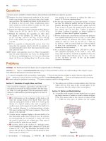
4. O The cutting tool on a lathe is given two displacements,
one of magnitude 4 cm and one of magnitude 3 cm, in
each one of five situations (a) through (e) diagrammed
in Figure Q3.4. Rank these situations according to the
magnitude of the total displacement of the tool, putting
the situation with the greatest resultant magnitude first. If
the total displacement is the same size in two situations,
give those letters equal ranks.

(a)

(b)

D1

(c)

(d)

(e)

Figure Q3.4
D2

S

(a)

(b)
Figure Q3.3

(c)

(d)

5. O Let A represent a velocity vector pointing from the origin into the second quadrant. (a) Is its x component positive, negative, or zero? (b) Is its y component positive,
S
negative, or zero? Let B represent a velocity vector point-


Problems

ing from the origin into the fourth quadrant. (c) Is its x
component positive, negative, or zero? (d) Is its y component positive, negative, or zero? (e) Consider the vector
S
S
A ϩ B. What, if anything, can you conclude about quadrants it must be in or cannot be in? (f) Now consider the
S
S
vector B Ϫ A. What, if anything, can you conclude about
quadrants it must be in or cannot be in?
6. O (i) What is the magnitude of the vector
ˆ 2 m>s? (a) 0 (b) 10 m/s (c) Ϫ10 m/s
110ˆi Ϫ 10k

(d) 10 (e) Ϫ10 (f) 14.1 m/s (g) undefined (ii) What
is the y component of this vector? (Choose from among
the same answers.)
7. O A submarine dives from the water surface at an angle
of 30° below the horizontal, following a straight path 50
m long. How far is the submarine then below the water
surface? (a) 50 m (b) sin 30° (c) cos 30° (d) tan 30°
(e) (50 m)/sin 30° (f) (50 m)/cos 30° (g) (50 m)/
tan 30° (h) (50 m)sin 30° (i) (50 m)cos 30°
(j) (50 m)tan 30° (k) (sin 30°)/50 m (l) (cos 30°)/50 m
(m) (tan 30°)/50 m (n) 30 m (o) 0 (p) none of these
answers
8. O (i) What is the x component of the vector shown in
Figure Q3.8? (a) 1 cm (b) 2 cm (c) 3 cm (d) 4 cm
(e) 6 cm (f) Ϫ1 cm (g) Ϫ2 cm (h) Ϫ3 cm (i) Ϫ4 cm

65

(j) Ϫ6 cm (k) none of these answers (ii) What is the y
component of this vector? (Choose from among the same
answers.)
y, cm
2
Ϫ4 Ϫ2

0

2

x, cm

Ϫ2
Figure Q3.8
S

9. O Vector A lies in the xy plane. (i) Both of its components
will be negative if it lies in which quadrant(s)? Choose all
that apply. (a) the first quadrant (b) the second quadrant (c) the third quadrant (d) the fourth quadrant
(ii) For what orientation(s) will its components have opposite signs? Choose from among the same possibilities.
S
10. If the component of vector A along the direction of vector
S
B is zero, what can you conclude about the two vectors?
11. Can the magnitude of a vector have a negative value?
Explain.
12. Is it possible to add a vector quantity to a scalar quantity?
Explain.

Problems
The Problems from this chapter may be assigned online in WebAssign.
Sign in at www.thomsonedu.com and go to ThomsonNOW to assess your understanding of this chapter’s topics
with additional quizzing and conceptual questions.
1, 2, 3 denotes straightforward, intermediate, challenging; Ⅺ denotes full solution available in Student Solutions Manual/Study
Guide ; ᮡ denotes coached solution with hints available at www.thomsonedu.com; Ⅵ denotes developing symbolic reasoning;
ⅷ denotes asking for qualitative reasoning;
denotes computer useful in solving problem
Section 3.1 Coordinate Systems
1. ᮡ The polar coordinates of a point are r ϭ 5.50 m and
u ϭ 240°. What are the Cartesian coordinates of this point?
2. Two points in a plane have polar coordinates (2.50 m,

30.0°) and (3.80 m, 120.0°). Determine (a) the Cartesian
coordinates of these points and (b) the distance between
them.
3. A fly lands on one wall of a room. The lower left-hand corner of the wall is selected as the origin of a two-dimensional
Cartesian coordinate system. If the fly is located at the
point having coordinates (2.00, 1.00) m, (a) how far is it
from the corner of the room? (b) What is its location in
polar coordinates?
4. The rectangular coordinates of a point are given by (2, y),
and its polar coordinates are (r, 30°). Determine y and r.
5. Let the polar coordinates of the point (x, y) be (r, u).
Determine the polar coordinates for the points (a) (Ϫx, y),
(b) (Ϫ2x, Ϫ2y), and (c) (3x, Ϫ3y).
2 = intermediate;

3 = challenging;

Ⅺ = SSM/SG;

ᮡ

Section 3.2 Vector and Scalar Quantities
Section 3.3 Some Properties of Vectors
6. A plane flies from base camp to lake A, 280 km away in
the direction 20.0° north of east. After dropping off supplies it flies to lake B, which is 190 km at 30.0° west of
north from lake A. Graphically determine the distance
and direction from lake B to the base camp.
7. A surveyor measures the distance across a straight river by
the following method: starting directly across from a tree
on the opposite bank, she walks 100 m along the riverbank to establish a baseline. Then she sights across to the

tree. The angle from her baseline to the tree is 35.0°.
How wide is the river?
S
8. A force F1 of magnitude 6.00 units acts on an object at
the origin in a direction 30.0° above the positive x axis. A
S
second force F2 of magnitude 5.00 units acts on the object
in the direction of the positive y axis. Graphically find the
S
S
magnitude and direction of the resultant force F1 ϩ F2.

= ThomsonNOW;

Ⅵ = symbolic reasoning;

ⅷ = qualitative reasoning


66

Chapter 3

Vectors

ᮡ

A skater glides along a circular path of radius 5.00 m. If
he coasts around one half of the circle, find (a) the magnitude of the displacement vector and (b) how far he
skated. (c) What is the magnitude of the displacement if

he skates all the way around the circle?
10. Arbitrarily define the “instantaneous vector height” of a
person as the displacement vector from the point halfway
between his or her feet to the top of the head. Make an
order-of-magnitude estimate of the total vector height of
all the people in a city of population 100 000 (a) at
10 o’clock on a Tuesday morning and (b) at 5 o’clock on
a Saturday morning. Explain your reasoning.
S
S
11. ᮡ Each of the displacement vectors A and B shown in
Figure P3.11 has a magnitude of 3.00 m. Graphically find
S
S
S
S
S
S
S
S
(a) A ϩ B, (b) A Ϫ B, (c) B Ϫ A, and (d) A Ϫ 2B. Report
all angles counterclockwise from the positive x axis.
9.

18.

19.

20.

21.

y
B

22.

3.00 m

A

0m
3.0
30.0Њ

x

O
Figure P3.11

23.
Problems 11 and 32.
S

12. ⅷ Three displacementsS are A ϭ 200 m due south, B ϭ
250 m due west, and C ϭ 150 m at 30.0° east of north.
Construct a separate diagram for each Sof the
following
S
S

S
possible
ways
of
adding
these
vectors:
R
ϭ
A
ϩ
B ϩ C;
1
S
S
S
S
S
S
S
S
R2 ϭ B ϩ C ϩ A; R3 ϭ C ϩ B ϩ A. Explain what you can
conclude from comparing the diagrams.
13. A roller-coaster car moves 200 ft horizontally and then
rises 135 ft at an angle of 30.0° above the horizontal. It
next travels 135 ft at an angle of 40.0° downward. What is
its displacement from its starting point? Use graphical
techniques.
14. ⅷ A shopper pushing a cart through a store moves 40.0 m
down one aisle, then makes a 90.0° turn and moves 15.0 m.

He then makes another 90.0° turn and moves 20.0 m.
(a) How far is the shopper away from his original position? (b) What angle does his total displacement make
with his original direction? Notice that we have not specified whether the shopper turned right or left. Explain
how many answers are possible for parts (a) and (b) and
give the possible answers.
S

Section 3.4 Components of a Vector and Unit Vectors
15. ᮡ A vector has an x component of Ϫ25.0 units and a y
component of 40.0 units. Find the magnitude and direction of this vector.
16. A person walks 25.0° north of east for 3.10 km. How far
would she have to walk due north and due east to arrive
at the same location?
17. ⅷ A minivan travels straight north in the right lane of a
divided highway at 28.0 m/s. A camper passes the minivan and then changes from the left into the right lane. As
it does so, the camper’s path on the road is a straight displacement at 8.50° east of north. To avoid cutting off the
minivan, the north–south distance between the camper’s
2 = intermediate;

3 = challenging;

Ⅺ = SSM/SG;

ᮡ

24.

25.

26.

rear bumper and the minivan’s front bumper should not
decrease. Can the camper be driven to satisfy this requirement? Explain your answer.
A girl delivering newspapers covers her route by traveling
3.00 blocks west, 4.00 blocks north, and then 6.00 blocks
east. (a) What is her resultant displacement? (b) What is
the total distance she travels?
Obtain expressions in component form for the position
vectors having the following polar coordinates: (a) 12.8 m,
150° (b) 3.30 cm, 60.0° (c) 22.0 in., 215°
A displacement vector lying in the xy plane has a magnitude of 50.0 m and is directed at an angle of 120° to the
positive x axis. What are the rectangular components of
this vector?
While exploring a cave, a spelunker starts at the entrance
and moves the following distances. She goes 75.0 m
north, 250 m east, 125 m at an angle 30.0° north of east,
and 150 m south. Find her resultant displacement from
the cave entrance.
A map suggests that Atlanta is 730 miles in a direction of
5.00° north of east from Dallas. The same map shows that
Chicago is 560 miles in a direction of 21.0° west of north
from Atlanta. Modeling the Earth as flat, use this information to find the displacement from Dallas to Chicago.
A man pushing a mop across a floor causes it to undergo
two displacements. The first has a magnitude of 150 cm
and makes an angle of 120° with the positive x axis. The
resultant displacement has a magnitude of 140 cm and is
directed at an angle of 35.0° to the positive x axis. Find
the magnitude and direction of the second displacement.
S
S

Given the vectors A ϭ 2.00ˆi ϩ 6.00ˆj and B ϭ 3.00ˆi Ϫ
S
S
S
2.00ˆj , (a) draw the vector sum C ϭ A ϩ B and the vector
S
S
S
S
S
difference D ϭ A Ϫ B. (b) Calculate C and D, first in
terms of unit vectors and then in terms of polar coordinates, with angles measured with respect to the ϩx axis.
S
S
Consider the two vectors A ϭ 3ˆi Ϫ 2jˆ and B ϭ Ϫ ˆi Ϫ 4ˆj .
S
S
S
S
S
S
S
S
Calculate (a) A ϩ B, (b) A Ϫ B, (c) 0 A ϩ B 0 , (d) 0 A Ϫ B 0 ,
S
S
S
S
and (e) the directions of A ϩ B and A Ϫ B.
A snow-covered ski slope makes an angle of 35.0° with the

horizontal. When a ski jumper plummets onto the hill, a
parcel of splashed snow projects to a maximum position
of 5.00 m at 20.0° from the vertical in the uphill direction
as shown in Figure P3.26. Find the components of its
maximum position (a) parallel to the surface and (b) perpendicular to the surface.

20.0°

35.0°

Figure P3.26

27. A particle undergoes the following consecutive displacements: 3.50 m south, 8.20 m northeast, and 15.0 m west.
What is the resultant displacement?

= ThomsonNOW;

Ⅵ = symbolic reasoning;

ⅷ = qualitative reasoning


Problems

28. In a game of American football, a quarterback takes the
ball from the line of scrimmage, runs backward a distance
of 10.0 yards, and then runs sideways parallel to the line
of scrimmage for 15.0 yards. At this point, he throws a forward pass 50.0 yards straight downfield perpendicular to
the line of scrimmage. What is the magnitude of the football’s resultant displacement?
29. A novice golfer on the green takes three strokes to sink

the ball. The successive displacements of the ball are 4.00 m
to the north, 2.00 m northeast, and 1.00 m at 30.0° west
of south. Starting at the same initial point, an expert
golfer could make the hole in what single displacement?
S
30. Vector A has x and y components of Ϫ8.70 cm and 15.0 cm,
S
respectively; vector B has x and y components of 13.2 cm
S
S
S
and Ϫ6.60 cm, respectively. If A Ϫ B ϩ 3C ϭ 0, what are
S
the components of C?
31. The helicopter view in Figure P3.31 shows two people
pulling on a stubborn mule. Find (a) the single force that
is equivalent to the two forces shown and (b) the force
that a third person would have to exert on the mule to
make the resultant force equal to zero. The forces are
measured in units of newtons (symbolized N).

Figure P3.36

37.

38.
y

F1 ϭ
120 N

F2 ϭ
80.0 N
75.0Њ

60.0Њ

x

39.

Figure P3.31
S

S

32. Use the component method to add the vectors A and B
S
S
shown in Figure P3.11. Express the resultant A ϩ B in
unit–vector notation.
S
33. Vector B has x, y, and z components of 4.00, 6.00, and
S
3.00 units, respectively. Calculate the magnitude of B and
S
the angles B makes with the coordinate axes.
S
34. Consider
the three displacement

vectors A ϭ 13ˆi Ϫ 3ˆj 2 m,
S
S
B ϭ 1 ˆi Ϫ 4ˆj 2 m, and C ϭ 1Ϫ2ˆi ϩ 5ˆj 2 m. Use the component method to determine (a) the magnitude and
S
S
S
S
direction of the vector D ϭ A ϩ B ϩ C and (b) the magS
S
S
S
nitude and direction of E ϭ ϪA Ϫ B ϩ C.
S
ˆ2 m
35. GivenS the displacement vectors A ϭ 13ˆi Ϫ 4ˆj ϩ 4k
ˆ2 m, find the magnitudes of the
and B ϭ 12ˆi ϩ 3ˆj Ϫ 7k
S
S
S
S
S
S
vectors (a) C ϭ A ϩ B and (b) D ϭ 2A Ϫ B, also expressing each in terms of its rectangular components.
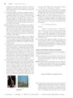
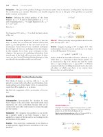
36. In an assembly operation illustrated in Figure P3.36, a
robot moves an object first straight upward and then also
to the east, around an arc forming one quarter of a circle
of radius 4.80 cm that lies in an east–west vertical plane.
The robot then moves the object upward and to the

north, through one-quarter of a circle of radius 3.70 cm
that lies in a north–south vertical plane. Find (a) the mag2 = intermediate;

3 = challenging;

Ⅺ = SSM/SG;

ᮡ

67

40.

41.

42.

43.

nitude of the total displacement of the object and (b) the
angle the total displacement makes with the vertical.
S
The vector A has x, y, and z components of 8.00, 12.0, and
–4.00 units, respectively. (a) Write a vector expression for
S
A in unit–vector notation. (b) Obtain a unit–vector expresS
S
sion for a vector B one-fourth the length of A pointing in
S
the same direction as A. (c) Obtain a unit–vector expresS

S
sion for a vector C three times the length of A pointing in
S
the direction opposite the direction of A.
You are standing on the ground at the origin of a coordinate system. An airplane flies over you with constant
velocity parallel to the x axis and at a fixed height of 7.60 ϫ
103 m. At time t ϭ 0 the airplane is directly above you
so
S
that the vector leading from you to it is P0 ϭ
17.60 ϫ 103 m 2 ˆj . At t ϭ 30.0 sSthe position vector leading from you to the airplane is P30 ϭ 18.04 ϫ 103 m 2 ˆi ϩ
17.60 ϫ 103 m 2 ˆj . Determine the magnitude and orientation of the airplane’s position vector at t ϭ 45.0 s.
A radar station locates a sinking ship at range 17.3 km
and bearing 136° clockwise from north. From the same
station, a rescue plane is at horizontal range 19.6 km,
153° clockwise from north, with elevation 2.20 km.
(a) Write the position vector for the ship relative to the
plane, letting ˆi represent east, ˆj north, and ˆ
k up. (b) How
far apart are the plane and ship?
S
(a) Vector E has magnitude 17.0 cm and is directed 27.0°
counterclockwise from the ϩx axis. Express it in unit–vector
S
notation. (b) Vector F has magnitude 17.0 cm and is
directed 27.0° counterclockwise from the ϩy axis. Express
S
it in unit–vector notation. (c) Vector G has magnitude
17.0 cm and is directed 27.0° clockwise from the Ϫy axis.
Express it in unit–vector notation.

S
Vector A has a negative x component 3.00 units in
length and a positive y component 2.00 units in length.
S
(a) Determine an expression for A in unit–vector notaS
tion. (b) Determine the magnitude and direction of A.
S
S
(c) What vector B when added to A gives a resultant vector with no x component and a negative y component
4.00 units in length?
As it passes over Grand Bahama Island, the eye of a hurricane is moving in a direction 60.0° north of west with a
speed of 41.0 km/h. Three hours later the course of the
hurricane suddenly shifts due north, and its speed slows
to 25.0 km/h. How far from Grand Bahama is the eye
4.50 h after it passes over the island?
ᮡ Three displacement vectors of a croquet ball are shown
S
S
in Figure P3.43, where 0 A 0 ϭ 20.0 units, 0 B 0 ϭ 40.0 units,
S
and 0 C 0 ϭ 30.0 units. Find (a) the resultant in unit–vector

= ThomsonNOW;

Ⅵ = symbolic reasoning;

ⅷ = qualitative reasoning


68

Chapter 3

Vectors

notation and (b) the magnitude and direction of the
resultant displacement.
y

B
A

47.

45.0Њ

O

x

45.0Њ
C

48.
Figure P3.43

44. ⅷ (a) Taking A ϭS 16.00ˆi Ϫ 8.00ˆj 2 units, B ϭ 1Ϫ8.00ˆi ϩ
ˆi ϩ 19.0ˆj 2 units, determine a
3.00ˆj 2 units, and C ϭ
126.0

S
S
S
and b such that a A ϩ b B ϩ C ϭ 0. (b) A student has
learned that a single equation cannot be solved to determine values for more than one unknown in it. How would
you explain to him that both a and b can be determined
from the single equation used in part (a)?
45. ⅷ Are we there yet? In Figure P3.45, the line segment represents a path from the point with position vector
15ˆi ϩ 3ˆj 2 m to the point with location 116ˆi ϩ 12ˆj 2 m.
Point A is along this path, a fraction f of the way to the
destination. (a) Find the position vector of point A in
terms of f. (b) Evaluate the expression from part (a) in
the case f ϭ 0. Explain whether the result is reasonable.
(c) Evaluate the expression for f ϭ 1. Explain whether the
result is reasonable.
S

S

y

49.

50.

map of the successive displacements. (b) What total distance did she travel? (c) Compute the magnitude and
direction of her total displacement. The logical structure
of this problem and of several problems in later chapters
was suggested by Alan Van Heuvelen and David Maloney,
American Journal of Physics 67(3) 252–256, March 1999.

S
S
Two vectors A and B have precisely equal magnitudes. For
S
S
the magnitude of A ϩ B to be 100 times larger than the
S
S
magnitude of A Ϫ B, what must be the angle between
them?
S
S
Two vectors A and B have precisely equal magnitudes. For
S
S
the magnitude of A ϩ B to be larger than the magnitude
S
S
of A Ϫ B by the factor n, what must be the angle between
them?
An air-traffic controller observes two aircraft on his radar
screen. The first is at altitude 800 m, horizontal distance
19.2 km, and 25.0° south of west. The second is at altitude
1 100 m, horizontal distance 17.6 km, and 20.0° south of
west. What is the distance between the two aircraft? (Place
the x axis west, the y axis south, and the z axis vertical.)
The biggest stuffed animal in the world is a snake 420 m
long, constructed by Norwegian children. Suppose the
snake is laid out in a park as shown in Figure P3.50, forming two straight sides of a 105° angle, with one side 240 m
long. Olaf and Inge run a race they invent. Inge runs

directly from the tail of the snake to its head, and Olaf
starts from the same place at the same moment but runs
along the snake. If both children run steadily at 12.0 km/h,
Inge reaches the head of the snake how much earlier
than Olaf?

(16, 12)

A
(5, 3)
O

x

Figure P3.45 Point A is a fraction f of the distance from the initial point (5, 3) to the final point (16, 12).

Additional Problems
46. On December 1, 1955, Rosa Parks (1913–2005), an icon of
the early civil rights movement, stayed seated in her bus
seat when a white man demanded it. Police in Montgomery, Alabama, arrested her. On December 5, blacks
began refusing to use all city buses. Under the leadership
of the Montgomery Improvement Association, an efficient
system of alternative transportation sprang up immediately, providing blacks with approximately 35 000 essential
trips per day through volunteers, private taxis, carpooling,
and ride sharing. The buses remained empty until they
were integrated under court order on December 21, 1956.
In picking up her riders, suppose a driver in downtown
Montgomery traverses four successive displacements represented by the expression

1Ϫ6.30b2 ˆi Ϫ 14.00b cos 40° 2 ˆi Ϫ 14.00b sin 40°2 ˆj

ϩ 13.00b cos 50°2 ˆi Ϫ 13.00b sin 50°2 ˆj Ϫ 15.00b2 ˆj

Here b represents one city block, a convenient unit of distance of uniform size; ˆi is east; and ˆj is north. (a) Draw a
2 = intermediate;

3 = challenging;

Ⅺ = SSM/SG;

ᮡ

Figure P3.50

51. A ferryboat transports tourists among three islands. It sails
from the first island to the second island, 4.76 km away, in
a direction 37.0° north of east. It then sails from the second island to the third island in a direction 69.0° west of
north. Finally, it returns to the first island, sailing in a
direction 28.0° east of south. Calculate the distance
between (a) the second and third islands and (b) the first
and third islands.
S
ˆ. Find (a) the magni52. A vector is given by R ϭ 2ˆi ϩ ˆj ϩ 3k
tudes of the x, y, and z components, (b) the magnitude of
S
S
R, and (c) the angles between R and the x, y, and z axes.
53. A jet airliner, moving initially at 300 mi/h to the east,
suddenly enters a region where the wind is blowing at
100 mi/h toward the direction 30.0° north of east. What

are the new speed and direction of the aircraft relative to
the ground?
S
54. ⅷ Let A ϭ 60.0 cm at 270° measured from the horizontal.
S
Let B ϭ 80.0 cm at some angle u. (a) Find the magnitude
S
S
of A ϩ B as a function of u. (b) From the answer to part
S
S
(a), for what value of u does 0 A ϩ B 0 take on its maximum

= ThomsonNOW;

Ⅵ = symbolic reasoning;

ⅷ = qualitative reasoning


Problems

value? What is this maximum value? (c) From the answer
S
S
to part (a), for what value of u does 0 A ϩ B 0 take on its
minimum value? What is this minimum value? (d) Without reference to the answer to part (a), argue that the
answers to each of parts (b) and (c) do or do not make
sense.
55. After a ball rolls off the edge of a horizontal table at time

t ϭ 0, its velocity as a function of time is given by
v ϭ 1.2ˆi m>s Ϫ 9.8tˆj m>s2

S

The ball’s displacement away from the edge of the table,
during the time interval of 0.380 s during which it is in
flight, is given by
0.380 s

¢r ϭ
S

Ύ v dt
S

0

To perform the integral, you can use the calculus theorem

Ύ 1A ϩ Bf 1x 2 2 dx ϭ Ύ A dx ϩ B Ύ f 1x 2 dx
You can think of the units and unit vectors as constants,
represented by A and B. Do the integration to calculate
the displacement of the ball.
56. ⅷ Find the sum of these four vector forces: 12.0 N to the
right at 35.0° above the horizontal, 31.0 N to the left at
55.0° above the horizontal, 8.40 N to the left at 35.0°
below the horizontal, and 24.0 N to the right at 55.0°
below the horizontal. Follow these steps. Guided by a
sketch of this situation, explain how you can simplify the

calculations by making a particular choice for the directions of the x and y axes. What is your choice? Then add
the vectors by the component method.
57. A person going for a walk follows the path shown in Figure P3.57. The total trip consists of four straight-line
paths. At the end of the walk, what is the person’s resultant displacement measured from the starting point?
y
Start 100 m

x

300 m

End
200 m
60.0Њ

30.0Њ
150 m

Figure P3.57

58. ⅷ The instantaneous position of an object is specified by
its position vector Sr leading from a fixed origin to the
location of the object, modeled as a particle. Suppose for
a certain object the position vector is a function of time,
S
given by r ϭ 4ˆi ϩ 3ˆj Ϫ 2t ˆ
k , where r is in meters and t is
in seconds. Evaluate drS>dt. What does it represent about
the object?
59. ⅷ Long John Silver, a pirate, has buried his treasure on

an island with five trees, located at the points (30.0 m,
Ϫ20.0 m), (60.0 m, 80.0 m), (Ϫ10.0 m, Ϫ10.0 m), (40.0 m,
Ϫ30.0 m), and (Ϫ70.0 m, 60.0 m), all measured relative
2 = intermediate;

3 = challenging;

Ⅺ = SSM/SG;

ᮡ

69

to some origin as shown in Figure P3.59. His ship’s log
instructs you to start at tree A and move toward tree B,
but to cover only one-half the distance between A and B.
Then move toward tree C, covering one-third the distance
between your current location and C. Next move toward
tree D, covering one-fourth the distance between where you
are and D. Finally, move toward tree E, covering one-fifth
the distance between you and E, stop, and dig. (a) Assume
you have correctly determined the order in which the
pirate labeled the trees as A, B, C, D, and E as shown in
the figure. What are the coordinates of the point where
his treasure is buried? (b) What If? What if you do not
really know the way the pirate labeled the trees? What
would happen to the answer if you rearranged the order
of the trees, for instance to B(30 m, Ϫ20 m), A(60 m,
80 m), E(Ϫ10 m, –10 m), C(40 m, Ϫ30 m), and
D(Ϫ70 m, 60 m)? State reasoning to show the answer

does not depend on the order in which the trees are
labeled.

B
E

y

x
C
A
D
Figure P3.59

60. ⅷ Consider a game in which N children position themselves at equal distances around the circumference of a
circle. At the center of the circle is a rubber tire. Each
child holds a rope attached to the tire and, at a signal,
pulls on his or her rope. All children exert forces of the
same magnitude F. In the case N ϭ 2, it is easy to see that
the net force on the tire will be zero because the two
oppositely directed force vectors add to zero. Similarly, if
N ϭ 4, 6, or any even integer, the resultant force on the
tire must be zero because the forces exerted by each pair
of oppositely positioned children will cancel. When an
odd number of children are around the circle, it is not as
obvious whether the total force on the central tire will be
zero. (a) Calculate the net force on the tire in the case
N ϭ 3 by adding the components of the three force vectors. Choose the x axis to lie along one of the ropes.
(b) What If? State reasoning that will determine the net
force for the general case where N is any integer, odd or

even, greater than one. Proceed as follows. Assume the
total force is not zero. Then it must point in some particular direction. Let every child move one position clockwise. Give a reason that the total force must then have a
direction turned clockwise by 360°/N. Argue that the
total force must nevertheless be the same as before.
Explain what the contradiction proves about the magnitude
of the force. This problem illustrates a widely useful technique of proving a result “by symmetry,” by using a bit
of the mathematics of group theory. The particular situation is actually encountered in physics and chemistry

= ThomsonNOW;

Ⅵ = symbolic reasoning;

ⅷ = qualitative reasoning


70

Chapter 3

Vectors

when an array of electric charges (ions) exerts electric
forces on an atom at a central position in a molecule or
in a crystal.
S
S
61. Vectors
A and
B have equal magnitudes of 5.00. The sum
S

S
of A and B is the vector 6.00ˆj . Determine the angle
S
S
between A and B.
62. A rectangular parallelepiped has dimensions a, b, and c as
shown in Figure P3.62. (a)
Obtain a vector expression for
S
the face diagonal vector R1. What is the magnitude of this
vector? (b)SObtain a vectorSexpression Sfor the body diagonal vector R2. Notice that R1, c ˆ
k , and R2 make a right triS
angle. Prove that the magnitude of R2 is 1 a 2 ϩ b 2 ϩ c 2.

z
a

b

O
x

R2

c

R1
y
Figure P3.62

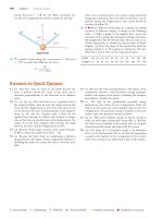
Answers to Quick Quizzes
3.1 Scalars: (a), (d), (e). None of these quantities has a direction. Vectors: (b), (c). For these quantities, the direction
is necessary to specify the quantity completely.
3.2 (c). The resultant has its maximum magnitude A ϩ B ϭ
S
12 ϩ 8 ϭ 20 units when vector A is oriented in the same
S
direction as vector B. The resultant vector has its miniS
mum magnitude A Ϫ B ϭ 12 Ϫ 8 ϭ 4 units when vector A
S
is oriented in the direction opposite vector B.
3.3 (b) and (c). To add to zero, the vectors must point in
opposite directions and have the same magnitude.

2 = intermediate;

3 = challenging;

Ⅺ = SSM/SG;

ᮡ

3.4 (b). From the Pythagorean theorem, the magnitude of a
vector is always larger than the absolute value of each
component, unless there is only one nonzero component,
in which case the magnitude of the vector is equal to the
absolute value of that component.
S
3.5 (c). The magnitude of C is 5 units, the same as the z component. Answer (b) is not correct because the magnitude
of any vector is always a positive number, whereas the y

S
component of B is negative.

= ThomsonNOW;

Ⅵ = symbolic reasoning;

ⅷ = qualitative reasoning


4.1

The Position, Velocity, and Acceleration Vectors

4.2

Two-Dimensional Motion with Constant Acceleration

4.3

Projectile Motion

4.4

The Particle in Uniform Circular Motion

4.5

Tangential and Radial Acceleration

4.6

Relative Velocity and Relative Acceleration

Lava spews from a volcanic eruption. Notice the parabolic paths of embers
projected into the air. All projectiles follow a parabolic path in the absence
of air resistance. (© Arndt/Premium Stock/PictureQuest)

4

Motion in Two Dimensions

In this chapter, we explore the kinematics of a particle moving in two dimensions.
Knowing the basics of two-dimensional motion will allow us—in future chapters—
to examine a variety of motions ranging from the motion of satellites in orbit to
the motion of electrons in a uniform electric field. We begin by studying in greater
detail the vector nature of position, velocity, and acceleration. We then treat projectile motion and uniform circular motion as special cases of motion in two
dimensions. We also discuss the concept of relative motion, which shows why
observers in different frames of reference may measure different positions and
velocities for a given particle.

4.1

The Position, Velocity, and
Acceleration Vectors

In Chapter 2, we found that the motion of a particle along a straight line is completely known if its position is known as a function of time. Let us now extend this
idea to two-dimensional motion of a particle in the xy plane. We begin by describing
S
the position of the particle by its position vector r , drawn from the origin of some

coordinate system to the location of the particle in the xy plane, as in Figure 4.1
S
(page 72). At time ti, the particle is at point Ꭽ, described by position vector r i. At
S
some later time tf , it is at point Ꭾ, described by position vector r f . The path from
71


72

Chapter 4

Motion in Two Dimensions

Ꭽ to Ꭾ is not necessarily a straight line. As the particle moves from Ꭽ to Ꭾ in the
S
S
time interval ⌬t ϭ tf Ϫ ti, its position vector changes from r i to r f . As we learned in
Chapter 2, displacement is a vector, and the displacement of the particle is the difference between its final position and its initial position. We now define the disS
placement vector ¢r for a particle such as the one in Figure 4.1 as being the difference between its final position vector and its initial position vector:
Displacement vector

¢r ϵ r f Ϫ r i
S

ᮣ

S

S

(4.1)

S

The direction of ¢r is indicated in Figure 4.1. As we see from the figure, the magS
nitude of ¢r is less than the distance traveled along the curved path followed by
the particle.
As we saw in Chapter 2, it is often useful to quantify motion by looking at the
ratio of a displacement divided by the time interval during which that displacement occurs, which gives the rate of change of position. Two-dimensional (or
three-dimensional) kinematics is similar to one-dimensional kinematics, but we
must now use full vector notation rather than positive and negative signs to indicate the direction of motion.
S
We define the average velocity vavg of a particle during the time interval ⌬t as
the displacement of the particle divided by the time interval:
S

Average velocity

ᮣ

y

Ꭽ ti

⌬r

ri
rf
O

Ꭾ tf
Path of
particle
x

Figure 4.1 A particle moving in the
xy plane is located with the position
S
vector r drawn from the origin
to the particle. The displacement of
the particle as it moves from Ꭽ to Ꭾ
in the time interval ⌬t ϭ tf Ϫ ti is
S
S
S
equal to the vector ¢ r ϭ r f Ϫ r i.

vavg ϵ

S

¢r
¢t

(4.2)

Multiplying or dividing a vector quantity by a positive scalar quantity such as ⌬t
changes only the magnitude of the vector, not its direction. Because displacement
is a vector quantity and the time interval is a positive scalar quantity, we conclude

S
that the average velocity is a vector quantity directed along ¢r .
The average velocity between points is independent of the path taken. That is
because average velocity is proportional to displacement, which depends only on
the initial and final position vectors and not on the path taken. As with onedimensional motion, we conclude that if a particle starts its motion at some point
and returns to this point via any path, its average velocity is zero for this trip
because its displacement is zero. Consider again our basketball players on the court
in Figure 2.2 (page 21). We previously considered only their one-dimensional
motion back and forth between the baskets. In reality, however, they move over a
two-dimensional surface, running back and forth between the baskets as well as
left and right across the width of the court. Starting from one basket, a given
player may follow a very complicated two-dimensional path. Upon returning to the
original basket, however, a player’s average velocity is zero because the player’s displacement for the whole trip is zero.
Consider again the motion of a particle between two points in the xy plane as
shown in Figure 4.2. As the time interval over which we observe the motion
y

Ꭽ

Direction of v at Ꭽ

⌬r1 ⌬r2 ⌬r3
Figure 4.2 As a particle moves between two points, its
average velocity is in the direction of the displacement vecS
tor ¢ r . As the end point of the path is moved from Ꭾ to
Ꭾ¿ to Ꭾ– , the respective displacements and corresponding time intervals become smaller and smaller. In the
limit that the end point approaches Ꭽ, ⌬t approaches zero
S
and the direction of ¢ r approaches that of the line tangent to the curve at Ꭽ. By definition, the instantaneous
velocity at Ꭽ is directed along this tangent line.

ᎮЉ
ᎮЈ
Ꭾ
O

x


Section 4.1

The Position, Velocity, and Acceleration Vectors

73

becomes smaller and smaller—that is, as Ꭾ is moved to Ꭾ¿ and then to Ꭾ– , and
so on—the direction of the displacement approaches that of the line tangent to
S
the path at Ꭽ. The instantaneous velocity v is defined as the limit of the average
S
velocity ¢ r >¢t as ⌬t approaches zero:
S

v ϵ lim

S

¢tS0

S

¢r
dr
ϭ
¢t
dt

(4.3)

ᮤ

Instantaneous velocity

ᮤ

Average acceleration

ᮤ

Instantaneous acceleration

That is, the instantaneous velocity equals the derivative of the position vector with
respect to time. The direction of the instantaneous velocity vector at any point in a
particle’s path is along a line tangent to the path at that point and in the direction
of motion.
S
The magnitude of the instantaneous velocity vector v ϭ 0 v 0 of a particle is called
the speed of the particle, which is a scalar quantity.
As a particle moves from one point to another along some path, its instantaS
S

neous velocity vector changes from vi at time ti to vf at time tf. Knowing the velocity
at these points allows us to determine the average acceleration of the particle. The
S
average acceleration aavg of a particle is defined as the change in its instantaneous
S
velocity vector ¢v divided by the time interval ⌬t during which that change occurs:
vf Ϫ vi

S

aavg ϵ

S

S

tf Ϫ ti

S

ϭ

¢v
¢t

(4.4)

Because aavg is the ratio of a vector quantity ¢v and a positive scalar quantity ⌬t, we
S
conclude that average acceleration is a vector quantity directed along ¢v. As indiS

S
cated in Figure 4.3, the direction of ¢v is found by adding the vector Ϫvi (the
S
S
S
S
S
negative of vi) to the vector vf because, by definition, ¢v ϭ vf Ϫ vi.
When the average acceleration of a particle changes during different time intervals, it is useful to define its instantaneous acceleration. The instantaneous accelerS
S
ation a is defined as the limiting value of the ratio ¢v>¢t as ⌬t approaches zero:
S

S

S

a ϵ lim

S

¢tS0

S

¢v
dv
ϭ
dt
¢t

(4.5)

In other words, the instantaneous acceleration equals the derivative of the velocity
vector with respect to time.
Various changes can occur when a particle accelerates. First, the magnitude of the
velocity vector (the speed) may change with time as in straight-line (one-dimensional)
motion. Second, the direction of the velocity vector may change with time even if
its magnitude (speed) remains constant as in two-dimensional motion along a
curved path. Finally, both the magnitude and the direction of the velocity vector
may change simultaneously.

y

⌬v

Ꭽ

vf

vi
–vi

Ꭾ
vf

ri
rf

O

or

vi
⌬v

vf

x

Figure 4.3 A particle moves from position Ꭽ to position Ꭾ. Its velocity vector changes from vi to vf .
S
The vector diagrams at the upper right show two ways of determining the vector ¢v from the initial and final velocities.
S

S

PITFALL PREVENTION 4.1
Vector Addition
Although the vector addition discussed in Chapter 3 involves displacement vectors, vector addition can be
applied to any type of vector quantity. Figure 4.3, for example, shows
the addition of velocity vectors using
the graphical approach.


74

Chapter 4

Motion in Two Dimensions

Quick Quiz 4.1 Consider the following controls in an automobile: gas pedal,
brake, steering wheel. What are the controls in this list that cause an acceleration
of the car? (a) all three controls (b) the gas pedal and the brake (c) only the
brake (d) only the gas pedal

4.2

Two-Dimensional Motion with
Constant Acceleration

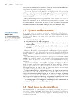
In Section 2.5, we investigated one-dimensional motion of a particle under constant acceleration. Let us now consider two-dimensional motion during which the
acceleration of a particle remains constant in both magnitude and direction. As we
shall see, this approach is useful for analyzing some common types of motion.
Before embarking on this investigation, we need to emphasize an important
point regarding two-dimensional motion. Imagine an air hockey puck moving in a
straight line along a perfectly level, friction-free surface of an air hockey table. Figure 4.4a shows a motion diagram from an overhead point of view of this puck.
Recall that in Section 2.4 we related the acceleration of an object to a force on the
object. Because there are no forces on the puck in the horizontal plane, it moves
with constant velocity in the x direction. Now suppose you blow a puff of air on
the puck as it passes your position, with the force from your puff of air exactly in
the y direction. Because the force from this puff of air has no component in the x
direction, it causes no acceleration in the x direction. It only causes a momentary
acceleration in the y direction, causing the puck to have a constant y component
of velocity once the force from the puff of air is removed. After your puff of air on
the puck, its velocity component in the x direction is unchanged, as shown in Figure 4.4b. The generalization of this simple experiment is that motion in two
dimensions can be modeled as two independent motions in each of the two perpendicular directions associated with the x and y axes. That is, any influence in the y
direction does not affect the motion in the x direction and vice versa.
The position vector for a particle moving in the xy plane can be written
r ϭ xˆi ϩ yˆj

S

(4.6)

where x, y, and r change with time as the particle moves while the unit vectors ˆi
and ˆj remain constant. If the position vector is known, the velocity of the particle
can be obtained from Equations 4.3 and 4.6, which give
S

vϭ

S

S
dy
dr
dx
ϭ ˆi ϩ ˆj ϭ vxˆi ϩ vyˆj
dt
dt
dt

(4.7)

y
x
(a)

y

x
(b)
Figure 4.4 (a) A puck moves across a horizontal air hockey table at constant velocity in the x direction.
(b) After a puff of air in the y direction is applied to the puck, the puck has gained a y component of
velocity, but the x component is unaffected by the force in the perpendicular direction. Notice that the
horizontal red vectors, representing the x component of the velocity, are the same length in both parts
of the figure, which demonstrates that motion in two dimensions can be modeled as two independent
motions in perpendicular directions.


Section 4.2

Two-Dimensional Motion with Constant Acceleration

S

Because the acceleration a of the particle is assumed constant in this discussion,
its components ax and ay also are constants. Therefore, we can model the particle
as a particle under constant acceleration independently in each of the two directions and apply the equations of kinematics separately to the x and y components of
the velocity vector. Substituting, from Equation 2.13, vxf ϭ vxi ϩ axt and vyf ϭ vyi ϩ
ayt into Equation 4.7 to determine the final velocity at any time t, we obtain
vf ϭ 1vxi ϩ axt2 ˆi ϩ 1vyi ϩ ayt2 ˆj ϭ 1vxiˆi ϩ vyiˆj 2 ϩ 1axˆi ϩ ayˆj 2t

S

v f ϭ v i ϩ at

S

S

S

(4.8)

ᮤ

Velocity vector as a
function of time

ᮤ

Position vector as a
function of time

This result states that the velocity of a particle at some time t equals the vector sum
S
S
of its initial velocity vi at time t ϭ 0 and the additional velocity at acquired at time
t as a result of constant acceleration. Equation 4.8 is the vector version of Equation
2.13.
Similarly, from Equation 2.16 we know that the x and y coordinates of a particle
moving with constant acceleration are
x f ϭ x i ϩ v xit ϩ 12a xt 2

y f ϭ y i ϩ v yit ϩ 12a yt 2

Substituting these expressions into Equation 4.6 (and labeling the final position
S
vector r f) gives

r f ϭ 1x i ϩ v xit ϩ 12a xt 2 2 ˆi ϩ 1y i ϩ v yit ϩ 12a yt 2 2 ˆj

S

ϭ 1x iˆi ϩ y iˆj 2 ϩ 1v xiˆi ϩ v yiˆj 2t ϩ 12 1a xˆi ϩ a yˆj 2t 2
(4.9)

r f ϭ r i ϩ vit ϩ 12 at 2

S

S

S

S

which is the vector version of Equation 2.16. Equation 4.9 tells us that the position
S
S
vector r f of a particle is the vector sum of the original position r i, a displacement
S
S
vit arising from the initial velocity of the particle and a displacement 21 at 2 resulting
from the constant acceleration of the particle.
Graphical representations of Equations 4.8 and 4.9 are shown in Active Figure
4.5. The components of the position and velocity vectors are also illustrated in the
S
figure. Notice from Active Figure 4.5a that vf is generally not along the direction
S

S
of either vi or a because the relationship between these quantities is a vector
S
expression. For the same reason, from Active Figure 4.5b we see that r f is generally
S
S
S
S
not along the direction of vi or a. Finally, notice that vf and r f are generally not in
the same direction.

y

y

ayt

vf

vyf
vyi

1 a t2
2 y

at

vyit

vi

x

yi

ri
x
vxit

xi
vxf

at 2

vit

axt

vxi

(a)

1
2

rf

yf

1 a t2
2 x

xf
(b)

ACTIVE FIGURE 4.5
Vector representations and components of (a) the velocity and (b) the position of a particle moving
S
with a constant acceleration a.
Sign in at www.thomsonedu.com and go to ThomsonNOW to investigate the effect of different initial
positions and velocities on the final position and velocity (for constant acceleration).

75


76

Chapter 4

E XA M P L E 4 . 1

Motion in Two Dimensions

Motion in a Plane

A particle starts from the origin at t ϭ 0 with an initial velocity having an x component of 20 m/s and a y component of
Ϫ15 m/s. The particle moves in the xy plane with an x component of acceleration only, given by ax ϭ 4.0 m/s2.
(A) Determine the total velocity vector at any time.
SOLUTION

y

x

Conceptualize The components of the initial velocity tell
us that the particle starts by moving toward the right and
downward. The x component of velocity starts at 20 m/s
and increases by 4.0 m/s every second. The y component of velocity never changes from its initial value of
Ϫ15 m/s. We sketch a motion diagram of the situation
in Figure 4.6. Because the particle is accelerating in the
ϩx direction, its velocity component in this direction
increases and the path curves as shown in the diagram.
Figure 4.6 (Example 4.1) Motion diagram for the particle.
Notice that the spacing between successive images
increases as time goes on because the speed is increasing. The placement of the acceleration and velocity vectors in
Figure 4.6 helps us further conceptualize the situation.
Categorize Because the initial velocity has components in both the x and y directions, we categorize this problem as one
involving a particle moving in two dimensions. Because the particle only has an x component of acceleration, we model
it as a particle under constant acceleration in the x direction and a particle under constant velocity in the y direction.
Analyze

To begin the mathematical analysis, we set vxi ϭ 20 m/s, vyi ϭ Ϫ15 m/s, ax ϭ 4.0 m/s2, and ay ϭ 0.
vf ϭ vi ϩ at ϭ 1vxi ϩ axt2 ˆi ϩ 1vyi ϩ ayt2 ˆj

Use Equation 4.8 for the velocity vector:

S

Substitute numerical values:

S

S

S

vf ϭ 320 m>s ϩ 14.0 m>s2 2t4 ˆi ϩ 3Ϫ15 m>s ϩ 102 t4 ˆj

(1) vf ϭ 3 120 ϩ 4.0t2 ˆi Ϫ 15ˆj 4 m>s
S

Finalize Notice that the x component of velocity increases in time while the y component remains constant; this
result is consistent with what we predicted.
(B) Calculate the velocity and speed of the particle at t ϭ 5.0 s.
SOLUTION
Analyze
Evaluate the result from Equation (1) at t ϭ 5.0 s:
S

Determine the angle u that vf makes with the x axis at
t ϭ 5.0 s:
Evaluate the speed of the particle as the magnitude
S
of vf :

vf ϭ 3 120 ϩ 4.0 15.02 2 ˆi Ϫ 15ˆj 4 m>s ϭ 140ˆi Ϫ 15ˆj 2 m>s

S

u ϭ tanϪ1 a

vyf

vxf

b ϭ tanϪ1 a

Ϫ15 m>s
40 m>s

b ϭ Ϫ21°

vf ϭ 0 vf 0 ϭ 2vxf2 ϩ vyf 2 ϭ 2 1402 2 ϩ 1Ϫ15 2 2 m>s ϭ 43 m>s
S

Finalize The negative sign for the angle u indicates that the velocity vector is directed at an angle of 21° below the
S
positive x axis. Notice that if we calculate vi from the x and y components of vi, we find that vf Ͼ vi. Is that consistent
with our prediction?
(C) Determine the x and y coordinates of the particle at any time t and its position vector at this time.
SOLUTION
Analyze
Use the components of Equation 4.9 with xi ϭ yi ϭ 0 at
t ϭ 0:

x f ϭ v xit ϩ 12 axt 2 ϭ 120t ϩ 2.0t 2 2 m
yf ϭ v yit ϭ 1Ϫ15t2 m


Section 4.3

r f ϭ xfˆi ϩ yfˆj ϭ 3 120t ϩ 2.0t 2 2 ˆi Ϫ 15tˆj 4 m

Let us now consider a limiting case for very large values of t.
x axis as time grows large. Mathematically, Equation (1)
shows that the y component of the velocity remains constant while the x component grows linearly with t. Therefore, when t is very large, the x component of the velocity will be much larger than the y component, suggesting
that the velocity vector becomes more and more parallel
to the x axis. Both xf and yf continue to grow with time,
although xf grows much faster.

What If? What if we wait a very long time and then
observe the motion of the particle? How would we describe
the motion of the particle for large values of the time?
Answer Looking at Figure 4.6, we see the path of the
particle curving toward the x axis. There is no reason to
assume that this tendency will change, which suggests
that the path will become more and more parallel to the

4.3

PITFALL PREVENTION 4.2
Acceleration at the Highest Point

Projectile Motion

Anyone who has observed a baseball in motion has observed projectile motion.
The ball moves in a curved path and returns to the ground. Projectile motion of
an object is simple to analyze if we make two assumptions: (1) the free-fall acceleration is constant over the range of motion and is directed downward,1 and (2) the
effect of air resistance is negligible.2 With these assumptions, we find that the path
of a projectile, which we call its trajectory, is always a parabola as shown in Active
Figure 4.7. We use these assumptions throughout this chapter.
The expression for the position vector of the projectile as a function of time folS
S

lows directly from Equation 4.9, with a ϭ g:
r f ϭ ri ϩ vit ϩ 12 gt2

S

S

S

S

(4.10)

y

vᎮ

vy

vy ϭ 0 vᎯ

g

Ꭿ

൳

u
vi

Ꭾ

vx i

vxi
u

vy

v൳

vy i
ui

Ꭽ

൴

vx i

vx i

x

ui
vy

v൴

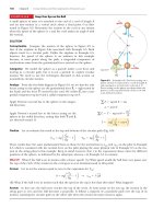
ACTIVE FIGURE 4.7

S

S

The parabolic path of a projectile that leaves the origin with a velocity vi. The velocity vector v changes
with time in both magnitude and direction. This change is the result of acceleration in the negative y
direction. The x component of velocity remains constant in time because there is no acceleration along
the horizontal direction. The y component of velocity is zero at the peak of the path.
Sign in at www.thomsonedu.com and go to ThomsonNOW to change launch angle and initial speed.
You can also observe the changing components of velocity along the trajectory of the projectile.

1

This assumption is reasonable as long as the range of motion is small compared with the radius of the
Earth (6.4 ϫ 106 m). In effect, this assumption is equivalent to assuming that the Earth is flat over the
range of motion considered.

2

77

S

Express the position vector of the particle at any time t:
Finalize

Projectile Motion

This assumption is generally not justified, especially at high velocities. In addition, any spin imparted
to a projectile, such as that applied when a pitcher throws a curve ball, can give rise to some very interesting effects associated with aerodynamic forces, which will be discussed in Chapter 14.

As discussed in Pitfall Prevention
2.8, many people claim that the
acceleration of a projectile at the
topmost point of its trajectory is
zero. This mistake arises from confusion between zero vertical velocity and zero acceleration. If the
projectile were to experience zero
acceleration at the highest point,
its velocity at that point would not
change; rather, the projectile
would move horizontally at constant speed from then on! That
does not happen, however, because
the acceleration is not zero anywhere along the trajectory.


78

Chapter 4

Motion in Two Dimensions

where the initial x and y components of the velocity of the projectile are

The Telegraph Colour Library/Getty Images

vxi ϭ vi cos u i¬¬vyi ϭ vi sin u i

A welder cuts holes through a heavy
metal construction beam with a hot
torch. The sparks generated in the

process follow parabolic paths.

y
1
2

vit

gt 2

(x, y)
rf

x

O
S

Figure 4.8 The position vector r f of
a projectile launched from the origin
whose initial velocity at the origin is
S
S
vi. The vector vit would be the displacement of the projectile if gravity
S
were absent, and the vector 12 gt 2 is its
vertical displacement from a straightline path due to its downward gravitational acceleration.

(4.11)

The expression in Equation 4.10 is plotted in Figure 4.8, for a projectile launched
S
from the origin, so that r i ϭ 0. The final position of a particle can be considered
S
S
to be the superposition of its initial position r i; the term vit, which is its displace1 S 2
ment if no acceleration were present; and the term 2 gt that arises from its acceleration due to gravity. In other words, if there were no gravitational acceleration,
S
the particle would continue to move along a straight path in the direction of vi.
1 S 2
Therefore, the vertical distance 2 gt through which the particle “falls” off the
straight-line path is the same distance that an object dropped from rest would fall
during the same time interval.
In Section 4.2, we stated that two-dimensional motion with constant acceleration
can be analyzed as a combination of two independent motions in the x and y directions, with accelerations ax and ay. Projectile motion can also be handled in this
way, with zero acceleration in the x direction and a constant acceleration in the y
direction, ay ϭ Ϫg. Therefore, when analyzing projectile motion, model it to be the
superposition of two motions: (1) motion of a particle under constant velocity in
the horizontal direction and (2) motion of a particle under constant acceleration
(free fall) in the vertical direction. The horizontal and vertical components of a
projectile’s motion are completely independent of each other and can be handled
separately, with time t as the common variable for both components.

Quick Quiz 4.2 (i) As a projectile thrown upward moves in its parabolic path
(such as in Fig. 4.8), at what point along its path are the velocity and acceleration
vectors for the projectile perpendicular to each other? (a) nowhere (b) the highest point (c) the launch point (ii) From the same choices, at what point are the
velocity and acceleration vectors for the projectile parallel to each other?

Horizontal Range and Maximum Height of a Projectile
Let us assume a projectile is launched from the origin at ti ϭ 0 with a positive vyi

component as shown in Figure 4.9 and returns to the same horizontal level. Two
points are especially interesting to analyze: the peak point Ꭽ, which has Cartesian
coordinates (R/2, h), and the point Ꭾ, which has coordinates (R, 0). The distance
R is called the horizontal range of the projectile, and the distance h is its maximum
height. Let us find h and R mathematically in terms of vi , ui , and g.
We can determine h by noting that at the peak vy Ꭽ ϭ 0. Therefore, we can use
the y component of Equation 4.8 to determine the time t Ꭽ at which the projectile
reaches the peak:
v yf ϭ v yi ϩ a yt
0 ϭ v i sin u i Ϫ gt Ꭽ

y

vi

Ꭽ

tᎭ ϭ

vy Ꭽ ϭ 0

h
ui

Ꭾx

O
R

Figure 4.9 A projectile launched

over a flat surface from the origin at
S
ti ϭ 0 with an initial velocity vi. The
maximum height of the projectile is
h, and the horizontal range is R. At
Ꭽ, the peak of the trajectory, the particle has coordinates (R/2, h).

v i sin u i
g

Substituting this expression for tᎭ into the y component of Equation 4.9 and
replacing y ϭ yᎭ with h, we obtain an expression for h in terms of the magnitude
and direction of the initial velocity vector:
h ϭ 1v i sin u i 2
hϭ

v i2 sin2 u i
2g

v i sin u i 1
v i sin u i 2
Ϫ2ga
b
g
g
(4.12)

The range R is the horizontal position of the projectile at a time that is twice
the time at which it reaches its peak, that is, at time tᎮ ϭ 2tᎭ. Using the x compo-

Section 4.3

Projectile Motion

79

y (m)

150

vi ϭ 50 m/s
75Њ

100

60Њ
45Њ

50

30Њ
15Њ
50

100

150

200

250

x (m)

ACTIVE FIGURE 4.10
A projectile launched over a flat surface from the origin with an initial speed of 50 m/s at various angles of
projection. Notice that complementary values of ui result in the same value of R (range of the projectile).
Sign in at www.thomsonedu.com and go to ThomsonNOW to vary the projection angle, observe the
effect on the trajectory, and measure the flight time.

nent of Equation 4.9, noting that vxi ϭ vx Ꭾ ϭ vi cos ui, and setting x Ꭾ ϭ R at t ϭ
2t Ꭽ, we find that
R ϭ v xitᎮ ϭ 1v i cos ui 22tᎭ
ϭ 1v i cos ui 2

2v i sin ui
2v i 2 sin ui cos ui
ϭ
g
g

Using the identity sin 2u ϭ 2 sin u cos u (see Appendix B.4), we can write R in the
more compact form
Rϭ

vi 2 sin 2u i
g

(4.13)

The maximum value of R from Equation 4.13 is Rmax ϭ vi 2>g. This result makes
sense because the maximum value of sin 2ui is 1, which occurs when 2ui ϭ 90°.
Therefore, R is a maximum when ui ϭ 45°.
Active Figure 4.10 illustrates various trajectories for a projectile having a given
initial speed but launched at different angles. As you can see, the range is a maximum for ui ϭ 45°. In addition, for any ui other than 45°, a point having Cartesian
coordinates (R, 0) can be reached by using either one of two complementary values of ui , such as 75° and 15°. Of course, the maximum height and time of flight
for one of these values of ui are different from the maximum height and time of
flight for the complementary value.

Quick Quiz 4.3 Rank the launch angles for the five paths in Active Figure 4.10
with respect to time of flight, from the shortest time of flight to the longest.

P R O B L E M - S O LV I N G S T R AT E G Y

Projectile Motion

We suggest you use the following approach when solving projectile motion problems:
1. Conceptualize. Think about what is going on physically in the problem. Establish
the mental representation by imagining the projectile moving along its trajectory.
2. Categorize. Confirm that the problem involves a particle in free fall and that air
resistance is neglected. Select a coordinate system with x in the horizontal direction and y in the vertical direction.
3. Analyze. If the initial velocity vector is given, resolve it into x and y components.
Treat the horizontal motion and the vertical motion independently. Analyze the

PITFALL PREVENTION 4.3
The Height and Range Equations
Equation 4.13 is useful for calculating R only for a symmetric path as
shown in Active Figure 4.10. If the
path is not symmetric, do not use this

equation. The general expressions
given by Equations 4.8 and 4.9 are
the more important results because
they give the position and velocity
components of any particle moving
in two dimensions at any time t.


80

Chapter 4

Motion in Two Dimensions

horizontal motion of the projectile as a particle under constant velocity. Analyze
the vertical motion of the projectile as a particle under constant acceleration.
4. Finalize. Once you have determined your result, check to see if your answers are
consistent with the mental and pictorial representations and that your results
are realistic.

E XA M P L E 4 . 2

The Long Jump

A long jumper (Fig. 4.11) leaves the ground at an angle of 20.0° above
the horizontal and at a speed of 11.0 m/s.
(A) How far does he jump in the horizontal direction?
SOLUTION

Categorize We categorize this example as a projectile motion problem. Because the initial speed and launch angle are given and because

the final height is the same as the initial height, we further categorize
this problem as satisfying the conditions for which Equations 4.12 and
4.13 can be used. This approach is the most direct way to analyze this
problem, although the general methods that have been described will
always give the correct answer.
Analyze
Use Equation 4.13 to find the range of the jumper:

Mike Powell/Allsport/Getty Images

Conceptualize The arms and legs of a long jumper move in a complicated way, but we will ignore this motion. We conceptualize the motion
of the long jumper as equivalent to that of a simple projectile.

Figure 4.11 (Example 4.2) Mike Powell, current
holder of the world long-jump record of 8.95 m.

Rϭ

111.0 m>s2 2 sin 2 120.0°2
vi 2 sin 2u i
ϭ
ϭ 7.94 m
g
9.80 m>s2

hϭ

111.0 m>s2 2 1sin 20.0°2 2
v i 2 sin2 ui
ϭ

ϭ 0.722 m
2g
2 19.80 m>s2 2

(B) What is the maximum height reached?
SOLUTION
Analyze
Find the maximum height reached by using Equation
4.12:

Finalize Find the answers to parts (A) and (B) using the general method. The results should agree. Treating the
long jumper as a particle is an oversimplification. Nevertheless, the values obtained are consistent with experience
in sports. We can model a complicated system such as a long jumper as a particle and still obtain results that are
reasonable.

E XA M P L E 4 . 3

A Bull’s-Eye Every Time

In a popular lecture demonstration, a projectile is fired at a target in such a way that the projectile leaves the gun at
the same time the target is dropped from rest. Show that if the gun is initially aimed at the stationary target, the projectile hits the falling target as shown in Figure 4.12a.
SOLUTION
Conceptualize We conceptualize the problem by studying Figure 4.12a. Notice that the problem does not ask for
numerical values. The expected result must involve an algebraic argument.


Section 4.3

Projectile Motion

81

y
Target
1
2

© Thomson Learning/Charles D. Winters

ht

ne

ig
fs

o

Li

0

gt 2
x T tan ui

Point of
collision

yT

ui

x
xT

Gun
(b)

(a)

Figure 4.12 (Example 4.3) (a) Multiflash photograph of the projectile–target demonstration. If the gun is
aimed directly at the target and is fired at the same instant the target begins to fall, the projectile will hit the target. Notice that the velocity of the projectile (red arrows) changes in direction and magnitude, whereas its downward acceleration (violet arrows) remains constant. (b) Schematic diagram of the projectile–target
demonstration.

Categorize Because both objects are subject only to gravity, we categorize this problem as one involving two objects
in free fall, the target moving in one dimension and the projectile moving in two.
Analyze The target T is modeled as a particle under constant acceleration in one dimension. Figure 4.12b shows
that the initial y coordinate yiT of the target is xT tan ui and its initial velocity is zero. It falls with acceleration ay ϭ Ϫg.
The projectile P is modeled as a particle under constant acceleration in the y direction and a particle under constant
velocity in the x direction.
Write an expression for the y coordinate
of the target at any moment after release,
noting that its initial velocity is zero:

(1)

yT ϭ yi T ϩ 102t Ϫ 12gt 2 ϭ x T tan ui Ϫ 12gt 2

Write an expression for the y coordinate
of the projectile at any moment:

(2)

yP ϭ yiP ϩ v yi Pt Ϫ 12gt 2 ϭ 0 ϩ 1v i P sinui 2 t Ϫ 12gt 2 ϭ 1v i P sinui 2t Ϫ 12gt 2
x P ϭ x iP ϩ v xi Pt ϭ 0 ϩ 1v i P cos ui 2t ϭ 1v iP cos ui 2t

Write an expression for the x coordinate
of the projectile at any moment:

tϭ

Solve this expression for time as a function
of the horizontal position of the projectile:
Substitute this expression into Equation
(2):

(3)

yP ϭ 1v iP sin ui 2 a

xP
v i P cos ui

xP
b Ϫ 12gt 2 ϭ x P tan ui Ϫ 12gt 2
v iP cos ui

Compare Equations (1) and (3). We see that when the x coordinates of the projectile and target are the same—that
is, when xT ϭ xP—their y coordinates given by Equations (1) and (3) are the same and a collision results.
Finalize Note that a collision can result only when v i P sin ui Ն 1gd>2, where d is the initial elevation of the target

above the floor. If viP sin ui is less than this value, the projectile strikes the floor before reaching the target.

E XA M P L E 4 . 4

That’s Quite an Arm!

A stone is thrown from the top of a building upward at an angle of 30.0° to the horizontal with an initial speed of
20.0 m/s as shown in Figure 4.13. The height of the building is 45.0 m.
(A) How long does it take the stone to reach the ground?


82

Chapter 4

Motion in Two Dimensions

SOLUTION
Conceptualize Study Figure 4.13, in which we have
indicated the trajectory and various parameters of the
motion of the stone.
Categorize We categorize this problem as a projectile
motion problem. The stone is modeled as a particle
under constant acceleration in the y direction and a particle under constant velocity in the x direction.
Analyze We have the information xi ϭ yi ϭ 0, yf ϭ
Ϫ45.0 m, ay ϭ Ϫg, and vi ϭ 20.0 m/s (the numerical
value of yf is negative because we have chosen the top of
the building as the origin).
Find the initial x and y components of the stone’s
velocity:

v i ϭ 20.0 m/s

y
(0, 0)

x
Ꭽ

ui ϭ 30.0Њ

45.0 m

Figure 4.13 (Example
4.4) A stone is thrown
from the top of a building.

v xi ϭ v i cos ui ϭ 120.0 m>s2cos 30.0° ϭ 17.3 m>s
v yi ϭ v i sin ui ϭ 120.0 m>s2sin 30.0° ϭ 10.0 m>s
yf ϭ yi ϩ v yi t ϩ 12a y t 2

Express the vertical position of the stone from the vertical component of Equation 4.9:

Ϫ45.0 m ϭ 0 ϩ 110.0 m>s2t ϩ 12 1Ϫ9.80 m>s2 2t 2

Substitute numerical values:

t ϭ 4.22 s

Solve the quadratic equation for t :

(B) What is the speed of the stone just before it strikes the ground?
SOLUTION
Use the y component of Equation 4.8 with t ϭ 4.22 s to
obtain the y component of the velocity of the stone just
before it strikes the ground:
Substitute numerical values:
Use this component with the horizontal component vxf ϭ vxi ϭ 17.3 m/s to find the speed of the
stone at t ϭ 4.22 s:

v y f ϭ v yi ϩ a yt
v y f ϭ 10.0 m>s ϩ 1Ϫ9.80 m>s2 2 14.22 s 2 ϭ Ϫ31.3 m>s

v f ϭ 2v xf2 ϩ v yf2 ϭ 2 117.3 m>s2 2 ϩ 1Ϫ31.3 m>s2 2 ϭ 35.8 m>s

Finalize Is it reasonable that the y component of the final velocity is negative? Is it reasonable that the final speed is
larger than the initial speed of 20.0 m/s?
What If? What if a horizontal wind is blowing in the same direction as the stone is thrown and it causes the stone to
have a horizontal acceleration component ax ϭ 0.500 m/s2? Which part of this example, (A) or (B), will have a different answer?
Answer Recall that the motions in the x and y directions are independent. Therefore, the horizontal wind cannot
affect the vertical motion. The vertical motion determines the time of the projectile in the air, so the answer to part
(A) does not change. The wind causes the horizontal velocity component to increase with time, so the final speed
will be larger in part (B). Taking ax ϭ 0.500 m/s2, we find vxf ϭ 19.4 m/s and vf ϭ 36.9 m/s.

E XA M P L E 4 . 5

The End of the Ski Jump

A ski jumper leaves the ski track moving in the horizontal direction with a speed of 25.0 m/s as shown in Figure
4.14. The landing incline below her falls off with a slope of 35.0°. Where does she land on the incline?
SOLUTION

Conceptualize We can conceptualize this problem based on memories of observing winter Olympic ski competitions. We estimate the skier to be airborne for perhaps 4 s and to travel a distance of about 100 m horizontally. We


Section 4.3

should expect the value of d, the distance traveled along the
incline, to be of the same order of magnitude.

Projectile Motion

83

25.0 m/s
(0,0)

f ϭ 35.0Њ

Categorize We categorize the problem as one of a particle in projectile motion.
y

Analyze It is convenient to select the beginning of the jump as
the origin. The initial velocity components are vxi ϭ 25.0 m/s and
vyi ϭ 0. From the right triangle in Figure 4.14, we see that the
jumper’s x and y coordinates at the landing point are given by
xf ϭ d cos 35.0° and yf ϭϪd sin 35.0°.

d

x

Figure 4.14 (Example 4.5) A ski jumper leaves the
track moving in a horizontal direction.

Express the coordinates of the jumper as a function of
time:

(1)
(2)

Substitute the values of xf and yf at the landing point:

(3)
(4)

Solve Equation (3) for t and substitute the result into
Equation (4):

xf ϭ vxit ϭ 125.0 m>s2t

yf ϭ vyit ϩ 12ayt 2 ϭ Ϫ 12 19.80 m>s2 2t2
d cos 35.0° ϭ 125.0 m>s2 t

Ϫd sin 35.0° ϭ Ϫ 12 19.80 m>s2 2t2
Ϫd sin 35.0° ϭ Ϫ 12 19.80 m>s2 2 a
d ϭ 109 m

Solve for d:
Evaluate the x and y coordinates of the point at which
the skier lands:

d cos 35.0° 2
b
25.0 m>s

xf ϭ d cos 35.0° ϭ 1109 m2cos 35.0° ϭ 89.3 m

yf ϭ Ϫd sin 35.0° ϭ Ϫ 1109 m2sin 35.0° ϭ Ϫ62.5 m

Finalize Let us compare these results with our expectations. We expected the horizontal distance to be on the
order of 100 m, and our result of 89.3 m is indeed on this order of magnitude. It might be useful to calculate the
time interval that the jumper is in the air and compare it with our estimate of about 4 s.
What If? Suppose everything in this example is the same
except the ski jump is curved so that the jumper is projected upward at an angle from the end of the track. Is
this design better in terms of maximizing the length of
the jump?
Answer If the initial velocity has an upward component, the skier will be in the air longer and should
therefore travel further. Tilting the initial velocity vector
upward, however, will reduce the horizontal component
of the initial velocity. Therefore, angling the end of the
ski track upward at a large angle may actually reduce the
distance. Consider the extreme case: the skier is projected at 90° to the horizontal and simply goes up and
comes back down at the end of the ski track! This argument suggests that there must be an optimal angle
between 0° and 90° that represents a balance between
making the flight time longer and the horizontal velocity component smaller.
Let us find this optimal angle mathematically. We
modify equations (1) through (4) in the following way,

assuming that the skier is projected at an angle u with
respect to the horizontal over a landing incline sloped
with an arbitrary angle f:

112 and 13 2

S

x f ϭ 1v i cos u2t ϭ d cos f

12 2 and 142

S

y f ϭ 1v i sin u2t Ϫ 12 gt 2 ϭ Ϫd sin f

By eliminating the time t between these equations and
using differentiation to maximize d in terms of u, we
arrive (after several steps; see Problem 62) at the following equation for the angle u that gives the maximum
value of d:
u ϭ 45° Ϫ

f
2

For the slope angle in Figure 4.14, f ϭ 35.0°; this equation results in an optimal launch angle of f ϭ 27.5°. For
a slope angle of f ϭ 0°, which represents a horizontal
plane, this equation gives an optimal launch angle of
u ϭ 45°, as we would expect (see Active Figure 4.10).


84

Chapter 4

Motion in Two Dimensions

PITFALL PREVENTION 4.4
Acceleration of a Particle in Uniform
Circular Motion
Remember that acceleration in
physics is defined as a change in
the velocity, not a change in the
speed (contrary to the everyday
interpretation). In circular motion,
the velocity vector is changing in
direction, so there is indeed an
acceleration.

4.4

The Particle in Uniform Circular Motion

Figure 4.15a shows a car moving in a circular path with constant speed v. Such
motion, called uniform circular motion, occurs in many situations. Because it
occurs so often, this type of motion is recognized as an analysis model called the
particle in uniform circular motion. We discuss this model in this section.
It is often surprising to students to find that even though an object moves at a
constant speed in a circular path, it still has an acceleration. To see why, consider
S
S
the defining equation for acceleration, a ϭ d v>dt (Eq. 4.5). Notice that the acceleration depends on the change in the velocity. Because velocity is a vector quantity,
an acceleration can occur in two ways, as mentioned in Section 4.1: by a change in
the magnitude of the velocity and by a change in the direction of the velocity. The

latter situation occurs for an object moving with constant speed in a circular path.
The velocity vector is always tangent to the path of the object and perpendicular to
the radius of the circular path.
We now show that the acceleration vector in uniform circular motion is always
perpendicular to the path and always points toward the center of the circle. If that
were not true, there would be a component of the acceleration parallel to the path
and therefore parallel to the velocity vector. Such an acceleration component
would lead to a change in the speed of the particle along the path. This situation,
however, is inconsistent with our setup of the situation: the particle moves with
constant speed along the path. Therefore, for uniform circular motion, the acceleration vector can only have a component perpendicular to the path, which is
toward the center of the circle.
Let us now find the magnitude of the acceleration of the particle. Consider the
diagram of the position and velocity vectors in Figure 4.15b. The figure also shows
S
the vector representing the change in position ¢r for an arbitrary time interval.
The particle follows a circular path of radius r, part of which is shown by the
S
dashed curve. The particle is at Ꭽ at time ti , and its velocity at that time is vi ; it is
S
S
at Ꭾ at some later time tf , and its velocity at that time is vf . Let us also assume vi
S
and vf differ only in direction; their magnitudes are the same (that is, vi ϭ vf ϭ v
because it is uniform circular motion).
In Figure 4.15c, the velocity vectors in Figure 4.15b have been redrawn tail to
S
tail. The vector ¢v connects the tips of the vectors, representing the vector addiS
S
S
tion vf ϭ vi ϩ ¢v. In both Figures 4.15b and 4.15c, we can identify triangles that

help us analyze the motion. The angle ⌬u between the two position vectors in Figure 4.15b is the same as the angle between the velocity vectors in Figure 4.15c
S
S
because the velocity vector v is always perpendicular to the position vector r .
Therefore, the two triangles are similar. (Two triangles are similar if the angle
between any two sides is the same for both triangles and if the ratio of the lengths
of these sides is the same.) We can now write a relationship between the lengths of
the sides for the two triangles in Figures 4.15b and 4.15c:

0 ¢vS 0
v

ϭ

Ꭽ
r
O

(a)

0 ¢rS 0
r

vi

Ꭾ
⌬r

vf
vi

v
ri

u
⌬q

(b)

⌬qu

rf

⌬v

vf

(c)

Figure 4.15 (a) A car moving along a circular path at constant speed experiences uniform circular
S
S
motion. (b) As a particle moves from Ꭽ to Ꭾ, its velocity vector changes from vi to vf . (c) The construcS
tion for determining the direction of the change in velocity ¢v, which is toward the center of the circle
S
for small ¢r .


Section 4.4

The Particle in Uniform Circular Motion

where v ϭ vi ϭ vf and r ϭ ri ϭ rf . This equation can be solved for 0 ¢v 0 , and the
S
S
expression obtained can be substituted into Equation 4.4, aavg ϭ ¢v>¢t, to give the
magnitude of the average acceleration over the time interval for the particle to
move from Ꭽ to Ꭾ:
S
0 ¢vS 0
v 0 ¢r 0
0 Saavg 0 ϭ
ϭ
r ¢t
0 ¢t 0
S

Now imagine that points Ꭽ and Ꭾ in Figure 4.15b become extremely close
S
together. As Ꭽ and Ꭾ approach each other, ⌬t approaches zero, 0 ¢r 0 approaches
S
the distance traveled by the particle along the circular path, and the ratio 0 ¢r 0 >¢t
approaches the speed v. In addition, the average acceleration becomes the instantaneous acceleration at point Ꭽ. Hence, in the limit ⌬t S 0, the magnitude of the
acceleration is
v2
ac ϭ
(4.14)
r
An acceleration of this nature is called a centripetal acceleration (centripetal means
center-seeking). The subscript on the acceleration symbol reminds us that the acceleration is centripetal.

In many situations, it is convenient to describe the motion of a particle moving
with constant speed in a circle of radius r in terms of the period T, which is defined
as the time interval required for one complete revolution of the particle. In the time
interval T, the particle moves a distance of 2pr, which is equal to the circumference
of the particle’s circular path. Therefore, because its speed is equal to the circumference of the circular path divided by the period, or v ϭ 2pr/T, it follows that
Tϭ

2pr
v

(4.15)

85

PITFALL PREVENTION 4.5
Centripetal Acceleration Is Not Constant
We derived the magnitude of the
centripetal acceleration vector and
found it to be constant for uniform
circular motion, but the centripetal
acceleration vector is not constant. It
always points toward the center of
the circle, but it continuously
changes direction as the object
moves around the circular path.

ᮤ

Centripetal acceleration

ᮤ

Period of circular motion

Quick Quiz 4.4 A particle moves in a circular path of radius r with speed v. It
then increases its speed to 2v while traveling along the same circular path. (i) The
centripetal acceleration of the particle has changed by what factor (choose one)?
(a) 0.25 (b) 0.5 (c) 2 (d) 4 (e) impossible to determine (ii) From the
same choices, by what factor has the period of the particle changed?
E XA M P L E 4 . 6

The Centripetal Acceleration of the Earth

What is the centripetal acceleration of the Earth as it moves in its orbit around the Sun?
SOLUTION
Conceptualize Think about a mental image of the Earth in a circular orbit around the Sun. We will model the Earth
as a particle and approximate the Earth’s orbit as circular (it’s actually slightly elliptical, as we discuss in Chapter 13).
Categorize The Conceptualize step allows us to categorize this problem as one of a particle in uniform circular motion.
Analyze We do not know the orbital speed of the Earth to substitute into Equation 4.14. With the help of Equation
4.15, however, we can recast Equation 4.14 in terms of the period of the Earth’s orbit, which we know is one year,
and the radius of the Earth’s orbit around the Sun, which is 1.496 ϫ 1011 m.

Combine Equations 4.14 and 4.15:

ac ϭ

Substitute numerical values:

ac ϭ

2

v
ϭ
r

a

2pr 2
b
T
4p 2r
ϭ
r
T2

4p 2 11.496 ϫ 1011 m 2
11 yr2 2

a

1 yr
3.156 ϫ 107 s

b ϭ 5.93 ϫ 10Ϫ3 m>s2
2

Finalize This acceleration is much smaller than the free-fall acceleration on the surface of the Earth. An important
thing we learned here is the technique of replacing the speed v in Equation 4.14 in terms of the period T of the
motion.

86

Chapter 4

Motion in Two Dimensions

4.5

Tangential and Radial Acceleration

Let us consider the motion of a particle along a smooth, curved path where the
velocity changes both in direction and in magnitude as described in Active Figure
4.16. In this situation, the velocity vector is always tangent to the path; the accelerS
ation vector a, however, is at some angle to the path. At each of three points Ꭽ, Ꭾ,
and Ꭿ in Active Figure 4.16, we draw dashed circles that represent the curvature
of the actual path at each point. The radius of the circles is equal to the path’s
radius of curvature at each point.
As the particle moves along the curved path in Active Figure 4.16, the direction
S
of the total acceleration vector a changes from point to point. At any instant, this
vector can be resolved into two components based on an origin at the center of
the dashed circle corresponding to that instant: a radial component ar along the
radius of the circle and a tangential component at perpendicular to this radius.
S
The total acceleration vector a can be written as the vector sum of the component
vectors:
Total acceleration

a ϭ ar ϩ at

ᮣ

S

S

S

(4.16)

The tangential acceleration component causes a change in the speed v of the particle. This component is parallel to the instantaneous velocity, and its magnitude is
given by
Tangential acceleration

at ϭ `

ᮣ

dv
`
dt

(4.17)

The radial acceleration component arises from a change in direction of the velocity vector and is given by
Radial acceleration

ar ϭ Ϫac ϭ Ϫ

ᮣ

v2
r

(4.18)

where r is the radius of curvature of the path at the point in question. We recognize the radial component of the acceleration as the centripetal acceleration discussed in Section 4.4. The negative sign in Equation 4.18 indicates that the direction of the centripetal acceleration is toward the center of the circle representing
the radius of curvature. The direction is opposite that of the radial unit vector ˆ
r,
which always points away from the origin at the center of the circle.
S
S
S
Because ar and at are perpendicular component vectors of a, it follows that
S
the magnitude of a is a ϭ 1a r 2 ϩ a t 2 . At a given speed, ar is large when the radius
of curvature is small (as at points Ꭽ and Ꭾ in Fig. 4.16) and small when r is large
S
S
(as at point Ꭿ). The direction of at is either in the same direction as v (if v is
S
increasing) or opposite v (if v is decreasing).

Path of
particle

Ꭾ

at
a

ar
ar

a

Ꭽ

at

ar

Ꭿ
at

a

ACTIVE FIGURE 4.16
S

The motion of a particle along an arbitrary curved path lying in the xy plane. If the velocity vector v
S
(always tangent to the path) changes in direction and magnitude, the components of the acceleration a
are a tangential component at and a radial component ar .
Sign in at www.thomsonedu.com and go to ThomsonNOW to study the acceleration components of a
roller-coaster car.

Section 4.6

Relative Velocity and Relative Acceleration

87

In uniform circular motion, where v is constant, at ϭ 0 and the acceleration is
always completely radial as described in Section 4.4. In other words, uniform circular motion is a special case of motion along a general curved path. Furthermore, if
S
the direction of v does not change, there is no radial acceleration and the motion
is one dimensional (in this case, ar ϭ 0, but at may not be zero).

Quick Quiz 4.5 A particle moves along a path and its speed increases with time.
(i) In which of the following cases are its acceleration and velocity vectors parallel?
(a) when the path is circular (b) when the path is straight (c) when the path is
a parabola (d) never (ii) From the same choices, in which case are its acceleration and velocity vectors perpendicular everywhere along the path?

E XA M P L E 4 . 7

Over the Rise

A car exhibits a constant acceleration of 0.300 m/s2 parallel to
the roadway. The car passes over a rise in the roadway such that
the top of the rise is shaped like a circle of radius 500 m. At the
moment the car is at the top of the rise, its velocity vector is horizontal and has a magnitude of 6.00 m/s. What are the magnitude
and direction of the total acceleration vector for the car at this
instant?

at ϭ 0.300 m/s2
at

v
v ϭ 6.00 m/s

(a)

SOLUTION
at

Conceptualize Conceptualize the situation using Figure 4.17a
and any experiences you have had in driving over rises on a
roadway.

f
a

ar

(b)

Categorize Because the accelerating car is moving along a
curved path, we categorize this problem as one involving a particle experiencing both tangential and radial acceleration. We recognize that it is a relatively simple substitution problem.

Figure 4.17 (Example 4.7) (a) A car passes over a rise that
S
is shaped like a circle. (b) The total acceleration vector a is
S
the sum of the tangential and radial acceleration vectors at
S
and ar.

The radial acceleration is given by Equation 4.18, with v ϭ 6.00 m/s and r ϭ 500 m. The radial acceleration vector is
directed straight downward, and the tangential acceleration vector has magnitude 0.300 m/s2 and is horizontal.
16.00 m>s2 2
v2
ϭ Ϫ
ϭ Ϫ0.072 0 m>s2
ar ϭ Ϫ
r
500 m

Evaluate the radial acceleration:

2ar2 ϩ at2 ϭ 2 1Ϫ0.072 0 m>s2 2 2 ϩ 10.300 m>s2 2 2

S

Find the magnitude of a:

ϭ 0.309 m/s2
S

Find the angle f (see Fig. 4.17b) between a and the
horizontal:

4.6

Ϫ1

f ϭ tan

Ϫ0.072 0 m>s2
ar
Ϫ1
ϭ tan a
b ϭ Ϫ13.5°
at
0.300 m>s2

Relative Velocity and
Relative Acceleration

In this section, we describe how observations made by different observers in different frames of reference are related to one another. A frame of reference can be
described by a Cartesian coordinate system for which an observer is at rest with
respect to the origin.


88

Chapter 4

Motion in Two Dimensions

B

A

P

–5

0

+5

xA

(a)

–5

A

P

0

+5

+5

+10

B

P

0

xA

xB

(b)
Figure 4.18 Different observers make
different measurements. (a) Observer
A is located at the origin, and Observer
B is at a position of Ϫ5. Both observers
measure the position of a particle at P.
(b) If both observers see themselves
at the origin of their own coordinate
system, they disagree on the value of
the position of the particle at P.

Figure 4.19 Two observers measure
the speed of a man walking on a moving beltway. The woman standing on
the beltway sees the man moving with
a slower speed than does the woman
observing from the stationary floor.

SA

SB
P
rPA
rPB
B

A
vBAt

x
vBA

Figure 4.20 A particle located at P is
described by two observers, one in
the fixed frame of reference SA and
the other in the frame SB, which
moves to the right with a constant
S
S
velocity vBA. The vector r PA is the particle’s position vector relative to SA,
S
and r PB is its position vector relative
to SB.

Galilean velocity
transformation

Let us conceptualize a sample situation in which there will be different observations for different observers. Consider the two observers A and B along the number line in Figure 4.18a. Observer A is located at the origin of a one-dimensional
xA axis, while observer B is at the position xA ϭ Ϫ5. We denote the position variable as xA because observer A is at the origin of this axis. Both observers measure
the position of point P, which is located at xA ϭ ϩ5. Suppose observer B decides
that he is located at the origin of an xB axis as in Figure 4.18b. Notice that the two
observers disagree on the value of the position of point P. Observer A claims point
P is located at a position with a value of ϩ5, whereas observer B claims it is located
at a position with a value of ϩ10. Both observers are correct, even though they
make different measurements. Their measurements differ because they are making the measurement from different frames of reference.
Imagine now that observer B in Figure 4.18b is moving to the right along the xB
axis. Now the two measurements are even more different. Observer A claims point
P remains at rest at a position with a value of ϩ5, whereas observer B claims the
position of P continuously changes with time, even passing him and moving

behind him! Again, both observers are correct, with the difference in their measurements arising from their different frames of reference.
We explore this phenomenon further by considering two observers watching a
man walking on a moving beltway at an airport in Figure 4.19. The woman standing on the moving beltway sees the man moving at a normal walking speed. The
woman observing from the stationary floor sees the man moving with a higher
speed because the beltway speed combines with his walking speed. Both observers
look at the same man and arrive at different values for his speed. Both are correct;
the difference in their measurements results from the relative velocity of their
frames of reference.
In a more general situation, consider a particle located at point P in Figure
4.20. Imagine that the motion of this particle is being described by two observers,
observer A in a reference frame SA fixed relative to Earth and a second observer B
in a reference frame SB moving to the right relative to SA (and therefore relative to
S
Earth) with a constant velocity vBA. In this discussion of relative velocity, we use a
double-subscript notation; the first subscript represents what is being observed,
S
and the second represents who is doing the observing. Therefore, the notation vBA
means the velocity of observer B (and the attached frame SB) as measured by
observer A. With this notation, observer B measures A to be moving to the left
S
S
with a velocity vAB ϭ ϪvBA. For purposes of this discussion, let us place each
observer at her or his respective origin.
We define the time t ϭ 0 as the instant at which the origins of the two reference
frames coincide in space. Therefore, at time t, the origins of the reference frames
will be separated by a distance vBAt. We label the position P of the particle relative
S
to observer A with the position vector r P A and that relative to observer B with the
S
S

position vector r P B, both at time t. From Figure 4.20, we see that the vectors r P A
S
and r P B are related to each other through the expression
r P A ϭ r P B ϩ vBAt

S

S

(4.19)

S

S

By differentiating Equation 4.19 with respect to time, noting that vBA is constant, we obtain
S

S

d rP A
d rP B S
ϭ
ϩ vBA
dt
dt
uP A ϭ uP B ϩ vBA

ᮣ

S

S

S

S

(4.20)
S

where uPA is the velocity of the particle at P measured by observer A and uP B is its
S
S
velocity measured by B. (We use the symbol u for particle velocity rather than v,
which is used for the relative velocity of two reference frames.) Equations 4.19 and
4.20 are known as Galilean transformation equations. They relate the position and