OPEN QUANTUM SYSTEMS AND ITS APPLICATIONS

Open Quantum Systems and their
Applications
TAN DA YANG
B.Sc. (Hons), NUS
A THESIS SUBMITTED FOR THE DEGREE OF
DOCTOR OF PHILOSOPHY IN SCIENCE
DEPARTMENT OF PHYSICS
NATIONAL UNIVERSITY OF SINGAPORE
2016


Declaration

I hereby declare that this thesis is my original work and it has been written by me in its
entirety. I have duly acknowledged all the sources of information which have been used in the
thesis. This thesis has also not been submitted for any degree in any university previously.

Tan Da Yang
19 August 2016


Contents

Summary

i

Acknowledgements

ii

List of Publications

iii

List of Figures

ix

1 Introduction

1

1.1

What are Quantum Open Systems? . . . . . . . . . . . . . . . . . . . . . . .

1

1.2

Overview of Main Fields of Research . . . . . . . . . . . . . . . . . . . . . .

3

1.2.1

Protection of Quantum Systems . . . . . . . . . . . . . . . . . . . . .

4

1.2.2

Decoherence in Adiabatic Transport . . . . . . . . . . . . . . . . . . .

7

1.2.3

Non-Markovianity in Open Quantum Systems . . . . . . . . . . . . .

8

1.2.4

Aspects of Open Quantum Systems in Biological Systems . . . . . . .

9

Outline of the Thesis . . . . . . . . . . . . . . . . . . . . . . . . . . . . . . .

10

1.3

2 Master Equations
2.1

Overview . . . . . . . . . . . . . . . . . . . . . . . . . . . . . . . . . . . . . .

13

13


CONTENTS
2.2

Derivation of Master Equation by Perturbation Theory . . . . . . . . . . . .

15

2.2.1

Master Equation in Integral Form . . . . . . . . . . . . . . . . . . . .

15

2.2.2

Master Equation in Integro-Di↵erential Form . . . . . . . . . . . . . .

18

2.2.3

Pure Dephasing Master Equation . . . . . . . . . . . . . . . . . . . .

20

2.2.4

Further Remarks . . . . . . . . . . . . . . . . . . . . . . . . . . . . .

20

2.3

Driven Systems and its Challenges . . . . . . . . . . . . . . . . . . . . . . .

21

2.4

Time-Dependent Master Equation in Lindblad Form . . . . . . . . . . . . .

22

2.4.1

Dissipative Lindblad Equation . . . . . . . . . . . . . . . . . . . . . .

23

2.4.2

Dephasing Lindblad Equation . . . . . . . . . . . . . . . . . . . . . .

26

Concluding Remarks . . . . . . . . . . . . . . . . . . . . . . . . . . . . . . .

27

2.A Alternative Derivation of the Master Equation in Eq. (2.13) . . . . . . . . .

29

2.B Derivation of the Interaction Unitary Operator UI (t) . . . . . . . . . . . . .

32

2.5

3 Environment Induced Entanglement

34

3.1

The Spin-Boson Model . . . . . . . . . . . . . . . . . . . . . . . . . . . . . .

35

3.2

Bath Correlator and Spectral Density . . . . . . . . . . . . . . . . . . . . . .

37

3.3

Extension of The Spin-Boson Model . . . . . . . . . . . . . . . . . . . . . . .

40

3.4

Concurrence as an Entanglement Measure . . . . . . . . . . . . . . . . . . .

44

3.5

Entanglement Dynamics . . . . . . . . . . . . . . . . . . . . . . . . . . . . .

46

3.5.1

Pure Dephasing Dynamics . . . . . . . . . . . . . . . . . . . . . . . .

46

3.5.2

More General Dynamics . . . . . . . . . . . . . . . . . . . . . . . . .

49

3.5.3

Dependence with Temperature . . . . . . . . . . . . . . . . . . . . . .

54

Conclusion . . . . . . . . . . . . . . . . . . . . . . . . . . . . . . . . . . . . .

55

3.A Entanglement dynamics with hard cuto↵ function . . . . . . . . . . . . . . .

56

3.B Entanglement with respect to !c . . . . . . . . . . . . . . . . . . . . . . . . .

57

3.C Numerical Check of the Master Equation . . . . . . . . . . . . . . . . . . . .

58

3.6


CONTENTS
4 Environmental Induced Spin Squeezing

59

4.1

Basic Concept of Spin Squeezing . . . . . . . . . . . . . . . . . . . . . . . . .

61

4.2

One-Axis Twisting Hamiltonian . . . . . . . . . . . . . . . . . . . . . . . . .

63

4.3

Squeezing Dynamics in Bosonic Environment . . . . . . . . . . . . . . . . . .

64

4.3.1

The Model . . . . . . . . . . . . . . . . . . . . . . . . . . . . . . . . .

64

4.3.2

Optimization of spin squeezing

. . . . . . . . . . . . . . . . . . . . .

66

Conclusion . . . . . . . . . . . . . . . . . . . . . . . . . . . . . . . . . . . . .

69

4.A Derivation of squeezing parameter ⇠S2 . . . . . . . . . . . . . . . . . . . . . .

70

4.4

5 Population Transfer in Dephasing and Dissipation
5.1

5.2

5.3

5.4

71

Problem of Avoided Crossings . . . . . . . . . . . . . . . . . . . . . . . . . .

72

5.1.1

An Simple Illustration of the Problem

. . . . . . . . . . . . . . . . .

72

5.1.2

Significance of the Problem . . . . . . . . . . . . . . . . . . . . . . .

75

5.1.3

Problem Statement . . . . . . . . . . . . . . . . . . . . . . . . . . . .

76

Population Transfer in Presence of Dissipation . . . . . . . . . . . . . . . . .

77

5.2.1

The Derivation . . . . . . . . . . . . . . . . . . . . . . . . . . . . . .

77

5.2.2

Landau Zener Problem - An Example . . . . . . . . . . . . . . . . . .

81

Population Transfer under Dephasing . . . . . . . . . . . . . . . . . . . . . .

83

5.3.1

Example . . . . . . . . . . . . . . . . . . . . . . . . . . . . . . . . . .

85

Concluding Remarks . . . . . . . . . . . . . . . . . . . . . . . . . . . . . . .

87

5.A Derivation of Density Matrix Elements for N Levels Systems Under Dissipation 89
5.B Proof of Generality of Eq. (5.20) . . . . . . . . . . . . . . . . . . . . . . . .

91

5.C Alternative Derivation of the Dephasing Lindblad Equation . . . . . . . . . .

92


CONTENTS
6 Adiabatic Pumping in Dissipative Environment

94

6.1

Introduction . . . . . . . . . . . . . . . . . . . . . . . . . . . . . . . . . . . .

94

6.2

Derivation of Pumping Formula . . . . . . . . . . . . . . . . . . . . . . . . .

97

6.3

Chern Insulator - An Example . . . . . . . . . . . . . . . . . . . . . . . . . . 102

6.4

6.3.1

Transport Across Phase Transition Point . . . . . . . . . . . . . . . . 109

6.3.2

E↵ects of Initial State Preparation . . . . . . . . . . . . . . . . . . . 111

Conclusion . . . . . . . . . . . . . . . . . . . . . . . . . . . . . . . . . . . . . 118

6.A Comparison of the charge transport formula with numerics . . . . . . . . . . 119
6.B Relaxation of Even Function of k Assumption in Initial States . . . . . . . . 120

6.C Adiabatic Pumping Under Dephasing . . . . . . . . . . . . . . . . . . . . . . 121
7 Conclusion and Future Perspective

125

7.1

What Have We Achieved? . . . . . . . . . . . . . . . . . . . . . . . . . . . . 125

7.2

Outlook . . . . . . . . . . . . . . . . . . . . . . . . . . . . . . . . . . . . . . 127

Bibliography

129


Dedicated to my family


Summary

In this thesis, we will investigate various aspects of open quantum systems, i.e. systems that
are interacting with an external environment. We will first study how the phenomenon of
entanglement between two qubits and spin squeezing of a large spin system can be optimised
by the environment, and find that contrary to conventional wisdom, the environment may
sometimes assist with the formation of these quantum e↵ects. We will then turn our attention
to driven systems, whereby we first investigate the e↵ects of dissipation and dephasing on
population transfer between energy levels as a result of adiabatic driving. We will then

extend these results to investigate the e↵ects of dissipation on adiabatic quantum pumping.

i


Acknowledgements

I would like to first thank my supervisor Prof. Gong Jiangbin for his unwavering support during my entire candidature. Thank you for being such an inspiring teacher and understanding
supervisor who goes all the way out to help all your students.
I would also like to thank my research group mates, past and present, Adam, Derek, Yon
Shin, Hailong, Qi Fang, Longwen, Gaoyang, Neresh and Jia Wen, for all the meaningful
discussions in both office and over meal table. In particular, I would like to especially thank
Adam and Longwen for both of your guidance and pointers over the past few years, and
helping out with the technical difficulties that I encountered along the way.
Special thanks also goes out to Junkai and Kendra for all the interesting and random discussions over meal table. Thank you for being a big part in my life.
Last, but not least, this Ph.D. journey could not have been possible without the support of
my family. I will eternally be grateful for that.

ii


List of Publications

Da Yang Tan, Adam Zaman Chaudhry, and Jiangbin Gong. Optimization of the environment
for generating entanglement and spin squeezing, Journal of Physics B: Atomic, Molecular and
Optical Physics 48, 11 (2015): 115505
Longwen Zhou, Da Yang Tan and Jiangbin Gong. E↵ects of dephasing on quantum adiabatic
pumping with nonequilibrium initial states, Physical Review B 92, 24 (2015): 245409

iii

List of Figures

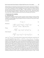
3.1

(Colour online) Behavior of the concurrence as a function of time with s = 0.5
(solid, black line) and s = 1 (dashed, red line). Inset shows the concurrence
at s = 4 (dash-dotted, orange line) and s = 6 (short-dashed, blue line) respectively. Here we set !0 = 0.1, !c = 20,

3.2

= 1 and g = 0.01. . . . . . . . .

(Colour online) Maximum concurrence with varying coupling strength g and
Ohmicity parameter s. Here !0 = 0.1, !c = 2 and

3.3

47

= 1. . . . . . . . . . . .

48

Variation of (t) with respect to Ohmicity parameter s at finite long time
t = 500 from s = 3 to s = 3.2. The inset shows the variation between s = 1.2
to s = 6. Here !0 = 0.1, !c = 2,

3.4

= 1 and g = 0.005.

. . . . . . . . . . . .

50

Variation of maximum concurrence Cmax with respect to Ohmicity parameter
s from s = 1 to s = 4 for varying values of ". Other parameters used are
!c = 50, !0 = 0.1,

= 1 and g = 0.01. Here the lines showing the pure

dephasing case and " = 0.01 are almost indistinguishable, while the di↵erence
between the pure dephasing case and " = 0.08 is also not very appreciable. .
iv

51


LIST OF FIGURES
3.5

(Colour online) Evolution of concurrence for s = 1 (solid, black line) and
s = 3 (dashed, red line). We set !0 = 0.1 and use !c = 20 for s = 1 and
!c = 2 for s = 3. Also, we have g = 0.005 and

= 1, and p1 = p3 = 0.9,

p2 = p4 = 0.1. We note that for the sub-Ohmic case, s = 0.5, the concurrence

remains zero throughout, hence is not plotted here. The inset shows the long
time evolution for s = 3. Here we note that there is a finite time interval
between each cycle of revival of entanglement. . . . . . . . . . . . . . . . . .

3.6

(Colour online) Evolution of purity for the mixed state given by Eq. (3.45).
Parameters used are same as Fig. 3.5. . . . . . . . . . . . . . . . . . . . . . .

3.7

52

(Colour online) Variation of maximum concurrence with respect to

53

for s =

3.1. The inset shows the variation of maximum concurrence with respect to
and s. Here g = 0.03, !0 = 0.1 and !c = 2. If !0 is in the GHz regime (for
instance, trapped ions), then

= 1 corresponds to a temperature in the µK

regime. . . . . . . . . . . . . . . . . . . . . . . . . . . . . . . . . . . . . . . .

3.8

54

(Colour online) Concurrence using F (!, !c ) = exp (!/!c )2 at s = 0.5 (solid,
black line), s = 1 (dashed, red line), s = 4 (dash-dotted, orange line) and
s = 6 (short-dashed, blue line) respectively. Parameters used are !c = 50,
!0 = 0.1,

3.9

= 1 and g = 0.01. . . . . . . . . . . . . . . . . . . . . . . . . . .

56

(Colour online) Concurrence at !c = 10 (solid, black line) and !c = 50 (dash,
blue line). Parameters used are s = 4, !0 = 0.1,

= 1 and g = 0.01. . . . . .

57

3.10 (Colour online) Comparison between our results using (a) our numerical program based on the master equation in Eq. (2.13) and (b) the results in Ref.
[136]. . . . . . . . . . . . . . . . . . . . . . . . . . . . . . . . . . . . . . . . .
v

58


LIST OF FIGURES
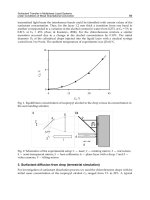
4.1

(Colour Online) Coherent spin state (left) and spin squeezed state (right) in

D E
the Bloch sphere representation. Here, the radius of the sphere gives J~ .

We observe that one main e↵ect of squeezing is that it reduces the uncertainty in one axis while increasing the uncertainty in the other (see the right
diagram). Figure is adapted from [157].

4.2

. . . . . . . . . . . . . . . . . . . .

62

(Colour online) Variation of the optimised squeezing parameter with the Ohmicity parameter s in the presence of the OAT Hamiltonian (circle, blue dotted
lines) and without the OAT Hamiltonian (square, black solid lines). Here
N = 10, g = 0.05, !0 = 0.1, !c = 10 and

4.3

= 1. . .

67

Variation of minimum ⇠S2 (t) with coupling strength g. Here N = 10, !0 = 0.1,
s = 2.5 and

5.1

= 1. For the OAT case,

= 1 and we consider the spin squeezing generated at time T = 1. 68

Schematics of the adiabatic eigenstates (represented by solid lines) and diabatic eigenstates |"i and |#i (represented by dashed lines). The regime with
the minimum gap correspond to the avoided crossing. Figure is adapted from
Ref. [85]. . . . . . . . . . . . . . . . . . . . . . . . . . . . . . . . . . . . . . .

5.2

73

(Colour online) Population P (s) of ⇢++ (s) with respect to rescaled time s
for (red, solid line)

= 1 and (blue, dashed line)

= 0.1 respectively. The

circle and star symbols represent the numerical results obtained by evolving
= 1, |A + |2 = 1 and
p
|2 = 0. The initial state of the system is given by (0) = 0.8 |+(0)i +

the master equation directly. Here we set v = 0.001,

|A+
p
0.2 | (0)i. A strong agreement between the numerical results and theory is
observed.
5.3

. . . . . . . . . . . . . . . . . . . . . . . . . . . . . . . . . . . . .

82

Transition probability of ⇢11 as a function of . The coherent state is initially
prepared in | (s0 )i = 0.8 |E1 i + 0.1 |E2 i + 0.1 |E3 i, and the mixed state is
initially in ⇢(s0 ) = 0.8 |E1 i hE1 | + 0.1 |E2 i hE2 | + 0.1 |E3 i hE3 |. Here we set
g0 = 1 and v = 10 3 . Inset shows the transition probability when the state is
prepared in a pure state | i = |E1 i. . . . . . . . . . . . . . . . . . . . . . . .
vi

86


LIST OF FIGURES
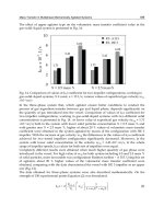
5.4

Percentage di↵erence of the transition probability of ⇢11 between the numerical
results and our theory as a function of

. The coherent state is initially

prepared in | (s0 )i = 0.4 |E1 i + 0.3 |E2 i + 0.3 |E3 i, and the mixed state is
initially in ⇢(s0 ) = 0.4 |E1 i hE1 | + 0.3 |E2 i hE2 | + 0.3 |E3 i hE3 |. Here we set
g0 = 1 and v = 10 3 . Inset shows the transition probability when the state is
prepared in a pure state | i = |E1 i. . . . . . . . . . . . . . . . . . . . . . . .

6.1

87

(Colour online) Population P (s) of state ⇢++ (s) as the system is driven with
respect to s. Blue solid lines corresponds to the analytical results and black
crosses corresponds to the results obtained by numerically evolving the Lindblad master equation directly. Here k = 0.25, v = 10 4 ,

= 1,

= 0.1,

= 1 and |A+ |2 = 0. The initial state of the system is given by
p
p
(0) = 0.8 |+(0)i + 0.2 | (0)i. Here we note that P (s) approaches zero at

|A

+|

2

around s = 0.006. Both results obtained by numerics and analytical formulas
are in strong agreement with each other. . . . . . . . . . . . . . . . . . . . . 103
6.2

(Colour online) Same as Fig. (6.1), except that

= 1. Here we note that

P (s) approaches zero at around s = 0.001. Both results obtained by numerics
and analytical formulas are in strong agreement with each other. . . . . . . . 104
6.3

(Colour online) Same as Fig. (6.1), except that

= 1, |A

+|

2

= 1 and

|A+ |2 = 1. Here we note that P (s) approaches 0.5 asymptotically instead of
zero, indicating the e↵ect of the Lindblad operators on the adiabatic probability. Both results obtained by numerics and analytical formulas are in strong
agreement with each other.
6.4

. . . . . . . . . . . . . . . . . . . . . . . . . . . 105

(Colour online) Number of pumped particles Q vs the dissipation rate
(blue, solid line)

= 1 and (red,dashed line)

described in (6.14). Here |A

+|

2

=

for

1.6 using the equation

= 1 and |A+ |2 = 0. . . . . . . . . . . . . . 106
vii


LIST OF FIGURES
6.5

(Colour online) Number of pumped particles Q vs the dissipation rate
= 2.5 using the equation described in (6.14). Here |A
0.

6.6

⇡ < k < ⇡. . . . . . . . . . . . . . . . . . . 109

(Colour online) 3D plot of the Berry curvature ⌦k,s of the QWZ model with
1.6 between 0 < s < 2⇡ and

⇡ < k < ⇡.

. . . . . . . . . . . . . . . . 110

(Colour online) 3D plot of the Berry curvature ⌦k,s of the QWZ model with
= 2.5 between 0 < s < 2⇡ and

6.9

= 1 and |A+ |2 =

(Colour online) 3D plot of the Berry curvature ⌦k,s of the QWZ model with

=
6.8

2

. . . . . . . . . . . . . . . . . . . . . . . . . . . . . . . . . . . . . . . . . 107

= 1 between 0 < s < 2⇡ and
6.7

+|

for

⇡ < k < ⇡.

. . . . . . . . . . . . . . . . . 111

(Colour online) Number of pumped particles Q vs energy bias
equation described in (6.14). Here |A
0.5) ⇡ 1.97,

+|

Q( = 2.5) ⇡ 1.46 and

2

= 1 and |A+ |2 = 0. Here,

Q( = 5.5) ⇡ 0.698.

+|

2

Q( =

. . . . . . . . . 112

6.10 (Colour online) Number of pumped particles Q vs energy bias
equation described in (6.14). Here |A

using the

using the

= 1 and |A+ |2 = 0. Here, we pre-

pare the initial state of the system to be in a superposition state of (blue solid
q
q
sin(k)
3

line) 4 + 4⇡ |+(0)i + 14 sin(k)
| (0)i and mixed state of (red dashed
⇣
⌘
⇣4⇡
⌘
sin(k)
sin(k)
3
1
line) 4 + 4⇡ |+(0)i h+(0)| + 4
| (0)i h (0)| respectively. Here,
4⇡

= 1. . . . . . . . . . . . . . . . . . . . . . . . . . . . . . . . . . . . . . . . 113

6.11 (Colour online) Number of pumped particles Q vs energy bias
equation described in (6.14). Here |A

+|

2

using the

= 1 and |A+ |2 = 0. Here, we

prepare the initial state of the system to be in a superposition state of (blue
q
q

3
k
k
solid line) 4 + 4⇡ |+(0)i + 14 4⇡
| (0)i and mixed state of (red dashed
line)

3
4

+

k
4⇡

|+(0)i h+(0)| +

1
4

k
4⇡

| (0)i h (0)| respectively. Here,

=

1.6. Here we note that maximum di↵erence of Q for a particular choice of
between superposition and mixed state is about 0.025. . . . . . . . . . . . 116
viii

LIST OF FIGURES
6.12 (Colour online) Number of pumped particles Q vs energy bias
equation described in (6.14). Here |A

+|

2

using the

= 1 and |A+ |2 = 0. Here, we

prepare the initial state of the system to be in a superposition state of (red
p
p
solid line) 0.6 |+(0)i + 0.4eik | (0)i and its mixed state counterpart (blue
dashed line) respectively. The dark yellow dashed dot line corresponds to
the contribution due to Eq.(6.10). We further note that Eq.(6.9) has no
contribution for this particular choice of initial states. Here,

=

1.6.

6.13 (Colour online)fk vs the k for the QWZ model. Here we set v = 10 4 ,

. . . 117
= 2,

= 1, |A + |2 = 1 and |A+ |2 = 0. The initial state of the system is given by
p
p
(0) = 0.8 |+(0)i + 0.2 | (0)i. A strong agreement between the numerical
results and theory is observed.

. . . . . . . . . . . . . . . . . . . . . . . . . 119

6.14 (Colour online) Number of pumped particles Q vs dephasing rate in the
h
i
(1)
(2)
1
QWZ model. Here the initial state is chosen to be 2 | k (0)i + | k (0)i ⌦
h
i
(1)
(2)
h k (0)| + h k (0)| . Other parameters used are v = 10 3 and = 0.5.

Figure is adapted from Ref. [185]. . . . . . . . . . . . . . . . . . . . . . . . . 123

6.15 (Colour online) Number of pumped particles Q vs energy bias
phase transition point

= 0 for various dephasing rate

through the

in the QWZ model.

Figure is adapted from Ref. [185]. . . . . . . . . . . . . . . . . . . . . . . . . 124

ix


Chapter

1

Introduction
1.1

What are Quantum Open Systems?

In a real world, no system is completely isolated and every system interacts with its environment. For instance, a cup of co↵ee, interacts with its surrounding and loses energy to it,
and eventually cools down and comes to an equilibrium state that is described by classical
statistical mechanics. Such kind of interaction is known as dissipation or relaxation and can
be found in both classical and quantum systems.
If we were to study the system-environment interaction in the quantum regime, there is
another phenomenon, known as decoherence1 , that will appear due to its interaction with
the environment. It refers to the destruction of superposition between two quantum state
due to its interaction with the environment. When a quantum system becomes completely
decoherent, the quantum state will then become a mixture and any information about its
superposition will be lost.
Decoherence has been widely studied for mainly two reasons: Firstly, many quantum
technologies depend on the preservation of quantum superposition and hence protecting
1

In literature, sometimes decoherence refers to the interaction with the environment whereby there is

both loss of superposition and relaxation. To avoid confusion, in subsequent chapters, we will refer such loss
of superposition as dephasing.

1


1.1. WHAT ARE QUANTUM OPEN SYSTEMS?
such superposition from decoherence becomes an important issue at hand. For instance,
many quantum applications such as quantum computing and quantum crytography rely
heavily on the coherence of quantum states, and such destruction of the states will result
in a lowered or non-efficiency of these applications. As a result, e↵orts have been devoted
to eliminate or reduce the e↵ects of decoherence on these quantum mechanical devices, for
instance, protocols such as dynamical decoupling [1–4], use of decoherence free subspace
[5, 6] or combination of protocols [7]. All these methodologies aim to preserve the quantum
state of the system, and prevent the superposition states from decaying into a mixture, due
to the influence from their environment.
More fundamentally, given the e↵ectiveness of the quantum mechanical formalism in
explaining the behaviours in the microscopic world, it becomes a question as to why macroscopic objects do not behave like a quantum object in our everyday life. In other words,
the laws governing the macroscopic and microscopic world may be di↵erent and the division
between the two worlds is known as the Heisenberg cut [8, 9]. However, it has also been proposed that such cut does not exist and that quantum mechanical properties should manifest
itself at all scales [10]. While the interpretation of quantum mechanics remains open [11, 12],
the decoherence framework nonetheless is able to provide a partial answer to the question
posed at the start of the paragraph. In a quantum mechanical setting, the environment acts
as a probe and continuously monitor the system of interest, leading to a correlation between
the system and the environment. Any information about the coherence of the system is now
quantum mechanically entangled with the infinite degrees of freedom of the environment,
hence in practice we will no longer be able to measure any information about the coherence

that is embedded in the environment. In a more technical sense, in practice we are not able
to have a complete description of the environmental degree of freedom, even if we do, the
amount of information from the environment is too much for us to make any reasonable
calculations by treating the environment and system as a closed system [13].
As a simple illustration, consider a double slit experiment using a photon. Let |
|

2i

1i

and

be the paths of the photon through slit 1 and slit 2 respectively; and |Di be the initial
2


CHAPTER 1. INTRODUCTION
state of the detector at the screen. When the photon reaches the detector, the state will now
be entangled with the detector and this is represented as follows:
1
1
p (| 1 i + | 2 i) ⌦ |Di 7! p (| 1 i ⌦ |1i + | 2 i ⌦ |2i) = | i
(1.1)
2
2
where |1i and |2i are the states of the detector detecting the photon from slit 1 and 2
respectively.
Here, if we want to obtain information about the probability distribution of the photon
on the screen, we will need to find the reduced density matrix of the photon by performing

a trace over the detector’s degree of freedom.

1
⇢photon = TrE (| i h |) = (|
2

1i h 1|

+|

2i h 2|

+|

1 i h 2 | h1|

2i + |

2 i h 1 | h2|

1i)

(1.2)

If the states of the detector are assumed to be orthogonal, the reduced density matrix
will be simplified to
1
⇢photon = TrE (| i h |) = (|
2

1i h 1|

+|

2 i h 2 |)

(1.3)

Here, we can observe that when the photon is entangled with the detector, the orthogonality of the detector states (i.e. the outcome of the detector is clearly distinguishable) will
wash out any information about the coherence of the photon. Similarly, if we were to extend
this idea and replace photons with more general particles, the detector to the environment
(say, for example, air molecules), it is rather straightforward to see that the entanglement of
the particle with the almost orthogonal degrees of freedom of the environment will always
end up washing away the coherence between the particle states.

1.2

Overview of Main Fields of Research

The study and application of open quantum system spans over a wide range of subjects,
including quantum computation [14], condensed matter physics [15–19] and biological sys3


1.2. OVERVIEW OF MAIN FIELDS OF RESEARCH
tems [20–23], to name a few. Given the wide spectrum of research areas in this topic, it is
a daunting task to list down all the topics associated with open quantum systems. Instead,
here we will note down a list of areas of research that are currently active, bearing in mind
that the list is non-exhaustive.

1.2.1

Protection of Quantum Systems

One of the major topics in the subject of open quantum system is on the control of unwanted
interactions between the system and environment. As illustrated in the previous section, the
correlation established between the environment and system will wash away the coherence of
the system, therefore protecting the system from any loss of coherence becomes an important
task at hand. In the following we will give a review of two of the main methods of protecting
the quantum system from interaction with environment, namely reservoir engineering and
dynamical decoupling.

Reservoir Engineering
The idea of reservoir engineering was first proposed by Potayos et. al. [24], whereby the
coupling between a single ion and the environment was controlled by the absorption and
spontaneous emission of the laser photon. The idea was then explicitly discussed and extended to combat decoherence in the paper by Carvalho et. al. [25]. The essential idea
of reservoir engineering is that the system is made to couple to a reservoir at which its
pointer state includes the target state of the system. The system is then made e↵ectively
decoupled from the environment by making the engineered reservoir’s coupling significantly
stronger. One of the key advantages of such form of scheme is that since the reservoir is
prepared beforehand, there is no longer an external intervention within a small time scale.
Furthermore, compared to measurement based feedback schemes, one no longer needs to
know the measurement outcome in order to control the system. However, one of the key
challenges of such engineering is to be able to find a suitable coupling such that the system
4


CHAPTER 1. INTRODUCTION
will be driven to its target state in the steady state limit. The authors in Ref. [26] tackled
the problem by finding the necessary and sufficient conditions for a unique steady state to
exist in the Lindblad formalism, whereby it can be, in principle, used to stabilise a quantum state through reservoir engineering. A scheme that was made up of a stream of two

level systems undergoing dispersive, resonant and then dispersive atom-cavity interaction
was proposed as a possible candidate for an engineered reservoir [27]. The authors then used
this reservoir and illustrated that in a cavity with finite damping time, a stabilised squeezed
state and superposition of multiple coherent component state could be created as the result
of the system-engineered reservoir coupling. The same group of authors then showed that
the engineered reservoir was fairly robust against experimental imperfections and could be
implemented in the context of microwave cavity and circuit quantum electrodynamics [28].
In Ref. [29], the authors considered a local interaction of N particles with its individual
environment by organising the system in a particular geometry, and the local interaction
will drive the system to the desired steady state. In the aspect of bosonic reservoir engineering, one can in fact tune the so called Ohmicity2 by modifying the scattering length
of the Bose-Einstein condensate (BEC) [30]. Such form of reservoir engineering has found
applications in the control of entanglement of two impurity qubits, where the authors in
Ref. [31] showed that by controlling the reservoir parameters, one could in fact produce the
rich entanglement dynamics, such as sudden death and revival, entanglement trapping and
BEC-mediated entanglement generation. As a brief remark, we note that it is the richness
in the studies of reservoir engineering described above that motivates us in our own studies
of the environmental e↵ect of entanglement and spin squeezing to be presented in Chapter
3 and 4.

Dynamical Decoupling
Another main proposal to reduce the environmental e↵ect is by performing dynamical decoupling (DD), whereby external fields are applied to the system in such a way that the
2

We will discuss more about this in Chapter 3.

5


1.2. OVERVIEW OF MAIN FIELDS OF RESEARCH
interaction term between the system and environment changes sign rapidly. This will then

result in the interaction term being averaged out to zero, thus cancelling the e↵ect of environment on the system. Such scheme was first proposed in Ref. [32], whereby the authors
proposed using pulsed DD applied at equal interval for a single qubit coupled to a quantum
environment.
A significant advancement was made when Uhrig showed that the coherence of a single
qubit can be protected up to N th order by using N aperiodic instantaneous pulses for a
pure dephasing model (dubbed as the Uhrig DD, or UDD), thus significantly reducing the
difficulty in performing DD [33]. The idea has since been extended and it was further
illustrated that such DD is independent of the choice of system-environmental coupling [34],
and it was further shown that a nested UDD sequence can in fact protect a single qubit from
both dephasing and relaxation [35]. UDD has also been implemented experimentally and
studied in Ref. [36–38].
Another direction in this problem would be to investigate the means of protecting multiple
qubits from the undesirable e↵ects of decoherence, especially since multi qubits can have
interactions of other kinds that do not exist in single qubit systems, such as sudden death
phenomenon [39, 40]. In this aspect, it has been found that even with the lack of information
about the system-environment coupling, it is still possible to construct a N pulse sequence
to protect two qubits system up to the N th order [41]. It was then further found that by
using four layers of nested pulsed UDD, one can protect a completely unknown two-qubit
state up to a high fidelity [42].
The third direction in the topic of dynamical decoupling is the use of continuous field,
rather than a pulse sequence in the process. The main advantages of a continuous pulse
sequence are that: (i) it can be more easily implemented in practice; (ii) one no longer has
to be concerned about the type of pulse sequence anymore; (iii) the problem of imperfections
in the pulse sequence due to the finite time pulse is no longer relevant. The authors in Ref.
[43] have found that one can also achieve universal protection with respect to all types
of decoherence e↵ects by using a relatively simple form of continuous DD, i.e. via local
6


CHAPTER 1. INTRODUCTION

continuous and periodic fields. It has also been found that such form of continuous DD can
in fact be used to protect and enhance spin squeezing in multi qubit systems [44].

1.2.2

Decoherence in Adiabatic Transport

As we will see in Chapter 6, adiabatic transport is a phenomenon whereby the charged
particles are being pumped through the system when it is subjected to a cycle of slow
periodic driving. In particular, Thouless [45] showed that when a one-dimensional lattice
is being driven by a slow periodic external field, the amount of charge passing through the
cross section perpendicular to the lattice will always be given by a quantised value and
can be expressed in terms of an integral of the Berry curvature when the initial state is
given by an uniformly filled Bloch band. Such form of quantised adiabatic pumping is
known to be resilient against disorder in the substrate, as well as multi-body interactions
[46]. In fact, Thouless pump has been experimentally proposed in many di↵erent setups,
such as cold atoms and photonic systems [47–56]. Furthermore, it has also been shown
recently that the non-adiabatic correction to such transport is in fact dependent on the state
preparation, whereby the correction factor scales with respect to driving speed, v, if the
bands are coherently filled, and v 2 is the band is singly filled [57].
In terms of environmental e↵ects on adiabatic transport, most of the studies thus far
have involved systems that are coupled to leads, rather than a truly open system [58, 59].
One main e↵ect of open systems in the adiabatic pumping is that the so-called time reversal
symmetry will be broken, and as a result the charge transport will become a direct current
[60]. Nonetheless, the quantum master equation approach had been utilised to study the
e↵ects of the quantum leads in the transport process. For instance, in Ref. [61], it was
demonstrated for interacting electrons in quantum dot systems, one could control the pumping by modulating the chemical potential. In the same paper, they also derived expressions
for the cumulant generating function for the pumping and found that it was related to the
geometrical Berry-phase-like quantities in parameter space. The use of quantum master
equation was further extended to an anharmonic junction model recently where the system

7


1.2. OVERVIEW OF MAIN FIELDS OF RESEARCH
interacts with two di↵erent bosonic environments [62]. In the work, the author found that
under such setup, the pumping current displays a non-trivial relationship with respect to
both the intial states, as well as the environmental parameters, and one can then optimise
the current by controlling these parameters. Similar approach was taken in Ref. [63] in the
context of single quantum dots and it was found that in the non-adiabatic regime the charge
transport is given by a trinomial distribution. However, most of the work described above
involved quantum systems coupled to two leads, and there has been a limited number of
studies involving the coupling with a general reservoir, which is the focus of our work in this
thesis.
The remaining two sections, though having no relevance to the rest of the chapters, are
discussed nonetheless as these topics have been surveyed during the formation of this thesis,
and may be still interesting for some readers.

1.2.3

Non-Markovianity in Open Quantum Systems

Historically, the modelling of open quantum systems relied on the Markovian approximation,
i.e. the memoryless e↵ect between system and environment, in order to gain analytical insight
on the system. Such neglect of the back action of the environment, while widely studied,
is proven to be inadequate in situations where the system-environment coupling is strong,
when the temperature is low and when the environment is of a finite size or structured.
However, unlike its classical counterpart, the concept of Markovianity at this stage has no
clear and uniquely model-independent definitions. It is also unclear if one should regard
the non-Markovianity as a mathematical property of the dynamical map, or as a relevant
physical quantity that evolves with time [64]. In terms of its definition, various quantitative

measures have been proposed to define non-Markovianity, with the main criteria being that
it has to be independent of the choice of the model. For example, Rivas et. al. proposed a
measure, known as the RHP measure, that was dependent on the divisibility of the quantum
dynamical map [65]. On the other hand, Breuer et. al. proposed another more physically
intuitive measure [66], the BLP measure, that was based on the fact that since the system’s
8


CHAPTER 1. INTRODUCTION
interaction with the environment will typically reduce the distinguishability of the quantum
states, any moment in time when the distinguishability increases between the quantum states
will be due to the backflow of information from the environment, and by quantifying such
amount, one can in fact measure the degree of non-Markovianity. However, at this stage there
is still no consensus on the appropriate measure to use and the suitability of the di↵erent
measures is still an open question [67–69].
Another aspect of the problem is the possibility of using the non-Markovian property as a
resource and exploiting it in quantum processes. It has been demonstrated that by exploiting
the memory time of the environment, one can in fact generate entanglement that are longlived even with the presence of environment [70]. It has also been shown that in the JaynesCumming model, the non-Markovianity of the environment can be used to speed up quantum
evolutions resulting in a shorter quantum speed limit time [71]. It has further been shown
recently [72] that such non-Markovianity is related to the so called coherence trapping of the
quantum states, where the coherence of the steady state is found to be maximised whenever
the qubit undergoes a non-Markovian dynamics. These results have further been extended
recently to include systems with initial system-environment correlation [73]. Furthermore,
it has also been proposed recently that non-Markovianity can be harnessed as a resource for
quantum technologies [74–77].

1.2.4

Aspects of Open Quantum Systems in Biological Systems

The union between quantum mechanics and biological systems is indeed one that is intriguing. For a long time, the warm and wet environment that biological systems are subjected to
has been thought to prevent any sort of quantum mechanical e↵ects from persisting, and it
is such ideas that partially explain the stability of certain molecules. However, the developments in the recent decade has shown that not only that such quantum e↵ects are important
to biological systems, but also it is paradoxically the interaction with its environment that
allows numerous biological processes to take place. One distinctive example is the energy
transfer in photosynethesis processes [21–23, 78–80]. The seminal works in Refs. [21, 79]
9