- Trang chủ >>
- Khoa Học Tự Nhiên >>
- Vật lý
Ebook Physical chemistry (4th edition) Part 2
Bạn đang xem bản rút gọn của tài liệu. Xem và tải ngay bản đầy đủ của tài liệu tại đây (6.68 MB, 491 trang )
13
Rotational and Vibrational Spectroscopy
13.1
13.2
13.3
13.4
13.5
13.6
13.7
13.8
13.9
13.10
The Basic Ideas of Spectroscopy
Einstein Coefficients and Selection Rules
Schro¨dinger Equation for Nuclear Motion
Rotational Spectra of Diatomic Molecules
Rotational Spectra of Polyatomic Molecules
Vibrational Spectra of Diatomic Molecules
Vibration–Rotation Spectra of Diatomic Molecules
Vibrational Spectra of Polyatomic Molecules
Raman Spectra
Special Topic: Fourier Transform Infrared
Spectroscopy
Molecular spectroscopy is a powerful tool for learning about molecular structure
and molecular energy levels. The study of rotational spectra gives us information
about moments of inertia, interatomic distances, and angles. Vibrational spectra
yield fundamental vibrational frequencies and force constants. Electronic spectra
yield electronic energy levels and dissociation energies.
The types of spectroscopic transitions that can occur are limited by selection
rules. As in the case of atoms, the principal interactions of molecules with electromagnetic radiation are of the electric dipole type, and so we will concentrate on
them. Magnetic dipole transitions are about 10 5 times weaker than electric dipole
transitions, and electric quadrupole transitions are about 108 times weaker. Although the selection rules limit the radiative transitions that can occur, molecular
collisions can cause many additional kinds of transitions. Because of molecular
collisions the populations of the various molecular energy levels are in thermal
equilibrium.
13.1 The Basic Ideas of Spectroscopy
13.1
THE BASIC IDEAS OF SPECTROSCOPY
When an isolated molecule undergoes a transition from one quantum eigenstate
with energy E1 to another with energy E2 , energy is conserved by the emission or
absorption of a photon. The frequency of the photon is related to the difference
in energies of the two states by Bohr’s relation,
h ϵ hc˜ ͉ סE1 Ϫ E2 ͉
(13.1)
where we have used the symbol ˜ ( ס1/) introduced in Chapter 9 for the transition energy in wave numbers (SI unit mϪ1 , but usually cmϪ1 is used). The wave
number ˜ is the number of waves per unit length. If E1 Ͼ E2 , the process is photon emission; if E1 Ͻ E2 , the process is photon absorption. The frequency range
of photons, or the electromagnetic spectrum, is classified into different regions according to custom and experimental methods as outlined in Table 13.1. By measuring the frequency of the photon, we can learn about the eigenstates of the
molecule being studied. This is called molecular spectroscopy.
The frequency of the photon in the absorption or emission process often tells
us the kinds of molecular transitions that are involved. In the radio-frequency
region (very low energy), transitions between nuclear spin states can occur
(see Chapter 15). In the microwave region, transitions between electron spin
states in molecules with unpaired electrons (Chapter 15) and, in addition, transitions between rotational states can take place. In the infrared region, transitions
between vibrational states take place (with and without transitions between rotational states). In the visible and ultraviolet regions, the transitions occur between
electronic states (accompanied by vibrational and rotational changes). Finally, in
the far ultraviolet and X-ray regions, transitions occur that can ionize or dissociate
molecules.
Table 13.1
␥ rays
X-rays
Vacuum UV
Near UV
Visible
Near IR
Mid IR
Far IR
Microwaves
Radio waves
Regions of the Electromagnetic Spectrum
Wavelength
in Vacuo, 0
Wave Number
in Vacuo, ˜
Frequency,
Photon Energy,
h
Molar Energy,
NA h
10 pm
10 nm
200 nm
380 nm
780 nm
2.5 m
50 m
1 mm
100 mm
1000 mm
109 cmϪ1
106 cmϪ1
50.0 ϫ 103 cmϪ1
26.3 ϫ 103 cmϪ1
12.8 ϫ 103 cmϪ1
4.00 ϫ 103 cmϪ1
200 cmϪ1
10 cmϪ1
0.1 cmϪ1
0.01 cmϪ1
30.0 EHz
30.0 PHz
1.50 PHz
789 THz
384 THz
120 THz
6.00 THz
300 GHz
3.00 GHz
300 MHz
19.9 ϫ 10Ϫ15 J
19.9 ϫ 10Ϫ18 J
993 ϫ 10Ϫ21 J
523 ϫ 10Ϫ21 J
255 ϫ 10Ϫ21 J
79.5 ϫ 10Ϫ21 J
3.98 ϫ 10Ϫ21 J
199 ϫ 10Ϫ24 J
1.99 ϫ 10Ϫ24 J
0.199 ϫ 10Ϫ24 J
12.0 GJ/mol
12.0 MJ/mol
598 kJ/mol
315 kJ/mol
153 kJ/mol
47.9 kJ/mol
2.40 kJ/mol
120 J/mol
12.0 J/mol
1.2 J/mol
IR, infrared; UV, ultraviolet. The abbreviations for powers of 10 are given inside the back cover of the book. Source: IUPAC Report,
“Names, Symbols, Definitions, and Units for Quantities in Optical Spectroscopy,” 1984.
Example 13.1 Calculation of the energy of light
Calculate the energy in joules per quantum, electron volts, and joules per mole of photons
of wavelength 300 nm.
459
460
Chapter 13
Rotational and Vibrational Spectroscopy
h ס
hc
(6.62 ϫ 10Ϫ34 J s)(3 ϫ 108 m sϪ1 )
ס
ס6.62 ϫ 10Ϫ19 J
(300 ϫ 10Ϫ9 m)
( ס6.62 ϫ 10Ϫ19 J)/(1.602 ϫ 10Ϫ19 J eVϪ1 ) ס4.13 eV
NA h ( ס6.02 ϫ 1023 molϪ1 )(6.62 ϫ 10Ϫ19 J) ס398 kJ molϪ1
We shall see that the energy eigenvalues of a molecule can be written as
E סEr םEv םEe
(13.2)
where Er is the rotational energy, Ev the vibrational energy, and Ee the electronic
energy. When the molecule undergoes a transition to another state with the emission or absorption of a single photon of frequency , then
h ( סErЈ Ϫ ErЈЈ) ( םEvЈ Ϫ EvЈЈ) ( םEeЈ Ϫ EeЈЈ)
(13.3)
The primes refer to the state of higher energy and the double primes to the state
of lower energy.
The classification of the various regions of the electromagnetic spectrum by
the type of transition given above is possible because, in general,
ErЈ Ϫ ErЈЈ ϽϽ EvЈ Ϫ EvЈЈ ϽϽ EeЈ Ϫ EeЈЈ
(13.4)
That is, electronic energy level differences are much greater than vibrational energy level differences, which are much greater than rotational energy level differences. Electronic transitions are often in the visible and ultraviolet part of the
spectrum; vibrational transitions are in the infrared, and rotational transitions are
in the far infrared and microwave regions.
13.2
EINSTEIN COEFFICIENTS AND SELECTION RULES
The spectrum of a molecule consists of a series of lines at the frequencies corresponding to all the possible transitions. Let us consider the transition from state
1 to state 2. The strength or intensity of a spectral line depends on the number of
molecules per unit volume Ni that were in the initial state (the population density
of that state) and the probability that the transition will take place. Einstein postulated that the rate of absorption of photons is proportional to the density of the
electromagnetic radiation with the right frequency. The radiant energy density is
the radiant energy per unit volume, so it is expressed in J mϪ3 . (See Section 9.16.)
The spectral radiant energy density as a function of frequency is the measure
of the radiant energy of a particular frequency; it is given by
סd /d
(13.5)
Ϫ3
Thus, is expressed in J s m . The energy density at the frequency required to excite atoms or molecules from E1 to E2 is represented by (12 ). Thus Einstein’s postulate about the rate of absorption of photons is summarized by the rate equation
dt
dN1
סϪB12 (12 )N1
(13.6)
abs
where B12 is the Einstein coefficient for stimulated absorption. The SI unit for
B12 is m kgϪ1 . (Note that N1 can be taken as dimensionless or expressed in mϪ3 .)
There is a minus sign because N1 decreases when electromagnetic radiation is
absorbed. Note that dN1 /dt סϪdN2 /dt .
13.2 Einstein Coefficients and Selection Rules
Excited atoms or molecules do not remain in excited states indefinitely, and
Einstein postulated two processes for their return to the initial state, namely, spontaneous emission and stimulated emission, as illustrated in Fig. 13.1. The rate of
spontaneous emission is given by (here N2 is the population density of state 2)
dt
סϪA21 N2
1
2
where A21 is the Einstein coefficient for spontaneous emission. The SI unit for A21
is sϪ1 . The rate of spontaneous emission is independent of the radiation density,
and the radiation is emitted in random directions with random phases.
Stimulated emission is quite different in that its rate is proportional to (12 ),
and the electromagnetic wave that is produced adds in phase and direction (i.e.,
coherently) to the stimulating wave. The rate of stimulated emission is indicated
by the rate equation
סϪB21 (12 )N2
A21N2
1
Spontaneous emission
2
B21N2 ρν∼ (ν∼12)
(13.8)
stim
1
where B21 is the Einstein coefficient for stimulated emission. The interesting
feature in stimulated emission is that it amplifies the radiation density. According to equation 13.8, incident light with frequency 12 causes more radiation to
be produced with exactly the same frequency and direction as long as there are
molecules in state 2. As we will discuss later in more detail, this is the basis for
a laser, which is the acronym for “light amplification by stimulated emission of
radiation.”
Equations 13.6–13.8 have been written for the three separate processes, but
of course all three can occur in a system at the same time so that the whole rate
equation is
dN1
dN2
סϪ
סϪB12 (12 )N1 םA21 N2 םB21 (12 )N2
dt
dt
(13.9)
This rate equation leads to several interesting conclusions. The first is that the
three Einstein coefficients are related to each other. This can be seen by considering the equilibrium situation in which dN1 /dt סϪdN2 /dt ס0. When the system
is in equilibrium, equation 13.9 can be solved for the equilibrium spectral radiant
energy density (12 ) to obtain
(12 ) ס
B12N1 ρν∼ (ν∼12)
(13.7)
spont
dN2
2
Stimulated absorption
dN2
dt
461
A21
(N1 /N2 )B12 Ϫ B21
(13.10)
When the system is in equilibrium, the ratio N1 /N2 is given by the Boltzmann
distribution (Section 16.1). When E2 is the energy of the higher level and E1 is the
energy of the lower level, the Boltzmann distribution shows that
N2 סN1 eϪ(E2 ϪE1 )/kT
(13.11)
Since E2 Ϫ E1 is positive, most of the atoms or molecules will be in the lower
energy level at thermal equilibrium. If the system is exposed to electromagnetic
radiation with frequency 12 , where h12 סE2 Ϫ E1 , the equilibrium distribution
can be written as
N2
סexp(Ϫh12 /kB T )
N1
(13.12)
Stimulated emission
Figure 13.1 Definition of Einstein
coefficients.
462
Chapter 13
Rotational and Vibrational Spectroscopy
Replacing N1 /N2 in equation 13.10 with the Boltzmann distribution yields
A21
(12 ) ס
(13.13)
B12 eh12 /kB T Ϫ B21
This equation must be in agreement with Planck’s blackbody distribution law
(equation 9.2),
8h (12 /c )3
(12 ) סh /kT
(13.14)
Ϫ1
e 12
because they both apply to a system at equilibrium. Comparison of equation 13.13
with equation 13.14 indicates that
B12 סB21
(13.15)
and
A21 ס
3
8h12
B21
c3
(13.16)
Thus a measurement of any one of the three Einstein coefficients yields all three.
The second conclusion from equation 13.9 is that the time course of the irradiation can be calculated. Since B12 סB21 , these symbols can be replaced by B, and
since there is no A12 , A21 can be replaced by A. N1 can be replaced by Ntotal Ϫ N2 ,
where Ntotal סN1 םN2 , and equation 13.9 can be integrated (see Problem 13.4)
to obtain
N2
B (12 )
ס
(13.17)
Θ1 Ϫ exp ͕Ϫ[A ם2B (12 )]t ͖Ι
Ntotal
A ם2B (12 )
At t ס0, there are no excited atoms or molecules. But if the radiation density is
held constant, N2 /Ntotal rises to an asymptotic value of B (12 )/[A ם2B (12 )].
The interesting thing about this asymptotic value is that it is necessarily less than
1/2 because A Ͼ 0. This means that irradiation of a two-level system can never
put more atoms or molecules in the higher level than in the lower level. This may
be a surprise, but the significance of the conclusion is that laser action cannot be
achieved with a two-level system. In order to obtain laser action, stimulated emission must be greater than the rate of absorption so that amplification of radiation
of a particular frequency is obtained. This requires that
B21 (12 )N2 Ͼ B12 (12 )N1
(13.18)
Since B12 סB21 , laser action can be obtained only when N2 Ͼ N1 . This situation is referred to as a population inversion. The way population inversion can be
achieved is discussed in the next chapter.
Quantum mechanics provides the means to calculate Anm (and Bnm ) between
states n and m in terms of the transition dipole moment. Anm (and Bnm ) is proportional to the square of the transition dipole moment nm , defined by
nm ס
Ύ ˆ
ء
n
m
d
(13.19)
where ˆ is the quantum mechanical dipole moment operator for the molecule:
ˆ סΑ qi ri
(13.20)
i
where the sum is over all the electrons and nuclei of the molecule, qi is the charge,
and ri is the position of the ith charged particle. To understand how the transition
13.2 Einstein Coefficients and Selection Rules
moment enters, we can think of the molecule interacting with the electric field of
the radiation because of a transient or fluctuating dipole moment given by equation 13.19.
From equation 13.19, we see that if the transition dipole moment vanishes
(usually because of symmetry), the spectral line has no intensity. The rules governing the nonvanishing of nm are called selection rules, and these allow us to
make sense out of observed molecular spectra.
If the transition moment from state n to state m is nonzero and there is enough
population in the initial state, then the spectral line will be seen in the spectrum.
The quantum mechanical derivation of the relationship between the Einstein coefficients and the transition probability is too advanced for this book;* however,
the final results are given here. When the ground state and excited states have
degeneracies of g1 and g2 , the Einstein coefficient A is given by
Aס
16 3 3 g1
͉12 ͉2
3⑀0 hc 3 g2
(13.21)
This equation indicates that the rate of spontaneous emission, A12 N2 , increases
rapidly with frequency; as a matter of fact, this rate is negligible in the microwave
and infrared regions, and so only absorption spectra are measured. In the visible
and ultraviolet regions spontaneous emission is significant, and both emission and
absorption spectra are measured. The Einstein coefficient B is given by
B ס
2 2 g1
͉12 ͉2
3h 2 ⑀0 g2
(13.22)
If the rate of spontaneous emission is negligible, the net rate of absorption is
given by
rate2 Y 1 סB21 N1 ˜ (˜ 21 ) Ϫ B12 N2 ˜ (˜ 21 ) ( סN1 Ϫ N2 )B˜ (˜ 21 ) (13.23)
This shows that if the populations of the two states are equal, there will be no net
absorption of radiation.
We can also think of A12 as a measure of the lifetime of state 2. Consider
molecules in (excited) state 2 with no radiation field present (and so no stimulated
emission). The molecules will make a transition to state 1, emitting a photon frequency ˜ 21 , with a probability A12 N2 . Every time this occurs, N2 decreases. After
a time t , the number of molecules per unit volume in state 2 is given by
N2 (t ) סN2 (0) eϪA12 t סN2 (0) eϪt /
(13.24)
Ϫ1
where we have defined the lifetime סA12
. Actually, if a molecule in state 2 can
also make transitions to states 3, 4, . . . (with photons of frequency ˜ 23 , ˜ 24 , . . .),
then the total radiative lifetime is given by
1
סΑ A 2i
i
(13.25)
If other decay processes besides radiative transitions are possible (such as nonradiative transitions) we must add those rates to equation 13.25 to get the total
decay rate (inverse lifetime).
*See J. Steinfeld, Molecules and Radiation. Cambridge, MA: MIT Press, 1985.
463
464
Chapter 13
Rotational and Vibrational Spectroscopy
Example 13.2 Radiative lifetimes and transition moments
The radiative lifetime of a hydrogen atom in its first excited level (2p) is 1.6 ϫ 10Ϫ9 s. What
is the magnitude of the electronic transition moment 21 for this transition? The degeneracy g2 of the 2p level is 3. [˜ ( ס2.46 ϫ 1015 sϪ1 )/(2.998 ϫ 108 m sϪ1 ) ס8.21 ϫ 106 mϪ1 .]
1/2
21 ס
΄
3h⑀0 g2
3
16 3 ˜ 21
΅
ס
΄
(3)(6.626 ϫ 10Ϫ34 J s)(8.854 ϫ 10Ϫ12 C 2 NϪ1 mϪ2 )(3)
16 3 (8.21 ϫ 106 mϪ1 )3 (1.6 ϫ 10Ϫ9 s)
1/2
΅
ס10.9 ϫ 10Ϫ30 C m
A dipole moment of this magnitude corresponds to a distance from the proton to the electron of
r ס
10.9 ϫ 10Ϫ30 C m
1.6 ϫ 10Ϫ19 C
ס68.1 pm
This transition dipole moment can be visualized as the movement of an electron
68.1 pm/52.9 pm ס1.29 Bohr radii.
13.3
¨
SCHRODINGER
EQUATION FOR NUCLEAR MOTION
We saw in Chapter 11 that the Schro¨dinger equation for a molecule can be treated
in the Born–Oppenheimer approximation so that the electronic Hamiltonian is
that for fixed nuclei, while the Hamiltonian for nuclear motion contains the kinetic energy operator of the nuclei and the electronic energy (as a function of the
nuclear coordinates) as the potential energy operator:
2
h¯
2
םE(R )
Hˆ סϪ ٌR
2
(13.26)
In the absence of external fields (such as magnetic or electric fields), the potential
energy term E(R ) can depend only on the relative positions of the nuclei, not on
where the molecule is placed or on the orientation of the molecule in space.
The kinetic energy operator consists of the kinetic energy of the center of
mass (leading to the translational energy of the molecule), the kinetic energy associated with rotational motion, and the kinetic energy of the vibrational motion.
Thus, to a very good approximation, we may write
H סHtr םHrot םHvib
(13.27)
where the translational and rotational Hamiltonians contain only kinetic energy
terms, while the vibrational Hamiltonian contains E(R ), the potential energy depending on the internuclear distances. These internuclear distances are the vibrational coordinates of the molecule.
If the Hamiltonian is the sum of three terms, one for each kind of motion,
then the wavefunction can be written as a product of wavefunctions:
סtr rot vib
(13.28)
13.4 Rotational Spectra of Diatomic Molecules
The Schro¨dinger equations for the three terms are
Hˆ tr tr סEtr tr
Hˆ rot rot סErot rot
Hˆ vib vib סEvib vib
(13.29)
(13.30)
(13.31)
The translational wavefunction is that for a free particle (or particle in a very large
box) with a mass equal to the mass of the molecule. The translational eigenvalues
are very closely spaced and cannot be probed in molecular spectroscopy, so we
will neglect them in our discussions.
To understand the number of coordinates required to describe a polyatomic
molecule, consider the following. The total number of coordinates needed to describe the locations of the N atoms in a molecule is 3N. However, to describe
the internal motions in a molecule, we are not interested in its location in space,
and so the three coordinates required to specify the position of the center of mass
of the molecule can be subtracted, leaving 3N Ϫ 3 coordinates. To describe the
rotational motions of a molecule, we are interested in its orientation in a coordinate system. The orientation of a diatomic or linear molecule with respect to a
coordinate system requires two angles, so this leaves 3N Ϫ 5 coordinates to describe the internal motions. The orientation of a nonlinear polyatomic molecule
with respect to a coordinate system requires three angles, so this leaves 3N Ϫ 6
coordinates to describe the internal motions. These 3N Ϫ 5 or 3N Ϫ 6 internal
motions are referred to as vibrational degrees of freedom.
To sum up, for a diatomic molecule, Hˆ rot depends only on two angles, and
(see equation 9.153); Hˆ vib depends only on R , the internuclear separation. For
polyatomic molecules, Hˆ vib is more complex, depending on 3N Ϫ 6 coordinates
for nonlinear molecules and 3N Ϫ 5 coordinates for linear molecules. We will now
turn to a description of the rotational and vibrational eigenstates of both diatomic
and polyatomic molecules.
13.4
ROTATIONAL SPECTRA OF DIATOMIC MOLECULES
To a first approximation the rotational spectrum of a diatomic molecule may be
understood in terms of the Schro¨dinger equation for rotational motion of the rigid
rotor (equation 9.142). The wavefunctions are the spherical harmonics YJM(, ),
and there are two quantum numbers J and M for molecular rotation. The energy
eigenvalues are given by
Er ס
h¯ 2
J (J ם1)
2I
J ס0, 1, 2, . . .
M סϪJ, . . . , 0, . . . , םJ
(13.32)
where I is the moment of inertia (Section 9.11). Since the energy does not depend
on M , the rotational levels are (2 J ם1)-fold degenerate.
In spectroscopy it is standard to express the energies of various levels in wave
numbersbydividing E by hc andreferringtothesevaluesas termvalues. Termvalues
areusuallygivenincmϪ1 ,buttheSIunitforatermvalueismϪ1 .Atildewillbeusedto
indicate the wave numbers in cmϪ1 . Rotational term values are represented by F˜ (J )
סEr /hc , so that the rotational term values for a diatomic molecule are given by
Er
J (J ם1)h
F˜ (J ) ס
ס
סJ (J ם1)B˜
hc
8 2 Ic
(13.33)
465
466
Chapter 13
Rotational and Vibrational Spectroscopy
where the rotational constant is written
h
8 2 Ic
B˜ ס
(13.34)
where c is the speed of light, 2.998 ϫ 1010 cm sϪ1 . The rotational energy levels for
a rigid diatomic molecule are given in Fig. 13.2 in terms of the rotational constant.
According to the Born–Oppenheimer approximation (Section 11.1), the
wavefunction for a molecule in the electronic state e , the vibrational state v ,
and having a particular set of rotational quantum numbers JM can be written as
a product e v JM . The transition moment for an electric dipole transition from
a rotational state JM to a rotational state J ЈM Ј of the same electronic state is
therefore given by
ΎΎΎ Ј
ء ء ء
ˆ e v JM
e v J MЈ
de drot dvib
(13.35)
where ˆ is the dipole moment operator. Note that only the rotational function
(e)
has changed in the transition. The permanent dipole moment 0 of a molecule
in this electronic state is equal to the expectation value of the operator over
the wavefunction for the electronic state:
Ύ ˆ d
ء
e
(e)
0 ס
e
(13.36)
e
Thus, equation 13.35 becomes
ΎΎ Ј
(e)
ء ء
v J M Ј 0 v JM
drot dvib
Quantum
number
Energy
∼
20B
J=4
(13.37)
Relative
population
∼
9e– 20h cB/kt
∼
8B
J=3
∼
12B
∼
7e– 12h cB/kt
∼
6B
∼
5e– 6h cB/kt
∼
2B
∼
3e– 2h cB/kt
∼
1e–h cB/kt
∼
6B
E
J=2
∼
4B
∼
2B
J=1
J=0
J=1
2
∼
2B
0
0
3
∼
2B
4
∼
2B
ν
Figure 13.2 Rotational levels for a rigid diatomic molecule and the absorption spectrum
that results from ⌬ J ס1. The energies and relative populations of the two levels are indicated on the right. The transitions are labeled by the upper of the two J values involved.
Note that the degeneracies of the levels have been taken into account in the population,
and the intensities of the lines depend on the relative populations.
13.4 Rotational Spectra of Diatomic Molecules
The integral over the vibrational coordinate yields the permanent dipole moment
in that particular vibrational state. For simplicity, we will write it as 0 , so that the
final result for the integral is
Ύ Ј
ء
J M Ј 0 JM
drot
(13.38)
A molecule has a rotational spectrum only if this integral is nonzero. Thus, the
gross selection rule for rotational spectra is that a molecule must have a permanent
dipole moment to emit or absorb radiation in making a transition between different
states of rotation. This is expected from the fact that a rotating dipole produces
an oscillating electric field that can interact with the oscillating field of a light
wave. A homonuclear diatomic molecule such as H2 or O2 does not have a dipole
moment, so it does not show a pure rotational spectrum. Heteronuclear diatomic
molecules do have dipole moments, so they do have rotational spectra. Polyatomic
molecules are discussed in the next section. To find the specific selection rules we
need to find the conditions on the quantum numbers that make the integral in
equation 13.38 nonzero. For a linear molecule it can be shown that the transition
moment is nonzero for
⌬ J סϮ1
⌬M ס0, Ϯ1
This selection rule may be understood in the same way as that for atoms (Section
10.14). Since a photon has one unit of angular momentum, and angular momentum must be conserved in emission or absorption, the angular momentum of a
molecule must change by a compensating amount.
The frequencies ˜ of the absorption lines due to J y J ם1 are given by the
difference between rotational term values (equation 13.33):
˜ סF˜ (J ם1) Ϫ F˜ (J )
([ סJ ם1)(J ם2) Ϫ J (J ם1)]B˜
ס2B˜ (J ם1)
J ס0 , 1, 2, . . .
(13.39)
As shown in Fig. 13.2, the frequencies of the successive lines in the rotational spectrum are given by 2B˜ , 4B˜ , 6B˜ , . . . . Thus, there is a series of equally spaced lines
with separations of 2B˜ . A separate series of lines is found for each isotopically different species of a given molecule, because the moments of inertia of isotopically
substituted molecules are different.
We have been talking about diatomic molecules as if they are rigid rotors,
but of course they are not. As the rotational motion increases, the chemical bond
stretches due to centrifugal forces, the moment of inertia increases, and, consequently, the rotational energy levels come closer together. This may be taken into
account by adding a term to equation 13.33:
Er
F˜ (J ) ס
סB˜ J (J ם1) Ϫ D˜ J 2 (J ם1)2
hc
(13.40)
The quantity D˜ is the centrifugal distortion constant in wave numbers. When centrifugal distortion is taken into account, the frequencies ˜ of the absorption lines
due to J y J ם1 are given by
˜ סF˜ (J ם1) Ϫ F˜ (J )
ס2B˜ (J ם1) Ϫ 4D˜ (J ם1)3
J ס0, 1, 2, . . .
(13.41)
467
468
Chapter 13
Rotational and Vibrational Spectroscopy
The moment of inertia of a diatomic molecule also depends on its vibrational state because of the anharmonicity of vibrational motion. Since molecules
are generally in their ground vibrational state at room temperature, we do not
have to take this into account in considering pure rotational spectra; however, we
will have to take it into account by an extension of equation 13.41 in discussing
vibration–rotation spectra.
Example 13.3 Internuclear distance from rotational spectra
In early measurements of the pure rotational spectrum of H35 Cl, Czerny found that the
wave numbers of absorption lines are given by
˜ ( ס20.794 cmϪ1 )(J ם1) Ϫ (0.000 164 cmϪ1 )(J ם1)3
where J is the quantum number of the lower state. What is the internuclear distance in
H35 Cl? What is the value of the centrifugal distortion constant?
From equation 13.41, B˜ ס10.397 cmϪ1 . Since
B˜ ס
h
h
ס
8 2 cI
8 2 cR02
we have
Ί 8 c B˜
ס
Ί 8 (2.998 ϫ 10
R0 ס
h
2
2
10
6.626 ϫ 10Ϫ34 J s
cm
68 ϫ 10Ϫ27 kg)(10.397 cmϪ1 )
sϪ1 )(1.626
ס129 pm
(The reduced mass of H35 Cl is given in Example 9.21.) The centrifugal distortion constant
is given by
D˜ ס14 (0.000 164 cmϪ1 ) ס4.1 ϫ 10Ϫ5 cmϪ1
We have discussed the selection rules that determine the transitions that can
give rise to absorption or emission, but we already noted that there is another factor that determines the observed intensities, namely, the population of the initial
state given by the Boltzmann distribution (equations 13.11 and 16.2). The fraction
fi of the molecules in the ith energy state is given by
fi ס
eϪ⑀i /kT
eϪ⑀i /kT
ס
/
⑀
kT
Ϫ
q
Αi e i
(13.42)
where q is the denominator. If the energy of a state is large compared with kT , the
probability of finding a molecule in that state at equilibrium will be small. Because
of degeneracy (Section 9.7), many states of a molecule may have the same energy,
and these degenerate states make up the energy level. When energy levels are
used, the Boltzmann distribution can be written
fi ס
gi eϪ⑀i /kT
Α i gi eϪ⑀i /kT
(13.43)
13.5 Rotational Spectra of Polyatomic Molecules
where gi is the degeneracy (Section 9.7) of the ith level. As discussed earlier, the
component of the angular momentum in a particular direction is equal to MJh¯,
where MJ may have values of J, (J Ϫ 1), . . . , 0, . . . , ϪJ , where J is the rotational
quantum number. Thus, there are in all 2 J ם1 different possible states with quantum number J . In the absence of an external electric or magnetic field the energies
are identical for these various sublevels, and so the Jth energy level is said to have
a degeneracy of 2 J ם1. The rotational energy in the absence of an external elec˜ in equation 13.41, is given by ⑀i סhcBJ(J ם1)
tric or magnetic field, ignoring D
so that, using equation 13.42, the fraction of molecules in the Jth rotational level
is given by
fJ ס
(2 J ם1) eϪ[hcJ(J ם1)B ]/kT
q
(13.44)
According to this equation, the number of molecules in level J increases with J
at low J values, goes through a maximum, and then, because of the exponential
term, decreases as J is further increased. The lines in the spectrum at the bottom of
Fig. 13.2 have been labeled with the rotational quantum number J of the upper of
the two states involved. The intensities of the lines are proportional to the populations in the lower state involved in the transition.
For molecules with larger moments of inertia I , the rotational energies
are smaller, in fact, small compared with kT . The quantum numbers may become quite large before eϪ⑀ J /kT becomes appreciably different from unity. For
small quantum numbers populations are proportional to the degeneracies, since
eϪ⑀ J /kT Ϸ 1 for ⑀J ϽϽ kT .
There is a complication in rotational spectroscopy that we will not be able
to discuss. The statistics of nuclear spin affect the number of degenerate states at
each J level, and therefore the intensities of the rotational lines. The use of the
Boltzmann distribution alone is an oversimplification.*
Although homonuclear diatomic molecules do not have permanent electric
dipole moments and do not exhibit pure rotational spectra, they do show rotational Raman spectra (Section 13.9), and their electronic and vibrational spectra
show rotational fine structure.
13.5
ROTATIONAL SPECTRA OF POLYATOMIC MOLECULES
For the treatment of its pure rotational spectrum we may consider a polyatomic
molecule to be a rigid framework with fixed bond lengths and angles equal to their
mean values. For a polyatomic molecule the moment of inertia about a particular
axis that passes through the center of mass of the molecule is simply the sum of
the moments due to the various nuclei about that axis:
I סΑ mi Ri2
(13.45)
i
where Ri is the perpendicular distance of the nucleus mass mi from the axis.
The rotation of a polyatomic molecule can be described in terms of moments
of inertia taken relative to three mutually perpendicular axes. The moment about
the z axis is
Iz סΑ mi (xi2 םyi2 )
i
*See the references at the end of the chapter, such as Herzberg.
(13.46)
469
470
Chapter 13
Rotational and Vibrational Spectroscopy
Y(b)
c
X(a)
a
b
Z(c)
Figure 13.3 Momental ellipsoid with symmetry axes a, b, and c. The a, b, and c axes are
fixed with respect to the molecule and rotate with it.
and Ix and Iy are defined similarly. In addition, there are three products of inertia
that are defined like
Ixy סIyx סΑ mi xi yi
(13.47)
i
For any rigid molecule it is possible to choose a set of perpendicular axes that
pass through the center of mass such that all products of inertia vanish. These
three Cartesian axes, which are illustrated in Fig. 13.3, are called the principal axes,
and the moments of inertia about these axes are called the principal moments of
inertia Ia , Ib , and Ic . The axes are designated by a, b, and c and are fixed with
respect to the molecule and rotate with it. The principal moments of inertia about
these axes are always labeled so that Ia Յ Ib Յ Ic . The principal axes can often
be assigned by inspecting the symmetry of the molecule. The momental ellipsoid
is constructed as follows. Lines are drawn from the center of mass of the molecule
in various directions with length proportional to (I␣ )Ϫ1/2 , where I␣ is the moment
of inertia about that line as an axis. Any symmetry operation of a molecule must
apply to its momental ellipsoid.
The principal moments of inertia are used to classify molecules, as shown in
Table 13.2. If all three principal moments of inertia are equal, the molecule is a
spherical top. If two principal moments are equal, the molecule is a symmetric
top. A molecule is a prolate top (cigar shaped) if the two larger moments are
equal. The molecule is an oblate top (discus shaped) if the two smaller moments
are equal. The molecule is an asymmetric top if all three principal moments are
unequal.
The quantum mechanical Hamiltonian operator for the rotational motion of
polyatomic molecules is found by first writing the classical mechanical energy in
terms of angular momentum operators. Since we know how to convert classical
angular momentum to its quantum mechanical form, we can then find the quantum Hamiltonian and solve the Schro¨dinger equation. The last part turns out to
be straightforward for all the cases except the asymmetric top. We will not discuss
the latter.
In classical mechanics the rotational energy of a rotor with one degree of
freedom is
13.5 Rotational Spectra of Polyatomic Molecules
Table 13.2
Classification of Polyatomic Molecules According to
Their Moments of Inertia
Moments of
Inertia
Type of Rotor
Examples
Ib סIc , Ia ס0
Ia סIb סIc
Ia Ͻ Ib סIc
Ia סIb Ͻ Ic
Ia Ib Ic
Linear
Spherical top
Prolate symmetric top
Oblate symmetric top
Asymmetric top
HCN
CH4 , SF6 , UF6
CH3 Cl
C6 H6
CH2 Cl2 , H2 O
Er ס12 I 2 ס
(I )2
L2
ס
2I
2I
(13.48)
where is the angular velocity in radians per second, I is the moment of inertia,
and L is the angular momentum. For an object that can rotate in three dimensions
the classical expression for the rotational kinetic energy is
Er ס12 Ixx x2 ם12 Iyy y2 ם12 Izz z2
(13.49)
Since we will want to convert this to a quantum mechanical expression, it is more
convenient to express it in terms of the angular momentum Lq סIqq q , where
q represents a direction,
Er ס
L2y
L2x
L2
ם
םz
2Ixx
2Iyy
2Izz
(13.50)
in which the components of the total angular momentum about the three principal
axes are given by
Lx סIxx x
(13.51)
Ly סIyy y
(13.52)
Lz סIzz z
(13.53)
The total angular momentum is given by
L2 סL2x םL2y םL2z
(13.54)
The expressions for the energies of spherical tops, linear molecules, and symmetric tops are as follows.
Spherical Top
For a spherical top, Ixx סIyy סIzz סI , the momental ellipsoid is a sphere, and
equation 13.48 becomes
Er ס
(L2x םL2y םL2z )
L2
ס
2I
2I
where the second form has been obtained by introducing equation 13.54.
(13.55)
471
472
Chapter 13
Rotational and Vibrational Spectroscopy
The quantum mechanical expression for the rotational energy is obtained by
substituting the quantum mechanical expression for the eigenvalue of the square
of the angular momentum, J (J ם1)h¯ 2 :
E ס
J (J ם1)h¯ 2
2I
J ס0, 1, 2, . . .
(13.56)
However, spherical top molecules cannot have dipole moments for symmetry reasons. Only molecules belonging to point groups Cn , Cs , and Cnv can possess dipole
moments. Therefore, spherical top molecules do not have pure rotational spectra. They do, however, have vibrational and electronic spectra with rotational fine
structure. The moment of inertia for a symmetrical tetrahedral molecule, such as
CH4 , is
(13.57)
I ס83 mR 2
where R is the bond length and m is the mass of each of the four atoms arranged
in a tetrahedral manner.
Linear Molecule
For a linear molecule, Iyy סIxx and Izz ס0. Thus, Lz must be 0, and equation
13.48 becomes
L2y םL2x
L2
Er ס
ס
(13.58)
2Ixx
2Ixx
For a linear polyatomic molecule the equation for the rotational term F (J ) is the
same as that given earlier for a diatomic molecule.
Symmetric Top
Examples of symmetric top molecules are NH3 , CH3 Cl, and the molecule shown
later in Example 13.4. For these molecules Ixx סIyy , but Izz is different. We will
use Iʈ for the moment of inertia parallel to the axis (Izz ) and IЌ for the moment
perpendicular to the axis (Ixx and Iyy ). Thus, the classical energy of rotation is
Er ס
Lx2 םLy2
L2
םz
2IЌ
2Iʈ
(13.59)
This can be written in terms of the magnitude of the angular momentum L2 ס
Lx2 םLy2 םLz2 as follows:
2I (L םL םL ) Ϫ 2I L ם2I L
1
L םϪ
ס
΄ 21I 2I1 ΅ L
2I
Er ס
1
2
x
Ќ
2
y
1
2
z
Ќ
2
ʈ
Ќ
1
2
z
ʈ
2
z
Ќ
2
z
(13.60)
The quantum mechanical expression for the energy is obtained by substituting L2 סJ (J ם1) h¯ 2 (as we saw in connection with equation 9.162) and Lz2 ס
K 2h¯ 2 (as we saw in connection with equation 9.164). This latter substitution comes
from the fact that in quantum mechanics the component of angular momentum
about any axis is restricted to the values of Kh¯, where K ס0, Ϯ1, . . . , ϮJ :
Er ס
2I J (J ם1)h¯ ΄ ם2I Ϫ 2I ΅ K h¯
1
Ќ
2
1
1
ʈ
Ќ
2 2
(13.61)
13.5 Rotational Spectra of Polyatomic Molecules
where J ס0, 1, 2, . . . and K ס0, Ϯ1, Ϯ2, . . . , ϮJ . This equation is generally used
in the form
EJK
סB˜ J (J ם1) ( םA˜ Ϫ B˜ )K 2
hc
473
J
(13.62)
where
B˜ ס
h¯
4cIЌ
A˜ ס
and
h¯
4cIʈ
(13.63)
The quantum number K determines the component of the angular momentum
along the axis of the symmetric top; this is the angular momentum of rotation
about the symmetry axis. When K ס0 there is no rotation about the symmetry
axis, and the rotation is about the axis perpendicular to the symmetry axis, that is,
end-over-end rotation. When K has its maximum value (םJ or ϪJ ), most of the
molecular rotation is about the symmetry axis (see Fig. 13.4).
The specific selection rules for rotational spectra of symmetric top molecules
are ⌬ J סϮ1 and ⌬K ס0. The reason there cannot be a change in quantum
number K is that the dipole vector of the molecule is oriented along the principal
axis. The electromagnetic field of radiation can affect the rotation of the dipole,
but it cannot affect the rotation of the molecule about its principal axis because
there is no dipole moment perpendicular to the principal axis.
(a) K
≈J
J
(b) K = 0
Example 13.4 Moments of inertia of an octahedral symmetric top molecule
Derive the expressions for the moments of inertia Iʈ and IЌ of the octahedral symmetric
top molecule AB2 C4 shown in the diagram.
B
r
C
C
R
R
R
A
R
C
C
r
B
Iʈ ס4mC R 2
IЌ ס2 mC R 2 ם2mB r 2
The pure rotational spectroscopy of molecules has enabled the most precise evaluations of bond lengths and bond angles. The spectrum of a polyatomic
molecule gives at most three principal moments of inertia; since usually more than
three bond lengths and angles are involved, isotopically different molecules must
be studied, and it must be assumed that isotopically different molecules have the
same set of bond lengths and bond angles. In effect, a number of simultaneous
equations are solved for the internuclear distances and angles.
Figure 13.4 Meaning of the quantum number K .
474
Chapter 13
Rotational and Vibrational Spectroscopy
To vacuum
line
Cell
Detector
Klystron
Pre-amp
Klystron
power
supply
Square-wave
modulator
Lock-in
amplifier
Stabilizer
Frequency
counter
Oscilloscope
Frequency
standard
Recorder
Figure 13.5 Block diagram of a Stark-modulated microwave spectrometer.
These spectra are in the microwave region. Microwave radiation is produced
by special electronic oscillators called klystrons. Monochromatic radiation is produced, and the frequency may be varied continuously over wide ranges. The usual
experimental arrangement is shown in Fig. 13.5. Microwave radiation is transmitted down in a waveguide that contains the gas being studied. The intensity of the
radiation at the other end of the waveguide is measured by use of a crystal diode
detector and amplifier. The oscillator frequency is swept over a range, and the
transmitted intensity is presented on an oscilloscope or a recorder as a function
of frequency.
According to the Heisenberg uncertainty principle, the accuracy with which
an energy level may be determined is inversely proportional to the time the
molecule is in this level. Hence, to obtain sharp rotational lines of a gas, the
pressure must be maintained sufficiently low so that the average time between
collisions is long compared with the period of a rotation. Usually it is necessary to determine microwave spectra at pressures below 10 Pa to reduce the
line-broadening effects of collisions.
The lines in the microwave spectrum are split if the molecules being studied
are in an electric field. This so-called Stark effect is due to the interaction of the
dipole moment of the gaseous molecule and the electric field. Since the splitting
is proportional to the permanent dipole moment, the magnitude of the dipole
moment may be derived from the spectrum.
Comment:
Microwave spectroscopy of gases at low pressures can be used to determine
rotational frequencies to one part per million since the lines are very sharp.
Separate lines are obtained for molecules with different isotopic compositions.
Since moments of inertia can be determined so accurately, bond lengths and
bond angles can be determined with unprecedented precision.
13.6 Vibrational Spectra of Diatomic Molecules
13.6
VIBRATIONAL SPECTRA OF DIATOMIC MOLECULES
The harmonic oscillator was discussed in Sections 9.9 and 9.10, but in Chapter
12 we saw that the potential energy curves of diatomic molecules are not exactly
parabolic. However, as shown in Fig. 13.6, the potential energy curve for a diatomic molecule is approximately parabolic in the vicinity of the equilibrium internuclear distance Re . The potential energies indicated by the dashed line are
given by the parabola
E(R ) ס12 k (R Ϫ Re )2
(13.64)
where k is the force constant. We have seen this earlier as equation 9.107.
It is difficult to solve the Schro¨dinger equation for the exact form of E(R ),
but we can expand E(R ) in a Taylor series about the equilibrium separation Re :
E(R ) סE(Re ) ם
dE
dR
3
1 dE
ם
3! dR 3
(R Ϫ Re ) ם
Re
1 d2 E
2 dR 2
(R Ϫ Re )2
Re
(R Ϫ Re )3 םиии
(13.65)
Re
The first term is simply a constant, the electronic energy at the equilibrium geometry, and the second term is zero since dE /dR is zero at the minimum of the
potential energy curve. The third term is given by equation 13.64. If all higher
terms are neglected as giving small corrections, then we have approximated the
exact E(R ) by a harmonic potential, and we can solve the resulting Schro¨dinger
equation. In Section 9.10, we discussed the solutions of the Schro¨dinger equation for the simple harmonic oscillator. There we saw that the energy levels are
given by
Ev ( סv ם12 )h
v ס0, 1, 2, . . .
(13.66)
where ( ס1/2 )(k / )1/2 and is the red mass of the diatomic molecule (see
Section 9.11). It is standard in spectroscopy to give the energy in terms of wave
numbers, so we divide Ev by hc :
Ev
G˜ (v ) ס
( ˜ סv ם12 )
hc
(13.67)
3.0
2.5
2.0
V/eV 1.5
1.0
0.5
0
0.1
0.2
0.3
R/nm
0.4
0.5
Figure 13.6 Potential energy curve for a diatomic molecule. At internuclear distances R in
the neighborhood of the equilibrium distance Re , the curve is nearly parabolic, as indicated
by the dashed line. The parabolic approximation fails at higher excitation energies. (See
Computer Problem 13.G.)
475
476
Chapter 13
Rotational and Vibrational Spectroscopy
where G˜ (v ) is referred to as the vibrational term value for the vth vibrational
level. The tilde indicates that wave numbers (cmϪ1 ) are used. In this approximation the energy levels are equally spaced. This is not a bad approximation for the
lowest vibrational states of a diatomic molecule. For these levels, the neglect of
higher terms in equation 13.65 is justified because the amplitude of vibrational
motion is small.
The vibrational frequencies for many diatomics are of the order of 1000 cmϪ1 ,
with higher values for molecules with hydrogen atoms or strong bonds, and lower
values for molecules with heavy atoms or weak bonds.
Not all diatomic molecules have an infrared (vibrational) absorption spectrum. To determine which transitions are possible in a vibrational spectrum, we
must use equation 13.35 for the electric dipole transition moment. Since the dipole
moment for a diatomic molecule, which is given by equation 13.37, depends on
the internuclear distance, we expand this dipole moment in a Taylor series about
R סRe :
(e)
0 סe ם
Ѩ
ѨR
(R Ϫ Re ) ם
Re
1 Ѩ2
2 ѨR 2
(R Ϫ Re )2 םиии
(13.68)
Re
For a molecule in a given electronic state, the transition dipole moment for a vibrational transition is given by
Ѩ
Ύ ЈЈ Ј d סΎ ЈЈ Ј d םѨR Ύ ЈЈ(R Ϫ R ) Ј d
ء
v
0 v
e
ء
v
ء
v
v
e
v
Re
ם
1 Ѩ2
2 ѨR 2
Re
Ύ ЈЈ(R Ϫ R ) Ј d םиии
ء
v
e
2
v
(13.69)
The first term is equal to zero because the vibrational wavefunctions for different
v are orthogonal. The second term is nonzero if the dipole moment depends on
the internuclear distance R. Thus, the selection rule for a diatomic molecule is that
a molecule will show a vibrational spectrum only if the dipole moment changes with
internuclear distance.
Homonuclear diatomic molecules, such as H2 and N2 , have zero dipole moment for all bond lengths and therefore do not show vibrational spectra. In general, heteronuclear diatomic molecules do have dipole moments that depend on
internuclear distance, so they exhibit vibrational spectra.
The integral in the second term of equation 13.69 vanishes unless v Ј ס
v ЈЈ Ϯ 1 for harmonic oscillator wavefunctions. According to this specific selection rule, a harmonic oscillator would have a single vibrational absorption or
emission frequency. In general, we would expect the second and higher derivatives of the dipole moment with respect to internuclear distance to be small;
after all, if the dipole moment were due to fixed charges a variable distance
apart, then (Ѩ2 /ѨR 2 ) and higher derivatives would be equal to zero. Although
these higher derivatives are small, they do give rise to overtone transitions with
⌬v סϮ2, Ϯ3, . . . , with rapidly diminishing intensities.
These can be seen in the vibrational absorption spectrum of HCl represented
schematically in Fig. 13.7. The strongest absorption band is at 3.46 m; there is a
much weaker band at 1.76 m and a very much weaker one at 1.198 m. These
are the overtone transitions v ס0 to v ס2, and v ס0 to v ס3. The vibrational
energy levels of 35 Cl2 are shown in Fig. 13.8.
13.6 Vibrational Spectra of Diatomic Molecules
Second
overtone
0→3
1.20 µm
8333 cm–1
0
Fundamental
0 →1
3.46 µm
2890 cm–1
First
overtone
0→2
1.76 µm
5682 cm–1
1
2
3
4
λ / µm
Figure 13.7 “Stick” representation of the vibrational absorption spectrum of H35 Cl. The
relative intensities of the lines fall off five times as fast as indicated.
For a harmonic oscillator, equation 13.42 indicates that the fraction of the
molecules in the vth energy level is given by (note that the levels are
nondegenerate)
eϪ(vם1/2)h /kT
fv ס
ϱ
ΑeϪ(vם1/2)h /kT
v ס0
eϪvh /kT
ס
ϱ
(13.70)
Αe
Ϫvh /kT
v ס0
The denominator is a geometric series with x Ͻ 1 for which the sum is given by
ϱ
1
Αxv ס1 Ϫ x
(13.71)
v ס0
so that
ϱ
1
Α eϪvh /kT ס1 Ϫ eϪh /kT
(13.72)
v ס0
Thus, the fraction of the molecules in the ith vibrational state is given by
fv ( ס1 Ϫ eϪh /kT ) eϪvh /kT
(13.73)
3.0
2.5
2.0
V/eV
1.5
1.0
0.5
0
0.1
0.2
0.3
R/nm
0.4
0.5
Figure 13.8 The potential energy curve for 35 Cl2 calculated with the Morse potential
(equation 13.82) with every fifth vibrational level from v ס0 to v ס40. (See Computer
Problem 13.B.)
477
478
Chapter 13
Rotational and Vibrational Spectroscopy
At room temperature this relation predicts that the ratio of the population
of H35 Cl in v ס1 to that in v ס0 is 8.9 ϫ 10Ϫ7 . Therefore, the molecules with
v ס1 and higher do not contribute to the spectrum.
Example 13.5 Populations of vibrational states for different temperatures
What fractions of H35 Cl molecules are in the v ס0, 1, 2, and 3 states at (a) 1000 K and (b)
2000 K?
These fractions are given by equation 13.73 where, using Table 13.4,
hc ˜
(6.626 ϫ 10Ϫ34 J s)(2.998 ϫ 1010 cm sϪ1 )(2990.95 cmϪ1 )
ס
k
1.381 ϫ 10Ϫ23 J KϪ1
ס4302 K
so that
fv ( ס1 Ϫ eϪ4302/T ) eϪ(4302/T ) v
(a) At 1000 K,
f0 ס1 Ϫ eϪ4.302 ס0.9865
f1 ס0.9865 eϪ4.302 ס0.0133
f2 ס0.9865 eϪ4.302ϫ2 ס0.0018
f3 ס0.9865 eϪ4.302ϫ3 ס0.000002
(b) At 2000 K,
f0 ס1 Ϫ eϪ2.151 ס0.8836
f1 ס0.8836 eϪ2.151 ס0.1028
f2 ס0.8836 eϪ2.151ϫ2 ס0.0120
f3 ס0.8836 eϪ2.151ϫ3 ס0.0014
Figure 13.6 shows that equation 13.67 is not sufficient to represent the energy
levels of a diatomic molecule; if equation 13.67 did apply, the overtones would be
at integral multiples of the fundamental. When the Schro¨dinger equation is solved
for equation 13.65 truncated after the cubic term, it is found that the energy levels
are given by an equation of the form
G˜ (v ) ˜ סe (v ם12 ) Ϫ ˜ e xe (v ם12 )2 ˜ םe ye (v ם12 )3
(13.74)
where ˜ e is the vibrational wave number, xe and ye are anharmonicity constants,*
and v ס0, 1, 2, . . . . When the third term in equation 13.74 can be ignored, the
frequencies ˜ of absorption lines due to v y v ם1 are given by
˜ סG˜ (v ם1) Ϫ G˜ (v ) ˜ סe Ϫ 2˜ e xe (v ם1)
(13.75)
Example 13.6 Calculation of vibrational absorption frequencies
Calculate the vibrational frequencies in wave numbers for the fundamental absorption
band of H35 Cl and the first four overtones for (a ) the harmonic oscillator approximation
*The anharmonicity constants are tabulated as ˜ e xe and ˜ e ye because early in the history of spectroscopy equation 13.74 was written G(v ) סe [(v ם12 ) Ϫ xe (v ם12 )2 םye (v ם12 )3 ].
and (b ) the anharmonic oscillator approximation. The spectroscopic constants are given in
Table 13.4.
(a) For the harmonic oscillator approximation, the frequencies in wave numbers are
given by ˜ e v , where v is the vibrational quantum number in the higher level in v ס0 y
1, 2, 3, . . . .
(b) For the anharmonic oscillator approximation, the frequencies in wave numbers
are given by ˜ e v Ϫ ˜ e xe v (v ם1), where v ס1, 2, 3, . . . . Since ˜ e ס2990.95 cmϪ1 and
˜ e xe ס52.819 cmϪ1 , the frequencies are given by the following table:
v (upper level)
Harmonic
Anharmonic
1
2990.95
2885.31
2
5981.9
5664.99
3
8972.85
8339.02
4
11 963.8
10 907.4
5
14 954.7
13 370.2
See Fig. 13.7 and Computer Problem 13.I.
In Chapter 11 we dealt with the equilibrium dissociation energy De measured
from the minimum in the potential energy curve. But now we will be dealing with the
spectroscopic dissociation energy D0 measured from the zeroth vibrational level.
The relationship between these two dissociation energies is shown in Fig. 13.9.
The potential energy curves for H2 and H2 םare shown in Fig. 13.10 along
with their respective spectroscopic dissociation energies, D0 (H2 ) and D0 (H2)ם.
34
2H++ 2e–
32
30
28
26
Ei (H)
24
Potential energy (eV)
22
20
H+ + H + e –
H2+
18
D0 (H2+)
16
14
12
Ei(H2)
10
Ei(H)
8
6
H2
2H
4
D0 (H2)
2
0
Re (H2+)
Re (H2)
0
100
200
300
400
500
R/pm
Figure 13.10 Potential energy curves for the ground electronic states of H2 and H2 םwith
the zero-point vibrational levels shown.
E(R)
13.6 Vibrational Spectra of Diatomic Molecules
D0
Re
479
De
R
Figure 13.9 The potential energy
of a diatomic molecule as a function of the internuclear distance.
Only the v ס0 vibrational level is
shown. The dissociation energy that
we are primarily concerned with in
this chapter is the spectroscopic
dissociation energy D0 .
480
Chapter 13
Rotational and Vibrational Spectroscopy
The ionization energy Ei (H2 ) for hydrogen is the energy required to remove an
electron to an infinite distance from H2ם, and it has been measured accurately:
H2 (g) סH2(םg) םeϪ
Ei (H2 ) ס15.4259 eV
(13.76)
H2ם
Thus, the zero-point levels of H2 and
are separated by 15.4259 eV, as shown
in Fig. 13.10. The potential energy curves for H2 and H2 םat infinite internuclear
distance are separated by the ionization potential of a hydrogen atom in its ground
state. The ionization potential calculated in Example 10.4 can be corrected for the
finite mass of the nucleus:
H(g) סH(םg) םeϪ
Ei (H) ס13.598 396 eV
(13.77)
As can be seen from Fig. 13.10,
Ei (H2 ) םD0 (H2 ס )םD0 (H2 ) םEi (H)
(13.78)
It is very difficult to measure the spectroscopic dissociation energy of H2 םdirectly, so equation 13.78 is used to calculate D0 (H2)ם.* The values of these dissociation energies and ionization energies are shown in Table 13.3 in eV, cmϪ1 , and
kJ molϪ1 .
The vibrational parameters for a number of diatomic molecules are given in
Table 13.4. According to equation 13.74 the energy of the ground state of a diatomic molecule is given by
˜ e
˜ e xe
˜ e ye
Ϫ
ם
G˜ (0) ס
2
4
8
(13.79)
Thus, the equilibrium dissociation energy is given by
˜ e
˜ e xe
˜ e ye
D˜ e סD˜ 0 ם
Ϫ
ם
2
4
8
(13.80)
For 1 H1 H, the values of ˜ e , ˜ e xe , and ˜ e ye are 4401.21, 121.33, and 0.813 cmϪ1 .
Therefore, the zero-point energy is G(0) ס4401.21/2 Ϫ 121.33/4 ם0.813/8 ס
2170 cmϪ1 . This is the value used in Chapter 11. Note, however, that H2 does not
have an infrared spectrum, so these values are determined by other means.
Table 13.3
Dissociation Energies for H2(םg) and
H2 (g) and Ionization Potentials Ei for
H2 (g) and H(g)
eV
D0
De
D0
De
Ei (H2 )
Ei (H)
H2ם
2.650 79
2.793
H2
4.477 97
4.748 3
15.425 9
13.598 396
a
cmϪ1
kJ molϪ1
21 380
22 527
255.760
269.481
36 117
38 297
124 417
109 677.6
432.055a
458.135
1488.361
1312.035
This spectroscopic dissociation energy of H2 is in agreement
with ⌬H Њ0 ס432.074 kJ molϪ1 calculated from Table C.3.
*G. Herzberg, Science 177:123 (1972).
H2
H81 Br
H35 Cl
1 127
H I
127
I2
39 35
K Cl
14
N2
N16 O
O2
O1 H
14
16
16
⍀ס
2
⌸r
⍀ס
3 Ϫ
⌺g
1
⌬g
3 Ϫ
⌺u
2
⌸i
1
⌺ם
g
⌺ם
g
2
⌸r
1 ם
⌺g
1 ם
⌺
1
⌸
1 ם
⌺g
1 ם
⌺u
1 ם
⌺
1 ם
⌺
1 ם
⌺
1 ם
⌺g
1 ם
⌺
1 ם
⌺g
3
⌸g
3
⌸u
1 ם
⌺
1
State
1
2
3
2
0
0
0
0
0
65 075.8
0
91 700
0
0
0
0
0
0
59 619
89 136
0
119.82
0
0
7918.1
49 793.3
0
Te /cm
Ϫ1
325.321
1854.71
2858.5
559.7
2169.814
1518.2
4401.21
1358.09
2648.98
2990.95
2309.01
214.50
281
2358.57
1733.39
2047.18
366
1904.04
1904.20
1580.19
1483.5
709.31
3737.76
e /cm
Ϫ1
Constants of Diatomic Molecules
1.077
13.34
63.0
2.67
13.288
19.40
121.34
20.888
45.218
52.819
39.644
0.614
1.30
14.324
14.122
28.445
2.0
14.100
14.075
11.98
12.9
10.65
84.811
e xe /cm
Ϫ1
0.082107
1.8198
14.457
0.2439
1.931281
1.6115
60.853
20.015
8.46488
10.5934
6.4264
0.03737
0.128635
1.99824
1.6375
1.8247
0.218063
1.72
1.67
1.44563
1.4264
0.8190
18.911
B˜ e /cmϪ1
3.187 ϫ 10Ϫ4
0.0176
0.534
1.4 ϫ 10Ϫ3
0.017504
0.0233
3.062
1.1845
0.23328
0.30718
0.1689
1.13 ϫ 10Ϫ4
7.89 ϫ 10Ϫ4
0.017318
0.0179
0.0187
1.62 ϫ 10Ϫ3
0.0182
0.0171
0.0159
0.0171
0.01206
0.7242
␣˜ e /cm
Ϫ1
120.752
121.56
160.43
96.966
115.077
228.10
124.25
111.99
198.8
112.832
123.53
74.144
129.28
141.443
127.455
160.916
266.6
266.665
109.769
121.26
114.87
236.08
Re /pm
0.948 087
7.997 458
7.466 433
13.870 687
0.995 427
0.979 593
0.999 884
63.452 238
18.429 176
7.001 537
0.503 913
39.459 166
6.000 000
0.929 741
17.484 427
6.856 209
NA
10Ϫ3 kg molϪ1
4.392
5.115
6.496
4.23
3.758
4.434
3.054
1.54238
4.34
9.759
4.4781
1.9707
6.21
3.46
2.47937
11.09
D0 /eV
12.9
12.07
9.26
8.9
11.67
12.75
10.38
9.311
8.44
15.58
15.43
10.52
12.15
10.64
11.50
14.01
Ei /eV
Source: K. P. Huber and G. Herzberg, Molecular Spectra and Molecular Structure IV, Constants of Diatomic Molecules. New York: Van Nostrand, 1979.
Na35 Cl
23
1
1
1
12
Br2
C2
12 1
CH
35
Cl2
12 16
C O
79
Table 13.4
13.6 Vibrational Spectra of Diatomic Molecules
481
482
Chapter 13
Rotational and Vibrational Spectroscopy
The observed absorption frequencies for v ס0 to v ס1, 2, 3, . . . are given
by
˜ סG˜ (v ) Ϫ G˜ (0) ˜ סe v Ϫ ˜ e xe v (v ם1)
(13.81)
The Taylor series in equation 13.65 represents only the potential energy of a
diatomic molecule in the neighborhood of the minimum. What is really needed is
a potential energy function for the whole range of R values. The Morse potential
is a simple function that provides an approximate potential energy V as a function
of internuclear distance R in terms of the equilibrium dissociation energy De and
other spectroscopic properties:
V(R ) סDe ͕1 Ϫ exp[Ϫa (R Ϫ Re )]͖2
(13.82)
When R y ϱ the potential energy approaches the equilibrium dissociation energy, and the potential energy is zero at R סRe . The Schro¨dinger equation can
be solved for the Morse potential, and the corresponding term value expression
is
1/2
hD
¯ e
G˜ (v ) סa
c
vם
ha
1
¯ 2
Ϫ
2
4c
vם
1
2
2
(13.83)
By comparing this equation with equation 13.74, we find that
˜ e סa
1/2
(13.84)
ha
¯ 2
4c
(13.85)
hD
¯ e
c
˜ e xe ס
Equations 13.84 and 13.85 provide two expressions for the parameter a . That indicates that the physical properties in the expressions for a are not all independent.
When the two expressions are set equal, the following relation is obtained:
De ס
˜ e
4 xe
(13.86)
Since actual potential energy curves differ from the Morse equation, this is not an
exact relation, but it is useful when the dissociation energy of an excited molecule,
for example, is not known.
Example 13.7
The Morse potential for H35Cl
Calculate the parameters in the equation for the Morse potential of H35 Cl and plot the
potential energy curve.
The spectroscopic properties are given in Table 13.4. Since various units are used in
this table, it is convenient to make the calculation in SI units. The reduced mass in kilograms
is given by
ס
(1.007 825)(34.968 852)(1.660 540 ϫ 10Ϫ27 )
ס1.626 65 ϫ 10Ϫ27 kg
1.007 825 ם34.968 852