Statistics for economics accounting and business studies 5th barow
Bạn đang xem bản rút gọn của tài liệu. Xem và tải ngay bản đầy đủ của tài liệu tại đây (8.52 MB, 471 trang )
‘The Barrow exercises and online resources offer good scope for directing students to a great source
of self study.’
Do you need to brush up on your statistical skills to truly excel in your economics
or business course? If you want to increase your confidence in statistics then this
is the perfect book for you. The fifth edition of Statistics for Economics, Accounting
and Business Studies continues to present a user-friendly and concise introduction
to a variety of statistical tools and techniques. Throughout the text, the author
demonstrates how and why these techniques can be used to solve real-life problems,
highlighting common mistakes and assuming no prior knowledge of the subject.
New to this fifth edition:
•
Chapter 11, Seasonal adjustment of time-series data is back by popular demand.
•
New worked examples in every chapter and more real-life business examples –
such as whether the level of general corruption in a country harms investment
and whether boys or girls perform better at school – show how to apply an
understanding of statistical techniques to wider business practice.
•
New interactive online resource MathXL for Statistics. See below for more details.
MathXL for Statistics
A brand new online learning
resource for this edition available
to users of this book at
www.pearsoned.co.uk/barrow
This core textbook is aimed at undergraduate and
MBA students taking an introductory statistics
course on their economics, accounting or
business studies degree.
•
Interactive questions with randomised values
allow you to practise the same concept as
many times as you need until you master it.
•
Guided solutions break down the question for
you step-by-step.
•
Audio animations talk you through key
statistical techniques.
an imprint of
CVR_BARR7942_05_SE_CVR.indd 1
Michael Barrow is a Senior Lecturer in Economics
at the University of Sussex. He has acted as a
consultant for major industrial, commercial and
government bodies.
Front cover image: © Getty Images
MICHAEL BARROW
STATISTICS FOR ECONOMICS,
ACCOUNTING AND BUSINESS STUDIES
Fifth Edition
BARROW
An unrivalled online study and testing resource
that generates a personalised study plan and
provides extensive practice questions exactly
where you need them.
STATISTICS FOR ECONOMICS,
‘There are thousands of intro stats books on the market, but few which are sufficiently orientated
towards economics, and even fewer that treat topics with as much rigour as Barrow does.’
Andy Dickerson, University of Sheffield
Fifth
Edition
ACCOUNTING AND BUSINESS STUDIES
‘An excellent reference book for the undergraduate student; filled with examples and applications –
both practical (i.e. computer-based) and traditional (i.e. pen and paper problems); wide-ranging and
sensibly ordered. The book is written clearly, easy to follow ... yet not in the least patronising. This is
a particular strength.’
Christopher Gerry, UCL
www.pearson-books.com
9/3/09 10:56:41
STFE_A01.qxd
26/02/2009
09:01
Page i
Statistics for Economics,
Accounting and Business Studies
The Power of Practice
With your purchase of a new copy of this textbook, you received a Student Access Kit for getting
started with statistics using MathXL. Follow the instructions on the card to register successfully
and start making the most of the resources.
Don’t throw it away!
The Power of Practice
MathXL is an online study and testing resource that puts you in control of your study, providing
extensive practice exactly where and when you need it.
MathXL gives you unrivalled resources:
● Sample tests for each chapter to see how much you have learned and where you still need
practice.
● A personalised study plan, which constantly adapts to your strengths and weaknesses, taking
you to exercises you can practise over and over with different variables every time.
● ‘Help me solve this’ provide guided solutions which break the problem into its component steps
and guide you through with hints.
● Audio animations guide you step-by-step through the key statistical techniques.
● Click on the E-book textbook icon to read the relevant part of your textbook again.
See pages xiv–xv for more details.
To activate your registration go to www.pearsoned.co.uk/barrow and follow the instructions
on-screen to register as a new user.
➔
STFE_A01.qxd
26/02/2009
09:01
Page ii
We work with leading authors to develop the strongest
educational materials in Accounting, bringing cutting-edge
thinking and best learning practice to a global market.
Under a range of well-known imprints, including
Financial Times Prentice Hall, we craft high-quality print
and electronic publications, which help readers to
understand and apply their content, whether studying
or at work.
To find out more about the complete range of our
publishing, please visit us on the World Wide Web at:
www.pearsoned.co.uk
STFE_A01.qxd
26/02/2009
09:01
Page iii
Statistics for Economics,
Accounting and Business Studies
Fifth Edition
Michael Barrow
University of Sussex
STFE_A01.qxd
26/02/2009
09:01
Page iv
Pearson Education Limited
Edinburgh Gate
Harlow
Essex CM20 2JE
England
and Associated Companies throughout the world
Visit us on the World Wide Web at:
www.pearsoned.co.uk
First published 1988
Fifth edition published 2009
© Pearson Education Limited 1988, 2009
The right of Michael Barrow to be identified as author of this work has been asserted by
him in accordance with the Copyright, Designs and Patents Act 1988.
All rights reserved. No part of this publication may be reproduced, stored in a retrieval
system or transmitted in any form or by any means, electronic, mechanical, photocopying,
recording or otherwise, without either the prior written permission of the publisher or a
licence permitting restricted copying in the United Kingdom issued by the Copyright
Licensing Agency Ltd, Saffron House, 6–10 Kirby Street, London EC1N 8TS.
All trademarks used herein are the property of their respective owners. The use of any
trademark in this text does not vest in the author or publisher any trademark ownership
rights in such trademarks, nor does the use of such trademarks imply any affiliation with
or endorsement of this book by such owners.
ISBN 13: 978-0-273-71794-2
British Library Cataloguing-in-Publication Data
A catalogue record for this book is available from the British Library
Library of Congress Cataloging-in-Publication Data
Barrow, Michael.
Statistics for economics, accounting and business studies / Michael Barrow. – 5th ed.
p. com.
Includes bibliographical references and index.
ISBN 978-0-273-71794-2 (pbk. : alk. paper) 1. Economics–Statistical methods. 2. Commercial
statistics. I. Title.
HB137.B37 2009
519.5024′33–dc22
2009003125
10 9 8 7 6 5 4
13 12 11 10 09
3
2
1
Typeset in 9/12pt Stone Serif by 35
Printed and bound by Ashford Colour Press Ltd. Gosport
The publisher’s policy is to use paper manufactured from sustainable forests.
STFE_A01.qxd
26/02/2009
09:01
Page v
For Patricia, Caroline and Nicolas
STFE_A01.qxd
26/02/2009
09:01
Page vii
Contents
Guided tour of the book
xii
Getting started with statistics using MathXL
xiv
Preface to the fifth edition
xvii
Introduction
1 Descriptive statistics
Learning outcomes
Introduction
Summarising data using graphical techniques
Looking at cross-section data: wealth in the UK in 2003
Summarising data using numerical techniques
The box and whiskers diagram
Time-series data: investment expenditures 1973–2005
Graphing bivariate data: the scatter diagram
Data transformations
Guidance to the student: how to measure your progress
Summary
Key terms and concepts
Reference
Problems
Answers to exercises
Appendix 1A: Σ notation
Problems on Σ notation
Appendix 1B: E and V operators
Appendix 1C: Using logarithms
Problems on logarithms
2 Probability
Learning outcomes
Probability theory and statistical inference
The definition of probability
Probability theory: the building blocks
Bayes’ theorem
Decision analysis
Summary
Key terms and concepts
Problems
Answers to exercises
1
7
8
8
10
16
24
44
45
58
60
62
63
64
64
65
71
75
76
77
78
79
80
80
81
81
84
91
93
98
98
99
105
vii
STFE_A01.qxd
26/02/2009
09:01
Page viii
Contents
3 Probability distributions
Learning outcomes
Introduction
Random variables
The Binomial distribution
The Normal distribution
The sample mean as a Normally distributed variable
The relationship between the Binomial and
Normal distributions
The Poisson distribution
Summary
Key terms and concepts
Problems
Answers to exercises
4 Estimation and confidence intervals
Learning outcomes
Introduction
Point and interval estimation
Rules and criteria for finding estimates
Estimation with large samples
Precisely what is a confidence interval?
Estimation with small samples: the t distribution
Summary
Key terms and concepts
Problems
Answers to exercises
Appendix: Derivations of sampling distributions
5 Hypothesis testing
Learning outcomes
Introduction
The concepts of hypothesis testing
The Prob-value approach
Significance, effect size and power
Further hypothesis tests
Hypothesis tests with small samples
Are the test procedures valid?
Hypothesis tests and confidence intervals
Independent and dependent samples
Discussion of hypothesis testing
Summary
Key terms and concepts
Reference
viii
108
108
109
110
111
117
125
131
132
135
136
137
142
144
144
145
145
146
149
153
160
165
165
166
169
170
172
172
173
173
180
181
183
187
189
190
191
194
195
196
196
STFE_A01.qxd
26/02/2009
09:01
Page ix
Contents
Problems
Answers to exercises
6 The χ 2 and F distributions
Learning outcomes
Introduction
The χ 2 distribution
The F distribution
Analysis of variance
Summary
Key terms and concepts
Problems
Answers to exercises
Appendix: Use of χ 2 and F distribution tables
7 Correlation and regression
Learning outcomes
Introduction
What determines the birth rate in developing countries?
Correlation
Regression analysis
Inference in the regression model
Summary
Key terms and concepts
References
Problems
Answers to exercises
8 Multiple regression
Learning outcomes
Introduction
Principles of multiple regression
What determines imports into the UK?
Finding the right model
Summary
Key terms and concepts
Reference
Problems
Answers to exercises
9 Data collection and sampling methods
Learning outcomes
Introduction
Using secondary data sources
Using electronic sources of data
197
201
204
204
205
205
220
222
229
230
231
234
236
237
237
238
238
240
251
257
271
272
272
273
276
279
279
280
281
282
300
307
308
308
309
313
318
318
319
319
321
ix
STFE_A01.qxd
26/02/2009
09:01
Page x
Contents
Collecting primary data
The meaning of random sampling
Calculating the required sample size
Collecting the sample
Case study: the UK Expenditure and Food Survey
Summary
Key terms and concepts
References
Problems
10 Index numbers
Learning outcomes
Introduction
A simple index number
A price index with more than one commodity
Using expenditures as weights
Quantity and expenditure indices
The Retail Price Index
Inequality indices
The Lorenz curve
The Gini coefficient
Concentration ratios
Summary
Key terms and concepts
References
Problems
Answers to exercises
Appendix: Deriving the expenditure share form of
the Laspeyres price index
11 Seasonal adjustment of time-series data
342
343
343
344
345
353
355
360
366
367
370
374
376
376
376
377
382
385
386
Learning outcomes
Introduction
The components of a time series
Forecasting
Further issues
Summary
Key terms and concepts
Problems
Answers to exercises
386
387
387
399
400
401
401
402
404
Important formulae used in this book
408
Appendix: Tables
412
412
414
Table A1
Table A2
x
323
324
333
335
338
339
340
340
341
Random number table
The standard Normal distribution
STFE_A01.qxd
26/02/2009
09:01
Page xi
Contents
Table A3
Table A4
Table A5(a)
Table A5(b)
Table A5(c)
Table A5(d)
Table A6
Table A7
Percentage points of the t distribution
Critical values of the χ2 distribution
Critical values of the F distribution (upper 5% points)
Critical values of the F distribution (upper 2.5% points)
Critical values of the F distribution (upper 1% points)
Critical values of the F distribution (upper 0.5% points)
Critical values of Spearman’s rank correlation coefficient
Critical values for the Durbin–Watson test at 5%
significance level
415
416
418
420
422
424
426
427
Answers to problems
428
Index
449
xi
STFE_A01.qxd
26/02/2009
09:01
Page xii
Guided tour of the book
Chapter introductions set the scene for
learning and link the chapters together.
Setting the scene
Introduction
Introduction
3
Chapter contents guide
you through the chapter,
highlighting key topics
and showing you where
to find them.
Contents
Learning outcomes
summarise what you
should have learned by
the end of the chapter.
Learning
outcomes
Probability distributions
In this chapter the probability concepts introduced in Chapter 2 are generalised
by using the idea of a probability distribution. A probability distribution lists,
in some form, all the possible outcomes of a probability experiment and the
probability associated with each one. For example, the simplest experiment
is tossing a coin, for which the possible outcomes are heads or tails, each with
probability one-half. The probability distribution can be expressed in a variety
of ways: in words, or in a graphical or mathematical form. For tossing a coin, the
graphical form is shown in Figure 3.1, and the mathematical form is
Learning outcomes
Introduction
Random variables
The Binomial distribution
The mean and variance of the Binomial distribution
The Normal distribution
The sample mean as a Normally distributed variable
Sampling from a non-Normal population
The relationship between the Binomial and Normal distributions
Binomial distribution method
Normal distribution method
The Poisson distribution
Summary
Key terms and concepts
Problems
Answers to exercises
108
109
110
111
115
117
125
129
131
131
132
132
135
136
137
142
Pr(H) =
1
2
Pr(T) =
1
2
The different forms of presentation are equivalent, but one might be more
suited to a particular purpose.
Figure 3.1
The probability distribution
for the toss of a coin
By the end of this chapter you should be able to:
●
recognise that the result of most probability experiments (e.g. the score on a
die) can be described as a random variable;
●
appreciate how the behaviour of a random variable can often be summarised by
a probability distribution (a mathematical formula);
●
recognise the most common probability distributions and be aware of their
uses;
●
solve a range of probability problems using the appropriate probability
distribution.
Complete your diagnostic test for Chapter 3 now to create your personal study
plan. Exercises with an icon ? are also available for practice in MathXL with
additional supporting resources.
108
Some probability distributions occur often and so are well known. Because of
this they have names so we can refer to them easily; for example, the Binomial
distribution or the Normal distribution. In fact, each constitutes a family of distributions. A single toss of a coin gives rise to one member of the Binomial
distribution family; two tosses would give rise to another member of that family. These two distributions differ in the number of tosses. If a biased coin were
tossed, this would lead to yet another Binomial distribution, but it would differ
from the previous two because of the different probability of heads.
Members of the Binomial family of distributions are distinguished either by
the number of tosses or by the probability of the event occurring. These are the
two parameters of the distribution and tell us all we need to know about the
distribution. Other distributions might have different numbers of parameters, with
different meanings. Some distributions, for example, have only one parameter.
We will come across examples of different types of distribution throughout the
rest of this book.
In order to understand fully the idea of a probability distribution a new
concept is first introduced, that of a random variable. As will be seen later in the
chapter, an important random variable is the sample mean, and to understand
109
Practising and testing your understanding
Chapter 4 • Estimation and confidence intervals
⎡
182 12 2
182 12 2 ⎤
⎢(62 − 70) − 1.96
⎥
+
, (62 − 70) + 1.96
+
60
35
60
35 ⎥
⎢⎣
⎦
= [−14.05, −1.95]
The estimate is that school 2’s average mark is between 1.95 and 14.05 percentage points above that of school 1. Notice that the confidence interval does
not include the value zero, which would imply equality of the two schools’
marks. Equality of the two schools can thus be ruled out with 95% confidence.
Worked example 4.3
A survey of holidaymakers found that on average women spent 3 hours
per day sunbathing, men spent 2 hours. The sample sizes were 36 in each
case and the standard deviations were 1.1 hours and 1.2 hours respectively.
Estimate the true difference between men and women in sunbathing habits.
Use the 99% confidence level.
The point estimate is simply one hour, the difference of sample means. For
the confidence interval we have
⎡
s2
s2
s2
s2 ⎤
⎢( X1 − X2 ) − 2.57 1 + 2 р μ р ( X1 − X2 ) + 2.57 1 + 2 ⎥
n1 n2
n1 n2 ⎥
⎢⎣
⎦
⎡
1.12 1.2 2
1.12 1.2 2 ⎤
= ⎢(3 − 2) − 2.57
⎥
р μ р (3 − 2) + 2.57
+
+
36
36
36
36 ⎥
⎢⎣
⎦
= [0.30, 1.70]
This evidence suggests women do spend more time sunbathing than men (zero
is not in the confidence interval). Note that we might worry the samples
might not be independent here – it could represent 36 couples. If so, the
evidence is likely to underestimate the true difference, if anything, as couples
are likely to spend time sunbathing together.
Estimating the difference between two proportions
We move again from means to proportions. We use a simple example to illustrate
the analysis of this type of problem. Suppose that a survey of 80 Britons showed
that 60 owned personal computers. A similar survey of 50 Swedes showed 30
with computers. Are personal computers more widespread in Britain than Sweden?
Here the aim is to estimate π 1 − π 2, the difference between the two population
proportions, so the probability distribution of p1 − p2 is needed, the difference
of the sample proportions. The derivation of this follows similar lines to those
set out above for the difference of two sample means, so is not repeated. The
probability distribution is
A
π (1 − π 1) π 2(1 − π 2) D
p1 − p2 ~ N C π 1 − π 2, 1
+
F
n1
n2
158
xii
(4.14)
Worked examples break down
statistical techniques step-by-step
and illustrate how to apply an
understanding of statistical
techniques to real life.
STFE_A01.qxd
26/02/2009
09:01
Page xiii
Guided tour of the book
AC T
I
Summarising data using graphical techniques
Statistics in practice
provide real and
interesting applications
of statistical techniques
in business practice.
Are women better at multi-tasking?
The conventional wisdom is ‘yes’. However, the concept of multi-tasking originated
in computing and, in that domain it appears men are more likely to multi-task.
Oxford Internet Surveys ( asked a
sample of 1578 people if they multi-tasked while on-line (e.g. listening to music,
using the phone). 69% of men said they did compared to 57% of women. Is this
difference statistically significant?
The published survey does not give precise numbers of men and women
respondents for this question, so we will assume equal numbers (the answer is
not very sensitive to this assumption). We therefore have the test statistic
z=
0.69 − 0.57 − 0
0.63 × (1 − 0.63)
789
+
0.63 × (1 − 0.63)
= 4.94
789
?
Exercise 5.7
?
Exercise 5.8
?
A survey of 80 voters finds that 65% are in favour of a particular policy. Test the
hypothesis that the true proportion is 50%, against the alternative that a majority is
in favour.
A survey of 50 teenage girls found that on average they spent 3.6 hours per week
chatting with friends over the internet. The standard deviation was 1.2 hours. A similar survey of 90 teenage boys found an average of 3.9 hours, with standard deviation
2.1 hours. Test if there is any difference between boys’ and girls’ behaviour.
One gambler on horse racing won on 23 of his 75 bets. Another won on 34 out of 95.
Is the second person a better judge of horses, or just luckier?
Hypothesis tests with small samples
As with estimation, slightly different methods have to be employed when the
sample size is small (n < 25) and the population variance is unknown. When
both of these conditions are satisfied the t distribution must be used rather than
the Normal, so a t test is conducted rather than a z test. This means consulting
tables of the t distribution to obtain the critical value of a test, but otherwise the
methods are similar. These methods will be applied to hypotheses about sample
means only, since they are inappropriate for tests of a sample proportion, as was
the case in estimation.
ATISTI
·
·
IN
Exercise 5.6
They also provide helpful
hints on how to use
different software
packages such as Excel
and calculators to solve
statistical problems and
help you manipulate
data.
contrasted with Figure 1.6, which shows a similar chart for the unemployed (the
second row of Table 1.1).
The ‘other qualification’ category is a little larger in this case, but the ‘no
qualification’ group now accounts for 20% of the unemployed, a big increase.
Further, the proportion with a degree approximately halves from 32% to 15%.
CS
(0.63 is the overall proportion of multi-taskers.) The evidence is significant and
clearly suggests this is a genuine difference: men are the multi-taskers!
Figure 1.6
Educational
qualifications of the
unemployed
ST
PR
CE
IN
·
PR
CE
CS
ST
Hypothesis tests with small samples
ATISTI
·
AC T
I
Producing charts using Microsoft Excel
Most of the charts in this book were produced using Excel’s charting facility. Without wishing to dictate a precise style, you should aim for a similar, uncluttered
look. Some tips you might find useful are:
●
●
●
●
●
Make the grid lines dashed in a light grey colour (they are not actually part of
the chart, hence should be discreet) or eliminate altogether.
Get rid of the background fill (grey by default, alter to ‘No fill’). It does not look
great when printed.
On the x-axis, make the labels horizontal or vertical, not slanted – it is then
difficult to see which point they refer to. If they are slanted, double click on the
x-axis then click the alignment tab.
Colour charts look great on-screen but unclear if printed in black and white.
Change the style type of the lines or markers (e.g. make some dashed) to
distinguish them on paper.
Both axes start at zero by default. If all your observations are large numbers
this may result in the data points being crowded into one corner of the graph.
Alter the scale on the axes to fix this: set the minimum value on the axis to be
slightly less than the minimum observation.
Otherwise, Excel’s default options will usually give a good result.
Exercise 1.1
The following table shows the total numbers (in millions) of tourists visiting each
country and the numbers of English tourists visiting each country:
?
All tourists
English tourists
France
Germany
Italy
Spain
12.4
2.7
3.2
0.2
7.5
1.0
9.8
3.6
Testing the sample mean
(a) Draw a bar chart showing the total numbers visiting each country.
A large chain of supermarkets sells 5000 packets of cereal in each of its stores
each month. It decides to test-market a different brand of cereal in 15 of its
stores. After a month the 15 stores have sold an average of 5200 packets each,
(b) Draw a stacked bar chart, which shows English and non-English tourists making
up the total visitors to each country.
187
15
Exercises throughout the chapter allow you to stop and check your
understanding of the topic you have just learnt. You can check the
answers at the end of each chapter. Exercises with an icon ? have
a corresponding exercise in MathXL to practise.
Reinforcing your understanding
Problems at the end of each chapter range in difficulty to
provide a more in-depth practice of topics.
Chapter 2 • Probability
Chapter summaries
recap all the important
topics covered in the
chapter.
Problems
Summary
Problems
●
●
●
●
●
●
●
●
●
●
●
●
Key terms and concepts
are highlighted when
they first appear in the
text and are brought
together at the end of
each chapter.
The theory of probability forms the basis of statistical inference: the drawing
of inferences on the basis of a random sample of data. The reason for this is
the probability basis of random sampling.
A convenient definition of the probability of an event is the number of times
the event occurs divided by the number of trials (occasions when the event
could occur).
For more complex events, their probabilities can be calculated by combining
probabilities, using the addition and multiplication rules.
The probability of events A or B occurring is calculated according to the addition rule.
The probability of A and B occurring is given by the multiplication rule.
If A and B are not independent, then Pr(A and B) = Pr(A) × Pr(B| A), where
Pr(B| A) is the probability of B occurring given that A has occurred (the conditional probability).
Tree diagrams are a useful technique for enumerating all the possible paths in
series of probability trials, but for large numbers of trials the huge number of
possibilities makes the technique impractical.
For experiments with a large number of trials (e.g. obtaining 20 heads in 50
tosses of a coin) the formulae for combinations and permutations can be used.
The combinatorial formula nCr gives the number of ways of combining r
similar objects among n objects, e.g. the number of orderings of three girls
(and hence implicitly two boys also) in five children.
The permutation formula nPr gives the number of orderings of r distinct
objects among n, e.g. three named girls among five children.
Bayes’ theorem provides a formula for calculating a conditional probability, e.g.
the probability of someone being a smoker, given they have been diagnosed
with cancer. It forms the basis of Bayesian statistics, allowing us to calculate
the probability of a hypothesis being true, based on the sample evidence and
prior beliefs. Classical statistics disputes this approach.
Probabilities can also be used as the basis for decision making in conditions of
uncertainty, using as decision criteria expected value maximisation, maximin,
maximax or minimax regret.
98
Given a standard pack of cards, calculate the following probabilities:
(a) drawing an ace;
(b) drawing a court card (i.e. jack, queen or king);
(c) drawing a red card;
(d) drawing three aces without replacement;
(e) drawing three aces with replacement.
2.2
The following data give duration of unemployment by age, in July 1986.
Age
Duration of unemployment (weeks)
р8
16–19
20–24
25–34
35–49
50–59
у60
27.2
24.2
14.8
12.2
8.9
18.5
8–26
26–52
(Percentage figures)
29.8
20.7
18.8
16.6
14.4
29.7
24.0
18.3
17.2
15.1
15.6
30.7
>52
19.0
36.8
49.2
56.2
61.2
21.4
Total
(000s)
Economically active
(000s)
273.4
442.5
531.4
521.2
388.1
74.8
1270
2000
3600
4900
2560
1110
The ‘economically active’ column gives the total of employed (not shown) plus unemployed
in each age category.
(a) In what sense may these figures be regarded as probabilities? What does the figure
27.2 (top-left cell) mean following this interpretation?
(b) Assuming the validity of the probability interpretation, which of the following statements are true?
(i) The probability of an economically active adult aged 25–34, drawn at random,
being unemployed is 531.4/3600.
Key terms and concepts
addition rule
Bayes’ theorem
combinations
complement
compound event
conditional probability
exhaustive
expected value of perfect information
frequentist approach
independent events
maximin
Some of the more challenging problems are indicated by highlighting the problem
number in colour.
2.1
minimax
minimax regret
multiplication rule
mutually exclusive
outcome or event
permutations
probability experiment
probability of an event
sample space
subjective approach
tree diagram
(ii) If someone who has been unemployed for over one year is drawn at random, the
probability that they are aged 16–19 is 19%.
(iii) For those aged 35–49 who became unemployed before July 1985, the probability
of their still being unemployed is 56.2%.
(iv) If someone aged 50–59 is drawn at random from the economically active population, the probability of their being unemployed for eight weeks or less is 8.9%.
(v) The probability of someone aged 35–49 drawn at random from the economically
active population being unemployed for between 8 and 26 weeks is 0.166 ×
521.2/4900.
(c) A person is drawn at random from the population and found to have been unemployed
for over one year. What is the probability that they are aged between 16 and 19?
99
xiii
STFE_A01.qxd
26/02/2009
09:01
Page xiv
Getting started with statistics using MathXL
This fifth edition of Statistics for Economics, Accounting and Business Studies comes with a new computer
package called MathXL, which is a new personalised and innovative online study and testing resource providing
extensive practice questions exactly where you need them most. In addition to the exercises interspersed in the
text, when you see this icon ? you should log on to this new online tool and practise further.
To get started, take out your access kit included inside this book to register online.
Registration and log in
Go to www.pearsoned.co.uk/barrow and follow the
instructions on-screen using the code inside your access
kit, which will look like this:
The login screen will look like this:
Now you should be registered with your own password ready to log directly into your own course.
When you log in to your course for the first time, the course home page will look like this:
Now follow these steps for the chapter you are studying.
xiv
STFE_A01.qxd
26/02/2009
09:01
Page xv
Getting started with statistics using MathXL
Step 1 Take a sample test
Sample tests (two for each chapter) enable you to test
yourself to see how much you already know about a
particular topic and identify the areas in which you need
more practice. Click on the Study Plan button in the
menu and take Sample test a for the chapter you are
studying. Once you have completed a chapter, go back
and take Sample test b and see how much you have
learned.
Step 2 Review your study plan
The results of the sample tests you have taken will be
incorporated into your study plan showing you what
sections you have mastered
and what sections you
need to study further
helping you make the most
efficient use of your self-study time.
Step 3 Have a go at an exercise
From the study plan, click on the section of the book
you are studying and have a go at the series of interactive Exercises. When required, use the maths panel
on the left hand side to select the maths functions you
need. Click on more to see the full range of functions
available. Additional study tools such as Help me solve
this and View an example break the question down
step-by-step for you helping you to complete the
exercises successfully. You can try the same exercises
over and over again, and each time the values will
change, giving you unlimited practice.
Step 4 Use the E-book and additional
multimedia tools to help you
If you are struggling with a question, you can click on
the textbook icon to read the relevant part of your
textbook again.
You can also click on the animation icon to help you
visualise and improve your understanding of key
concepts.
Good luck getting started with MathXL.
For an online tour go to www.mathxl.com. For any help and advice contact the 24-hour online support at
www.mathxl.com and click on student support.
xv
STFE_A01.qxd
26/02/2009
09:01
Page xvii
Preface to the fifth edition
This text is aimed at students of economics and the closely related disciplines of
accountancy and business, and provides examples and problems relevant to
those subjects, using real data where possible. The book is at an elementary level
and requires no prior knowledge of statistics, nor advanced mathematics. For
those with a weak mathematical background and in need of some revision,
some recommended texts are given at the end of this preface.
This is not a cookbook of statistical recipes: it covers all the relevant concepts
so that an understanding of why a particular statistical technique should be used
is gained. These concepts are introduced naturally in the course of the text as they
are required, rather than having sections to themselves. The book can form the
basis of a one- or two-term course, depending upon the intensity of the teaching.
As well as explaining statistical concepts and methods, the different schools
of thought about statistical methodology are discussed, giving the reader some
insight into some of the debates that have taken place in the subject. The book
uses the methods of classical statistical analysis, for which some justification is
given in Chapter 5, as well as presenting criticisms that have been made of these
methods.
Changes in this edition
There have been changes to this edition in the light of my own experience and
comments from students and reviewers. The main changes are:
●
●
●
The chapter on Seasonal adjustment, which was dropped from the previous
edition, has been reinstated as Chapter 11. Although it was available on the
web, this was inconvenient and referees suggested restoring it.
Where appropriate, the examples used in the text have been updated using
more recent data.
Accompanying the text is a new website, MathXL, accessed at www.pearsoned.
co.uk/barrow which will help students to get started with statistics. For this
edition the website contains:
For lecturers
❍ PowerPoint slides for lecturers to use (these contain most of the key tables,
formulae and diagrams, but omit the text). Lecturers can adapt these for
their own use.
❍ Answers to even-numbered problems.
❍ An instructor’s manual giving hints and guidance on some of the teaching
issues, including those that come up in response to some of the problems.
For students
❍ Sets of interactive exercises with guided solutions which students may
use to test their learning. The values within the questions are randomised,
xvii
STFE_A01.qxd
26/02/2009
09:01
Page xviii
Preface to the fifth edition
so the test can be taken several times, if desired, and different students
will have different calculations to perform. Answers are provided once the
question has been attempted and guided solutions are also available.
Mathematics requirements and texts
No more than elementary algebra is assumed in this text, any extensions being
covered as they are needed in the book. It is helpful if students are comfortable
at manipulating equations so if some revision is required I recommend one of
the following books:
I. Jacques, Mathematics for Economics and Business, 2009, Prentice Hall,
5th edn.
G. Renshaw, Maths for Economics, 2008, Oxford University Press, 2nd edn.
Acknowledgements
I would like to thank the anonymous reviewers who made suggestions for this
new edition and to the many colleagues and students who have passed on
comments or pointed out errors or omissions in previous editions. I would like
to thank all those at Pearson Education who have encouraged me, responded to
my various queries and reminded me of impending deadlines! Finally I would
like to thank my family for giving me encouragement and the time to complete
this new edition.
Pearson Education would like to thank the following reviewers for their
feedback for this new edition:
Andrew Dickerson, University of Sheffield
Robert Watkins, , London
Julie Litchfield, University of Sussex
Joel Clovis, University of East Anglia
The publishers are grateful to the following for permission to reproduce
copyright material: Blackwell Publishers for information from the Economic
Journal and the Economic History Review; the Office of National Statistics for
data extracted and adapted from the Statbase database, the General Household
Survey, 1991, the Expenditure and Food Survey 2003, Economic Trends and its
Annual Supplement, the Family Resources Survey 2002–3; HMSO for data from
Inland Revenue Statistics 1981, 1993, 2003, Education and Training Statistics for the
U.K. 2003, Treasury Briefing February 1994, Employment Gazette, February 1995;
Oxford University Press for extracts from World Development Report 1997 by the
World Bank and Pearson Education for information from Todaro, M. (1992),
Economic Development for a Developing World (3rd edn.).
Although every effort has been made to trace the owners of copyright material,
in a few cases this has proved impossible and the publishers take this opportunity to apologise to any copyright holders whose rights have been unwittingly
infringed.
xviii
STFE_A01.qxd
26/02/2009
09:01
Page xix
Custom publishing
Custom publishing allows academics to pick and choose content from one or more textbooks for
their course and combine it into a definitive course text.
Here are some common examples of custom solutions which have helped over 800 courses
across Europe:
●
●
●
●
different chapters from across our publishing imprints combined into one book;
lecturer’s own material combined together with textbook chapters or published in a
separate booklet;
third-party cases and articles that you are keen for
your students to read as part of the course;
any combination of the above.
The Pearson Education custom text published for your
course is professionally produced and bound – just as
you would expect from a normal Pearson Education
text. Since many of our titles have online resources
accompanying them we can even build a Custom
website that matches your course text.
If you are teaching an introductory statistics course for
economics and business students, do you also teach an
introductory mathematics course for economics and
business students? If you do, you might find chapters
from Mathematics for Economics and Business, Sixth
Edition by Ian Jacques useful for your course. If you are
teaching a year-long course, you may wish to recommend both texts. Some adopters have found,
however, that they require just one or two extra chapters from one text or would like to select a
range of chapters from both texts.
Custom publishing has allowed these adopters to provide access to additional chapters for their
students, both online and in print. You can also customise the online resources.
If, once you have had time to review this title, you feel Custom publishing might benefit you and
your course, please do get in contact. However minor, or major the change – we can help you out.
For more details on how to make your chapter selection for your course please go to:
www.pearsoned.co.uk/barrow
You can contact us at: www.pearsoncustom.co.uk or via your local representative at:
www.pearsoned.co.uk/replocator
xix
STFE_A02.qxd
26/02/2009
09:03
Page 1
Introduction
Introduction
Statistics is a subject which can be (and is) applied to every aspect of our lives.
A glance at the annual Guide to Official Statistics published by the UK Office
for National Statistics, for example, gives some idea of the range of material
available. Under the letter ‘S’, for example, one finds entries for such disparate
subjects as salaries, schools, semolina(!), shipbuilding, short-time working, spoons
and social surveys. It seems clear that, whatever subject you wish to investigate,
there are data available to illuminate your study. However, it is a sad fact that
many people do not understand the use of statistics, do not know how to draw
proper inferences (conclusions) from them, or mis-represent them. Even (especially?) politicians are not immune from this – for example, it sometimes
appears they will not be happy until all school pupils and students are above
average in ability and achievement.
People’s intuition is often not very good when it comes to statistics – we did
not need this ability to evolve. A majority of people will still believe crime is
on the increase, even when statistics show unequivocally that it is decreasing.
We often take more notice of the single, shocking story than of statistics, which
count all such events (and find them rare). People also have great difficulty
with probability, which is the basis for statistical inference, and hence make
erroneous judgements (e.g. how much it is worth investing to improve safety).
Once you have studied statistics you should be less prone to this kind of error.
Two types of statistics
The subject of statistics can usefully be divided into two parts, descriptive statistics (covered in Chapters 1, 10 and 11 of this book) and inferential statistics
(Chapters 4–8), which are based upon the theory of probability (Chapters 2
and 3). Descriptive statistics are used to summarise information which would
otherwise be too complex to take in, by means of techniques such as averages
and graphs. The graph shown in Figure I.1 is an example, summarising drinking
habits in the UK.
Figure I.1
Alcohol consumption
in the UK
1
STFE_A02.qxd
26/02/2009
09:03
Page 2
Introduction
The graph reveals, for instance, that about 43% of men and 57% of women
drink between 1 and 10 units of alcohol per week (a unit is roughly equivalent
to one glass of wine or half a pint of beer). The graph also shows that men tend
to drink more than women (this is probably not surprising), with higher proportions drinking 11–20 units and over 21 units per week. This simple graph
has summarised a vast amount of information, the consumption levels of about
45 million adults.
Even so, it is not perfect and much information is hidden. It is not obvious
from the graph that the average consumption of men is 16 units per week,
of women only 6 units. From the graph, you would probably have expected
the averages to be closer together. This shows that graphical and numerical
summary measures can complement each other. Graphs can give a very useful
visual summary of the information but are not very precise. For example, it is
difficult to convey in words the content of a graph: you have to see it. Numerical
measures such as the average are more precise and are easier to convey to others.
Imagine you had data for student alcohol consumption; how do you think
this would compare to the graph? It would be easy to tell someone whether the
average is higher or lower, but comparing the graphs is difficult without actually
viewing them.
Statistical inference, the second type of statistics covered, concerns the
relationship between a sample of data and the population (in the statistical
sense, not necessarily human) from which it is drawn. In particular, it asks what
inferences can be validly drawn about the population from the sample.
Sometimes the sample is not representative of the population (either due to
bad sampling procedures or simply due to bad luck) and does not give us a true
picture of reality.
The graph was presented as fact but it is actually based on a sample of individuals, since it would obviously be impossible to ask everyone about their
drinking habits. Does it therefore provide a true picture of drinking habits? We
can be reasonably confident that it does, for two reasons. First, the government
statisticians who collected the data designed the survey carefully, ensuring that
all age groups are fairly represented, and did not conduct all the interviews in
pubs, for example. Second, the sample is a large one (about 10 000 households)
so there is little possibility of getting an unrepresentative sample. It would
be very unlucky if the sample consisted entirely of teetotallers, for example. We
can be reasonably sure, therefore, that the graph is a fair reflection of reality and
that the average woman drinks around 6 units of alcohol per week. However,
we must remember that there is some uncertainty about this estimate. Statistical
inference provides the tools to measure that uncertainty.
The scatter diagram in Figure I.2 (considered in more detail in Chapter 7)
shows the relationship between economic growth and the birth rate in 12 developing countries. It illustrates a negative relationship – higher economic growth
appears to be associated with lower birth rates.
Once again we actually have a sample of data, drawn from the population
of all countries. What can we infer from the sample? Is it likely that the
‘true’ relationship (what we would observe if we had all the data) is similar,
or do we have an unrepresentative sample? In this case the sample size is quite
small and the sampling method is not known, so we might be cautious in our
conclusions.
2
STFE_A02.qxd
26/02/2009
09:03
Page 3
Introduction
Figure I.2
Birthrate vs growth rate
Statistics and you
By the time you have finished this book you will have encountered and, I hope,
mastered a range of statistical techniques. However, becoming a competent
statistician is about more than learning the techniques, and comes with time
and practice. You could go on to learn about the subject at a deeper level and
learn some of the many other techniques that are available. However, I believe
you can go a long way with the simple methods you learn here, and gain insight
into a wide range of problems. A nice example of this is contained in the
article ‘Error Correction Models: Specification, Interpretation, Estimation’, by
G. Alogoskoufis and R. Smith in the Journal of Economic Surveys, 1991 (vol. 5,
pp. 27–128), examining the relationship between wages, prices and other variables. After 19 pages analysing the data using techniques far more advanced
than those presented in this book, they state ‘the range of statistical techniques
utilised have not provided us with anything more than we would have got
by taking the [. . .] variables and looking at their graphs’. Sometimes advanced
techniques are needed, but never underestimate the power of the humble graph.
Beyond a technical mastery of the material, being a statistician encompasses
a range of more informal skills which you should endeavour to acquire. I hope
that you will learn some of these from reading this book. For example,
you should be able to spot errors in analyses presented to you, because your
statistical ‘intuition’ rings a warning bell telling you something is wrong. For
example, the Guardian newspaper, on its front page, once provided a list of the
‘best’ schools in England, based on the fact that in each school, every one of its
pupils passed a national exam – a 100% success rate. Curiously, all of the schools
were relatively small, so perhaps this implies that small schools achieve better
results than large ones? Once you can think statistically you can spot the fallacy
in this argument. Try it. The answer is at the end of this introduction.
Here is another example. The UK Department of Health released the following
figures about health spending, showing how planned expenditure (in £m) was
to increase.
Health spending
1998–99
1999–00
2000–01
2001–02
Total increase over
3-year period
37 169
40 228
43 129
45 985
17 835
3
STFE_A02.qxd
26/02/2009
09:03
Page 4
Introduction
The total increase in the final column seems implausibly large, especially
when compared to the level of spending. The increase is about 45% of the level.
This should set off the warning bell, once you have a ‘feel’ for statistics (and,
perhaps, a certain degree of cynicism about politics!). The ‘total increase’ is the
result of counting the increase from 98–99 to 99–00 three times, the increase
from 99–00 to 00–01 twice, plus the increase from 00–01 to 01–02. It therefore
measures the cumulative extra resources to health care over the whole period,
but not the year-on-year increase, which is what many people would interpret
it to be.
You will also become aware that data cannot be examined without their
context. The context might determine the methods you use to analyse the
data, or influence the manner in which the data are collected. For example, the
exchange rate and the unemployment rate are two economic variables which
behave very differently. The former can change substantially, even on a daily
basis, and its movements tend to be unpredictable. Unemployment changes
only slowly and if the level is high this month it is likely to be high again next
month. There would be little point in calculating the unemployment rate on a
daily basis, yet this makes some sense for the exchange rate. Economic theory
tells us quite a lot about these variables even before we begin to look at the data.
We should therefore learn to be guided by an appropriate theory when looking
at the data – it will usually be a much more effective way to proceed.
Another useful skill is the ability to present and explain statistical concepts
and results to others. If you really understand something you should be able to
explain it to someone else – this is often a good test of your own knowledge.
Below are two examples of a verbal explanation of the variance (covered in
Chapter 1) to illustrate.
Good explanation
Bad explanation
The variance of a set of observations expresses how spread out are the numbers.
A low value of the variance indicates that
the observations are of similar size, a high
value indicates that they are widely spread
around the average.
The variance is a formula for the deviations,
which are squared and added up. The differences are from the mean, and divided by
n or sometimes by n – 1.
The bad explanation is a failed attempt to explain the formula for the variance and gives no insight into what it really is. The good explanation tries to
convey the meaning of the variance without worrying about the formula (which
is best written down). For a (statistically) unsophisticated audience the explanation is quite useful and might then be supplemented by a few examples.
Statistics can also be written well or badly. Two examples follow, concerning
a confidence interval, which is explained in Chapter 4. Do not worry if you do
not understand the statistics now.
4
STFE_A02.qxd
26/02/2009
09:03
Page 5
Introduction
Good explanation
The 95% confidence interval is given by
X ± 1.96 ×
s2
1600
95% interval = X − 1.96 s 2/n =
X + 1.96 s 2/n = 0.95
n
Inserting the sample values X = 400, s2 =
1600 and n = 30 into the formula we obtain
400 ± 1.96 ×
Bad explanation
30
= 400 − 1.96 1600/30 and
= 400 + 1.96 1600/30
so we have [385.7, 414.3]
yielding the interval [385.7, 414.3]
In good statistical writing there is a logical flow to the argument, like a
written sentence. It is also concise and precise, without too much extraneous
material. The good explanation exhibits these characteristics whereas the
bad explanation is simply wrong and incomprehensible, even though the final
answer is correct. You should therefore try to note the way the statistical arguments are laid out in this book, as well as take in their content.
When you do the exercises at the end of each chapter, ask another student to
read your work through. If they cannot understand the flow or logic of your work
then you have not succeeded in presenting your work sufficiently accurately.
Answer to the ‘best’ schools problem
A high proportion of small schools appear in the list simply because they are
lucky. Consider one school of 20 pupils, another with 1000, where the average
ability is similar in both. The large school is highly unlikely to obtain a 100%
pass rate, simply because there are so many pupils and (at least) one of them
will probably perform badly. With 20 pupils, you have a much better chance of
getting them all through. This is just a reflection of the fact that there tends to
be greater variability in smaller samples. The schools themselves, and the pupils,
are of similar quality.
5
STFE_C01.qxd
26/02/2009
1
Contents
09:04
Page 7
Descriptive statistics
Learning outcomes
Introduction
Summarising data using graphical techniques
Education and employment, or, after all this, will you get a job?
The bar chart
The pie chart
Looking at cross-section data: wealth in the UK in 2003
Frequency tables and histograms
The histogram
Relative frequency and cumulative frequency distributions
Summarising data using numerical techniques
Measures of location: the mean
The mean as the expected value
The sample mean and the population mean
The weighted average
The median
The mode
Measures of dispersion
The variance
The standard deviation
The variance and standard deviation of a sample
Alternative formulae for calculating the variance and standard deviation
The coefficient of variation
Independence of units of measurement
The standard deviation of the logarithm
Measuring deviations from the mean: z scores
Chebyshev’s inequality
Measuring skewness
Comparison of the 2003 and 1979 distributions of wealth
The box and whiskers diagram
Time-series data: investment expenditures 1973–2005
Graphing multiple series
Numerical summary statistics
The mean of a time series
The geometric mean
Another approximate way of obtaining the average growth rate
The variance of a time series
8
8
10
10
11
14
16
16
18
20
24
25
27
28
28
29
31
32
35
35
36
38
39
39
40
41
41
42
43
44
45
50
53
53
54
55
56
7
➔
STFE_C01.qxd
26/02/2009
09:04
Page 8
Chapter 1 • Descriptive statistics
Contents
continued
Learning
outcomes
Graphing bivariate data: the scatter diagram
Data transformations
Rounding
Grouping
Dividing/multiplying by a constant
Differencing
Taking logarithms
Taking the reciprocal
Deflating
Guidance to the student: how to measure your progress
Summary
Key terms and concepts
Reference
Problems
Answers to exercises
Appendix 1A: Σ notation
Problems on Σ notation
Appendix 1B: E and V operators
Appendix 1C: Using logarithms
Problems on logarithms
58
60
60
61
61
61
62
62
62
62
63
64
64
65
71
75
76
77
78
79
By the end of this chapter you should be able to:
●
recognise different types of data and use appropriate methods to summarise
and analyse them;
●
use graphical techniques to provide a visual summary of one or more data
series;
●
use numerical techniques (such as an average) to summarise data series;
●
recognise the strengths and limitations of such methods;
●
recognise the usefulness of data transformations to gain additional insight into a
set of data.
Complete your diagnostic test for Chapter 1 now to create your personal study
plan. Exercises with an icon ? are also available for practice in MathXL with
additional supporting resources.
Introduction
The aim of descriptive statistical methods is simple: to present information in a
clear, concise and accurate manner. The difficulty in analysing many phenomena, be they economic, social or otherwise, is that there is simply too much
information for the mind to assimilate. The task of descriptive methods is therefore to summarise all this information and draw out the main features, without
distorting the picture.
8