2014 introductory statistics 17 34

1

Introductory Statistics
By: OpenStax College
Online: < />This selection and arrangement of content as a collection is copyrighted by OpenStax College.
Creative Commons Attribution License 4.0 />Collection structure revised: 2014/05/09
For copyright and attribution information for the modules contained in this collection, see the "Attributions"
section at the end of the collection.


2

This content is available for free at />

3

Table of Contents
Preface . . . . . . . . . . . . . . . . . . . . . . . . . . . . . . . . . . . . . . .
Chapter 1: Sampling and Data . . . . . . . . . . . . . . . . . . . . . . . . . .
1.1 Definitions of Statistics, Probability, and Key Terms . . . . . . . . . . .
1.2 Data, Sampling, and Variation in Data and Sampling . . . . . . . . . .
1.3 Frequency, Frequency Tables, and Levels of Measurement . . . . . . .
1.4 Experimental Design and Ethics . . . . . . . . . . . . . . . . . . . . .
1.5 Data Collection Experiment . . . . . . . . . . . . . . . . . . . . . . .
1.6 Sampling Experiment . . . . . . . . . . . . . . . . . . . . . . . . . .
Chapter 2: Descriptive Statistics . . . . . . . . . . . . . . . . . . . . . . . .
2.1 Stem-and-Leaf Graphs (Stemplots), Line Graphs, and Bar Graphs . . .
2.2 Histograms, Frequency Polygons, and Time Series Graphs . . . . . . .
2.3 Measures of the Location of the Data . . . . . . . . . . . . . . . . . .
2.4 Box Plots . . . . . . . . . . . . . . . . . . . . . . . . . . . . . . . . .
2.5 Measures of the Center of the Data . . . . . . . . . . . . . . . . . . .

2.6 Skewness and the Mean, Median, and Mode . . . . . . . . . . . . . .
2.7 Measures of the Spread of the Data . . . . . . . . . . . . . . . . . . .
2.8 Descriptive Statistics . . . . . . . . . . . . . . . . . . . . . . . . . . .
Chapter 3: Probability Topics . . . . . . . . . . . . . . . . . . . . . . . . . .
3.1 Terminology . . . . . . . . . . . . . . . . . . . . . . . . . . . . . . .
3.2 Independent and Mutually Exclusive Events . . . . . . . . . . . . . . .
3.3 Two Basic Rules of Probability . . . . . . . . . . . . . . . . . . . . . .
3.4 Contingency Tables . . . . . . . . . . . . . . . . . . . . . . . . . . .
3.5 Tree and Venn Diagrams . . . . . . . . . . . . . . . . . . . . . . . . .
3.6 Probability Topics . . . . . . . . . . . . . . . . . . . . . . . . . . . .
Chapter 4: Discrete Random Variables . . . . . . . . . . . . . . . . . . . . .
4.1 Probability Distribution Function (PDF) for a Discrete Random Variable
4.2 Mean or Expected Value and Standard Deviation . . . . . . . . . . . .
4.3 Binomial Distribution . . . . . . . . . . . . . . . . . . . . . . . . . . .
4.4 Geometric Distribution . . . . . . . . . . . . . . . . . . . . . . . . . .
4.5 Hypergeometric Distribution . . . . . . . . . . . . . . . . . . . . . . .
4.6 Poisson Distribution . . . . . . . . . . . . . . . . . . . . . . . . . . .
4.7 Discrete Distribution (Playing Card Experiment) . . . . . . . . . . . . .
4.8 Discrete Distribution (Lucky Dice Experiment) . . . . . . . . . . . . . .
Chapter 5: Continuous Random Variables . . . . . . . . . . . . . . . . . . .
5.1 Continuous Probability Functions . . . . . . . . . . . . . . . . . . . .
5.2 The Uniform Distribution . . . . . . . . . . . . . . . . . . . . . . . . .
5.3 The Exponential Distribution . . . . . . . . . . . . . . . . . . . . . . .
5.4 Continuous Distribution . . . . . . . . . . . . . . . . . . . . . . . . .
Chapter 6: The Normal Distribution . . . . . . . . . . . . . . . . . . . . . . .
6.1 The Standard Normal Distribution . . . . . . . . . . . . . . . . . . . .
6.2 Using the Normal Distribution . . . . . . . . . . . . . . . . . . . . . .
6.3 Normal Distribution (Lap Times) . . . . . . . . . . . . . . . . . . . . .
6.4 Normal Distribution (Pinkie Length) . . . . . . . . . . . . . . . . . . .
Chapter 7: The Central Limit Theorem . . . . . . . . . . . . . . . . . . . . .

7.1 The Central Limit Theorem for Sample Means (Averages) . . . . . . .
7.2 The Central Limit Theorem for Sums . . . . . . . . . . . . . . . . . .
7.3 Using the Central Limit Theorem . . . . . . . . . . . . . . . . . . . . .
7.4 Central Limit Theorem (Pocket Change) . . . . . . . . . . . . . . . . .
7.5 Central Limit Theorem (Cookie Recipes) . . . . . . . . . . . . . . . .
Chapter 8: Confidence Intervals . . . . . . . . . . . . . . . . . . . . . . . . .
8.1 A Single Population Mean using the Normal Distribution . . . . . . . .
8.2 A Single Population Mean using the Student t Distribution . . . . . . .
8.3 A Population Proportion . . . . . . . . . . . . . . . . . . . . . . . . .
8.4 Confidence Interval (Home Costs) . . . . . . . . . . . . . . . . . . . .
8.5 Confidence Interval (Place of Birth) . . . . . . . . . . . . . . . . . . .
8.6 Confidence Interval (Women's Heights) . . . . . . . . . . . . . . . . .
Chapter 9: Hypothesis Testing with One Sample . . . . . . . . . . . . . . . .
9.1 Null and Alternative Hypotheses . . . . . . . . . . . . . . . . . . . . .
9.2 Outcomes and the Type I and Type II Errors . . . . . . . . . . . . . . .
9.3 Distribution Needed for Hypothesis Testing . . . . . . . . . . . . . . .
9.4 Rare Events, the Sample, Decision and Conclusion . . . . . . . . . . .

.
.
.
.
.
.
.
.
.
.
.
.

.
.
.
.
.
.
.
.
.
.
.
.
.
.
.
.
.
.
.
.
.
.
.
.
.
.
.
.
.
.

.
.
.
.
.
.
.
.
.
.
.
.
.
.
.
.
.
.
.

.
.
.
.
.
.
.
.
.
.

.
.
.
.
.
.
.
.
.
.
.
.
.
.
.
.
.
.
.
.
.
.
.
.
.
.
.
.
.
.

.
.
.
.
.
.
.
.
.
.
.
.
.
.
.
.
.
.
.
.
.

.
.
.
.
.
.
.
.

.
.
.
.
.
.
.
.
.
.
.
.
.
.
.
.
.
.
.
.
.
.
.
.
.
.
.
.
.
.

.
.
.
.
.
.
.
.
.
.
.
.
.
.
.
.
.
.
.
.
.
.
.

.
.
.
.
.
.

.
.
.
.
.
.
.
.
.
.
.
.
.
.
.
.
.
.
.
.
.
.
.
.
.
.
.
.
.
.

.
.
.
.
.
.
.
.
.
.
.
.
.
.
.
.
.
.
.
.
.
.
.
.
.

.
.
.
.

.
.
.
.
.
.
.
.
.
.
.
.
.
.
.
.
.
.
.
.
.
.
.
.
.
.
.
.
.
.

.
.
.
.
.
.
.
.
.
.
.
.
.
.
.
.
.
.
.
.
.
.
.
.
.
.
.

.
.

.
.
.
.
.
.
.
.
.
.
.
.
.
.
.
.
.
.
.
.
.
.
.
.
.
.
.
.
.
.

.
.
.
.
.
.
.
.
.
.
.
.
.
.
.
.
.
.
.
.
.
.
.
.
.
.
.
.
.

.
.
.
.
.
.
.
.
.
.
.
.
.
.
.
.
.
.
.
.
.
.
.
.
.
.
.
.
.
.

.
.
.
.
.
.
.
.
.
.
.
.
.
.
.
.
.
.
.
.
.
.
.
.
.
.
.
.
.
.

.

.
.
.
.
.
.
.
.
.
.
.
.
.
.
.
.
.
.
.
.
.
.
.
.
.
.
.
.

.
.
.
.
.
.
.
.
.
.
.
.
.
.
.
.
.
.
.
.
.
.
.
.
.
.
.
.
.
.

.
.
.

.
.
.
.
.
.
.
.
.
.
.
.
.
.
.
.
.
.
.
.
.
.
.
.
.
.

.
.
.
.
.
.
.
.
.
.
.
.
.
.
.
.
.
.
.
.
.
.
.
.
.
.
.
.
.
.

.
.
.
.
.

.
.
.
.
.
.
.
.
.
.
.
.
.
.
.
.
.
.
.
.
.
.
.
.

.
.
.
.
.
.
.
.
.
.
.
.
.
.
.
.
.
.
.
.
.
.
.
.
.
.
.
.
.
.

.
.
.
.
.
.
.

.
.
.
.
.
.
.
.
.
.
.
.
.
.
.
.
.
.
.
.
.
.

.
.
.
.
.
.
.
.
.
.
.
.
.
.
.
.
.
.
.
.
.
.
.
.
.
.
.
.
.
.

.
.
.
.
.
.
.
.
.

. 5
. 9
. 9
13
29
37
41
43
67
68
76
86
94
98
103
108
118
163
164
168

175
180
185
194
225
226
228
235
240
244
247
252
255
289
291
294
303
314
339
340
345
352
354
371
372
377
380
388
391
413

415
424
429
436
438
440
471
472
474
476
477


4

9.5 Additional Information and Full Hypothesis Test Examples .
9.6 Hypothesis Testing of a Single Mean and Single Proportion .
Chapter 10: Hypothesis Testing with Two Samples . . . . . . . .
10.1 Two Population Means with Unknown Standard Deviations
10.2 Two Population Means with Known Standard Deviations .
10.3 Comparing Two Independent Population Proportions . . .
10.4 Matched or Paired Samples . . . . . . . . . . . . . . . .
10.5 Hypothesis Testing for Two Means and Two Proportions . .
Chapter 11: The Chi-Square Distribution . . . . . . . . . . . . . .
11.1 Facts About the Chi-Square Distribution . . . . . . . . . .
11.2 Goodness-of-Fit Test . . . . . . . . . . . . . . . . . . . .
11.3 Test of Independence . . . . . . . . . . . . . . . . . . . .
11.4 Test for Homogeneity . . . . . . . . . . . . . . . . . . . .
11.5 Comparison of the Chi-Square Tests . . . . . . . . . . . .
11.6 Test of a Single Variance . . . . . . . . . . . . . . . . . .

11.7 Lab 1: Chi-Square Goodness-of-Fit . . . . . . . . . . . . .
11.8 Lab 2: Chi-Square Test of Independence . . . . . . . . . .
Chapter 12: Linear Regression and Correlation . . . . . . . . . .
12.1 Linear Equations . . . . . . . . . . . . . . . . . . . . . .
12.2 Scatter Plots . . . . . . . . . . . . . . . . . . . . . . . .
12.3 The Regression Equation . . . . . . . . . . . . . . . . . .
12.4 Testing the Significance of the Correlation Coefficient . . .
12.5 Prediction . . . . . . . . . . . . . . . . . . . . . . . . . .
12.6 Outliers . . . . . . . . . . . . . . . . . . . . . . . . . . .
12.7 Regression (Distance from School) . . . . . . . . . . . . .
12.8 Regression (Textbook Cost) . . . . . . . . . . . . . . . .
12.9 Regression (Fuel Efficiency) . . . . . . . . . . . . . . . .
Chapter 13: F Distribution and One-Way ANOVA . . . . . . . . . .
13.1 One-Way ANOVA . . . . . . . . . . . . . . . . . . . . . .
13.2 The F Distribution and the F-Ratio . . . . . . . . . . . . .
13.3 Facts About the F Distribution . . . . . . . . . . . . . . .
13.4 Test of Two Variances . . . . . . . . . . . . . . . . . . . .
13.5 Lab: One-Way ANOVA . . . . . . . . . . . . . . . . . . .
Appendix A: Review Exercises (Ch 3-13) . . . . . . . . . . . . . .
Appendix B: Practice Tests (1-4) and Final Exams . . . . . . . . .
Appendix C: Data Sets . . . . . . . . . . . . . . . . . . . . . . . .
Appendix D: Group and Partner Projects . . . . . . . . . . . . . .
Appendix E: Solution Sheets . . . . . . . . . . . . . . . . . . . . .
Appendix F: Mathematical Phrases, Symbols, and Formulas . . .
Appendix G: Notes for the TI-83, 83+, 84, 84+ Calculators . . . . .
Appendix H: Tables . . . . . . . . . . . . . . . . . . . . . . . . . .
Index . . . . . . . . . . . . . . . . . . . . . . . . . . . . . . . . . .

This content is available for free at />
.

.
.
.
.
.
.
.
.
.
.
.
.
.
.
.
.
.
.
.
.
.
.
.
.
.
.
.
.
.
.

.
.
.
.
.
.
.
.
.
.
.

.
.
.
.
.
.
.
.
.
.
.
.
.
.
.
.
.
.

.
.
.
.
.
.
.
.
.
.
.
.
.
.
.
.
.
.
.
.
.
.
.
.

.
.
.
.
.

.
.
.
.
.
.
.
.
.
.
.
.
.
.
.
.
.
.
.
.
.
.
.
.
.
.
.
.
.
.

.
.
.
.
.
.
.

.
.
.
.
.
.
.
.
.
.
.
.
.
.
.
.
.
.
.
.
.
.

.
.
.
.
.
.
.
.
.
.
.
.
.
.
.
.
.
.
.
.

.
.
.
.
.
.
.
.
.

.
.
.
.
.
.
.
.
.
.
.
.
.
.
.
.
.
.
.
.
.
.
.
.
.
.
.
.
.
.

.
.
.

.
.
.
.
.
.
.
.
.
.
.
.
.
.
.
.
.
.
.
.
.
.
.
.
.
.

.
.
.
.
.
.
.
.
.
.
.
.
.
.
.
.

.
.
.
.
.
.
.
.
.
.
.
.
.

.
.
.
.
.
.
.
.
.
.
.
.
.
.
.
.
.
.
.
.
.
.
.
.
.
.
.
.
.

.
.
.
.
.
.
.
.
.
.
.
.
.
.
.
.
.
.
.
.
.
.
.
.
.
.
.
.
.
.

.
.
.
.
.
.
.
.
.
.
.
.

.
.
.
.
.
.
.
.
.
.
.
.
.
.
.
.
.

.
.
.
.
.
.
.
.
.
.
.
.
.
.
.
.
.
.
.
.
.
.
.
.
.

.
.
.
.

.
.
.
.
.
.
.
.
.
.
.
.
.
.
.
.
.
.
.
.
.
.
.
.
.
.
.
.
.
.

.
.
.
.
.
.
.
.

.
.
.
.
.
.
.
.
.
.
.
.
.
.
.
.
.
.
.
.
.

.
.
.
.
.
.
.
.
.
.
.
.
.
.
.
.
.
.
.
.
.

.
.
.
.
.
.
.
.

.
.
.
.
.
.
.
.
.
.
.
.
.
.
.
.
.
.
.
.
.
.
.
.
.
.
.
.
.
.

.
.
.
.

.
.
.
.
.
.
.
.
.
.
.
.
.
.
.
.
.
.
.
.
.
.
.
.
.

.
.
.
.
.
.
.
.
.
.
.
.
.
.
.
.
.

.
.
.
.
.
.
.
.
.
.
.
.

.
.
.
.
.
.
.
.
.
.
.
.
.
.
.
.
.
.
.
.
.
.
.
.
.
.
.
.
.
.

.
.
.
.
.
.
.
.
.
.
.
.
.
.
.
.
.
.
.
.
.
.
.
.
.
.
.
.
.

.
.
.
.
.
.
.
.
.
.
.
.
.

.
.
.
.
.
.
.
.
.
.
.
.
.
.
.
.

.
.
.
.
.
.
.
.
.
.
.
.
.
.
.
.
.
.
.
.
.
.
.
.
.
.

.
.
.

.
.
.
.
.
.
.
.
.
.
.
.
.
.
.
.
.
.
.
.
.
.
.
.
.
.
.
.
.
.

.
.
.
.
.
.
.
.
.

480
496
527
528
536
539
543
549
579
580
581
590
594
597
598
600
604
635
636
638

641
647
652
653
660
662
664
695
696
697
701
708
711
735
761
815
819
825
829
835
847
848


5

PREFACE
About Introductory Statistics
Introductory Statistics is designed for the one-semester, introduction to statistics course and is geared toward students
majoring in fields other than math or engineering. This text assumes students have been exposed to intermediate algebra,

and it focuses on the applications of statistical knowledge rather than the theory behind it.
The foundation of this textbook is Collaborative Statistics, by Barbara Illowsky and Susan Dean. Additional topics,
examples, and ample opportunities for practice have been added to each chapter. The development choices for this textbook
were made with the guidance of many faculty members who are deeply involved in teaching this course. These choices led
to innovations in art, terminology, and practical applications, all with a goal of increasing relevance and accessibility for
students. We strove to make the discipline meaningful, so that students can draw from it a working knowledge that will
enrich their future studies and help them make sense of the world around them.

Coverage and Scope
Chapter 1 Sampling and Data
Chapter 2 Descriptive Statistics
Chapter 3 Probability Topics
Chapter 4 Discrete Random Variables
Chapter 5 Continuous Random Variables
Chapter 6 The Normal Distribution
Chapter 7 The Central Limit Theorem
Chapter 8 Confidence Intervals
Chapter 9 Hypothesis Testing with One Sample
Chapter 10 Hypothesis Testing with Two Samples
Chapter 11 The Chi-Square Distribution
Chapter 12 Linear Regression and Correlation
Chapter 13 F Distribution and One-Way ANOVA

Alternate Sequencing
Introductory Statistics was conceived and written to fit a particular topical sequence, but it can be used flexibly to
accommodate other course structures. One such potential structure, which will fit reasonably well with the textbook content,
is provided. Please consider, however, that the chapters were not written to be completely independent, and that the
proposed alternate sequence should be carefully considered for student preparation and textual consistency.
Chapter 1 Sampling and Data
Chapter 2 Descriptive Statistics

Chapter 12 Linear Regression and Correlation
Chapter 3 Probability Topics
Chapter 4 Discrete Random Variables
Chapter 5 Continuous Random Variables
Chapter 6 The Normal Distribution
Chapter 7 The Central Limit Theorem
Chapter 8 Confidence Intervals
Chapter 9 Hypothesis Testing with One Sample
Chapter 10 Hypothesis Testing with Two Samples
Chapter 11 The Chi-Square Distribution
Chapter 13 F Distribution and One-Way ANOVA

Pedagogical Foundation and Features
• Examples are placed strategically throughout the text to show students the step-by-step process of interpreting and
solving statistical problems. To keep the text relevant for students, the examples are drawn from a broad spectrum of
practical topics; these include examples about college life and learning, health and medicine, retail and business, and
sports and entertainment.
• Try It practice problems immediately follow many examples and give students the opportunity to practice as they read
the text. They are usually based on practical and familiar topics, like the Examples themselves.
• Collaborative Exercises provide an in-class scenario for students to work together to explore presented concepts.


6

• Using the TI-83, 83+, 84, 84+ Calculator shows students step-by-step instructions to input problems into their
calculator.
• The Technology Icon indicates where the use of a TI calculator or computer software is recommended.
• Practice, Homework, and Bringing It Together problems give the students problems at various degrees of difficulty
while also including real-world scenarios to engage students.

Statistics Labs
These innovative activities were developed by Barbara Illowsky and Susan Dean in order to offer students the experience of
designing, implementing, and interpreting statistical analyses. They are drawn from actual experiments and data-gathering
processes, and offer a unique hands-on and collaborative experience. The labs provide a foundation for further learning and
classroom interaction that will produce a meaningful application of statistics.
Statistics Labs appear at the end of each chapter, and begin with student learning outcomes, general estimates for time on
task, and any global implementation notes. Students are then provided step-by-step guidance, including sample data tables
and calculation prompts. The detailed assistance will help the students successfully apply the concepts in the text and lay
the groundwork for future collaborative or individual work.

Ancillaries
• Instructor’s Solutions Manual
• Webassign Online Homework System
• Video Lectures ( delivered by Barbara
Illowsky are provided for each chapter.

About Our Team
Senior Contributing Authors
Barbara Illowsky De Anza College
Susan Dean

De Anza College

Contributors
Abdulhamid Sukar

Cameron University

Abraham Biggs

Broward Community College

Adam Pennell

Greensboro College

Alexander Kolovos
Andrew Wiesner

Pennsylvania State University

Ann Flanigan

Kapiolani Community College

Benjamin Ngwudike

Jackson State University

Birgit Aquilonius

West Valley College

Bryan Blount

Kentucky Wesleyan College

Carol Olmstead

De Anza College

Carol Weideman

St. Petersburg College

Charles Ashbacher

Upper Iowa University, Cedar Rapids

Charles Klein

De Anza College

Cheryl Wartman

University of Prince Edward Island

Cindy Moss

Skyline College

Daniel Birmajer

Nazareth College

David Bosworth

Hutchinson Community College

David French

Tidewater Community College

Dennis Walsh

Middle Tennessee State University

Diane Mathios

De Anza College

This content is available for free at />

7

Ernest Bonat

Portland Community College

Frank Snow

De Anza College

George Bratton

University of Central Arkansas

Inna Grushko

De Anza College

Janice Hector

De Anza College

Javier Rueda

De Anza College

Jeffery Taub

Maine Maritime Academy

Jim Helmreich

Marist College

Jim Lucas

De Anza College

Jing Chang

College of Saint Mary

John Thomas

College of Lake County

Jonathan Oaks

Macomb Community College

Kathy Plum

De Anza College

Larry Green

Lake Tahoe Community College

Laurel Chiappetta

University of Pittsburgh

Lenore Desilets

De Anza College

Lisa Markus

De Anza College

Lisa Rosenberg

Elon University

Lynette Kenyon

Collin County Community College

Mark Mills

Central College

Mary Jo Kane

De Anza College

Mary Teegarden

San Diego Mesa College

Matthew Einsohn

Prescott College

Mel Jacobsen

Snow College

Michael Greenwich

College of Southern Nevada

Miriam Masullo

SUNY Purchase

Mo Geraghty

De Anza College

Nydia Nelson

St. Petersburg College

Philip J. Verrecchia

York College of Pennsylvania

Robert Henderson

Stephen F. Austin State University

Robert McDevitt

Germanna Community College

Roberta Bloom

De Anza College

Rupinder Sekhon

De Anza College

Sara Lenhart

Christopher Newport University

Sarah Boslaugh

Kennesaw State University

Sheldon Lee

Viterbo University

Sheri Boyd

Rollins College

Sudipta Roy

Kankakee Community College

Travis Short

St. Petersburg College

Valier Hauber

De Anza College

Vladimir Logvenenko De Anza College
Wendy Lightheart

Lane Community College

Yvonne Sandoval

Pima Community College


8

Sample TI Technology

Disclaimer: The original calculator image(s) by Texas Instruments, Inc. are provided under CC-BY. Any subsequent
modifications to the image(s) should be noted by the person making the modification. (Credit: ETmarcom
TexasInstruments)

This content is available for free at />

CHAPTER 1 | SAMPLING AND DATA

1 | SAMPLING AND DATA

Figure 1.1 We encounter statistics in our daily lives more often than we probably realize and from many different
sources, like the news. (credit: David Sim)

Introduction
Chapter Objectives
By the end of this chapter, the student should be able to:
• Recognize and differentiate between key terms.
• Apply various types of sampling methods to data collection.
• Create and interpret frequency tables.

You are probably asking yourself the question, "When and where will I use statistics?" If you read any newspaper, watch

television, or use the Internet, you will see statistical information. There are statistics about crime, sports, education,
politics, and real estate. Typically, when you read a newspaper article or watch a television news program, you are given
sample information. With this information, you may make a decision about the correctness of a statement, claim, or "fact."
Statistical methods can help you make the "best educated guess."
Since you will undoubtedly be given statistical information at some point in your life, you need to know some techniques
for analyzing the information thoughtfully. Think about buying a house or managing a budget. Think about your chosen
profession. The fields of economics, business, psychology, education, biology, law, computer science, police science, and
early childhood development require at least one course in statistics.
Included in this chapter are the basic ideas and words of probability and statistics. You will soon understand that statistics
and probability work together. You will also learn how data are gathered and what "good" data can be distinguished from
"bad."

1.1 | Definitions of Statistics, Probability, and Key Terms
The science of statistics deals with the collection, analysis, interpretation, and presentation of data. We see and use data in
our everyday lives.

9


10

CHAPTER 1 | SAMPLING AND DATA

In your classroom, try this exercise. Have class members write down the average time (in hours, to the nearest halfhour) they sleep per night. Your instructor will record the data. Then create a simple graph (called a dot plot) of the
data. A dot plot consists of a number line and dots (or points) positioned above the number line. For example, consider
the following data:
5; 5.5; 6; 6; 6; 6.5; 6.5; 6.5; 6.5; 7; 7; 8; 8; 9
The dot plot for this data would be as follows:

Figure 1.2

Does your dot plot look the same as or different from the example? Why? If you did the same example in an English
class with the same number of students, do you think the results would be the same? Why or why not?
Where do your data appear to cluster? How might you interpret the clustering?
The questions above ask you to analyze and interpret your data. With this example, you have begun your study of
statistics.

In this course, you will learn how to organize and summarize data. Organizing and summarizing data is called descriptive
statistics. Two ways to summarize data are by graphing and by using numbers (for example, finding an average). After you
have studied probability and probability distributions, you will use formal methods for drawing conclusions from "good"
data. The formal methods are called inferential statistics. Statistical inference uses probability to determine how confident
we can be that our conclusions are correct.
Effective interpretation of data (inference) is based on good procedures for producing data and thoughtful examination
of the data. You will encounter what will seem to be too many mathematical formulas for interpreting data. The goal
of statistics is not to perform numerous calculations using the formulas, but to gain an understanding of your data. The
calculations can be done using a calculator or a computer. The understanding must come from you. If you can thoroughly
grasp the basics of statistics, you can be more confident in the decisions you make in life.

Probability
Probability is a mathematical tool used to study randomness. It deals with the chance (the likelihood) of an event occurring.
For example, if you toss a fair coin four times, the outcomes may not be two heads and two tails. However, if you toss
the same coin 4,000 times, the outcomes will be close to half heads and half tails. The expected theoretical probability of
heads in any one toss is 1 or 0.5. Even though the outcomes of a few repetitions are uncertain, there is a regular pattern

2

of outcomes when there are many repetitions. After reading about the English statistician Karl Pearson who tossed a coin
24,000 times with a result of 12,012 heads, one of the authors tossed a coin 2,000 times. The results were 996 heads. The
fraction 996 is equal to 0.498 which is very close to 0.5, the expected probability.

2000

The theory of probability began with the study of games of chance such as poker. Predictions take the form of probabilities.
To predict the likelihood of an earthquake, of rain, or whether you will get an A in this course, we use probabilities. Doctors
use probability to determine the chance of a vaccination causing the disease the vaccination is supposed to prevent. A
stockbroker uses probability to determine the rate of return on a client's investments. You might use probability to decide to
buy a lottery ticket or not. In your study of statistics, you will use the power of mathematics through probability calculations
to analyze and interpret your data.

This content is available for free at />

CHAPTER 1 | SAMPLING AND DATA

Key Terms
In statistics, we generally want to study a population. You can think of a population as a collection of persons, things, or
objects under study. To study the population, we select a sample. The idea of sampling is to select a portion (or subset)
of the larger population and study that portion (the sample) to gain information about the population. Data are the result of
sampling from a population.
Because it takes a lot of time and money to examine an entire population, sampling is a very practical technique. If you
wished to compute the overall grade point average at your school, it would make sense to select a sample of students who
attend the school. The data collected from the sample would be the students' grade point averages. In presidential elections,
opinion poll samples of 1,000–2,000 people are taken. The opinion poll is supposed to represent the views of the people
in the entire country. Manufacturers of canned carbonated drinks take samples to determine if a 16 ounce can contains 16
ounces of carbonated drink.
From the sample data, we can calculate a statistic. A statistic is a number that represents a property of the sample. For
example, if we consider one math class to be a sample of the population of all math classes, then the average number of
points earned by students in that one math class at the end of the term is an example of a statistic. The statistic is an estimate
of a population parameter. A parameter is a number that is a property of the population. Since we considered all math
classes to be the population, then the average number of points earned per student over all the math classes is an example
of a parameter.

One of the main concerns in the field of statistics is how accurately a statistic estimates a parameter. The accuracy really
depends on how well the sample represents the population. The sample must contain the characteristics of the population
in order to be a representative sample. We are interested in both the sample statistic and the population parameter in
inferential statistics. In a later chapter, we will use the sample statistic to test the validity of the established population
parameter.
A variable, notated by capital letters such as X and Y, is a characteristic of interest for each person or thing in a population.
Variables may be numerical or categorical. Numerical variables take on values with equal units such as weight in pounds
and time in hours. Categorical variables place the person or thing into a category. If we let X equal the number of points
earned by one math student at the end of a term, then X is a numerical variable. If we let Y be a person's party affiliation,
then some examples of Y include Republican, Democrat, and Independent. Y is a categorical variable. We could do some
math with values of X (calculate the average number of points earned, for example), but it makes no sense to do math with
values of Y (calculating an average party affiliation makes no sense).
Data are the actual values of the variable. They may be numbers or they may be words. Datum is a single value.
Two words that come up often in statistics are mean and proportion. If you were to take three exams in your math classes
and obtain scores of 86, 75, and 92, you would calculate your mean score by adding the three exam scores and dividing by
three (your mean score would be 84.3 to one decimal place). If, in your math class, there are 40 students and 22 are men
and 18 are women, then the proportion of men students is 22 and the proportion of women students is 18 . Mean and

40

40

proportion are discussed in more detail in later chapters.

NOTE
The words " mean" and " average" are often used interchangeably. The substitution of one word for the other is
common practice. The technical term is "arithmetic mean," and "average" is technically a center location. However, in
practice among non-statisticians, "average" is commonly accepted for "arithmetic mean."

Example 1.1

Determine what the key terms refer to in the following study. We want to know the average (mean) amount
of money first year college students spend at ABC College on school supplies that do not include books. We
randomly survey 100 first year students at the college. Three of those students spent $150, $200, and $225,
respectively.
Solution 1.1
The population is all first year students attending ABC College this term.
The sample could be all students enrolled in one section of a beginning statistics course at ABC College (although
this sample may not represent the entire population).

11


12

CHAPTER 1 | SAMPLING AND DATA

The parameter is the average (mean) amount of money spent (excluding books) by first year college students at
ABC College this term.
The statistic is the average (mean) amount of money spent (excluding books) by first year college students in the
sample.
The variable could be the amount of money spent (excluding books) by one first year student. Let X = the amount
of money spent (excluding books) by one first year student attending ABC College.
The data are the dollar amounts spent by the first year students. Examples of the data are $150, $200, and $225.

1.1

Determine what the key terms refer to in the following study. We want to know the average (mean) amount of
money spent on school uniforms each year by families with children at Knoll Academy. We randomly survey 100
families with children in the school. Three of the families spent $65, $75, and $95, respectively.

Example 1.2
Determine what the key terms refer to in the following study.
A study was conducted at a local college to analyze the average cumulative GPA’s of students who graduated last
year. Fill in the letter of the phrase that best describes each of the items below.
1._____ Population 2._____ Statistic 3._____ Parameter 4._____ Sample 5._____ Variable 6._____ Data
a) all students who attended the college last year
b) the cumulative GPA of one student who graduated from the college last year
c) 3.65, 2.80, 1.50, 3.90
d) a group of students who graduated from the college last year, randomly selected
e) the average cumulative GPA of students who graduated from the college last year
f) all students who graduated from the college last year
g) the average cumulative GPA of students in the study who graduated from the college last year
Solution 1.2
1. f; 2. g; 3. e; 4. d; 5. b; 6. c

Example 1.3
Determine what the key terms refer to in the following study.
As part of a study designed to test the safety of automobiles, the National Transportation Safety Board collected
and reviewed data about the effects of an automobile crash on test dummies. Here is the criterion they used:
Speed at which Cars Crashed Location of “drive” (i.e. dummies)
35 miles/hour

Front Seat

Table 1.1

Cars with dummies in the front seats were crashed into a wall at a speed of 35 miles per hour. We want to know
the proportion of dummies in the driver’s seat that would have had head injuries, if they had been actual drivers.
We start with a simple random sample of 75 cars.
Solution 1.3

This content is available for free at />

CHAPTER 1 | SAMPLING AND DATA

The population is all cars containing dummies in the front seat.
The sample is the 75 cars, selected by a simple random sample.
The parameter is the proportion of driver dummies (if they had been real people) who would have suffered head
injuries in the population.
The statistic is proportion of driver dummies (if they had been real people) who would have suffered head injuries
in the sample.
The variable X = the number of driver dummies (if they had been real people) who would have suffered head
injuries.
The data are either: yes, had head injury, or no, did not.

Example 1.4
Determine what the key terms refer to in the following study.
An insurance company would like to determine the proportion of all medical doctors who have been involved in
one or more malpractice lawsuits. The company selects 500 doctors at random from a professional directory and
determines the number in the sample who have been involved in a malpractice lawsuit.
Solution 1.4
The population is all medical doctors listed in the professional directory.
The parameter is the proportion of medical doctors who have been involved in one or more malpractice suits in
the population.
The sample is the 500 doctors selected at random from the professional directory.
The statistic is the proportion of medical doctors who have been involved in one or more malpractice suits in the
sample.
The variable X = the number of medical doctors who have been involved in one or more malpractice suits.
The data are either: yes, was involved in one or more malpractice lawsuits, or no, was not.

Do the following exercise collaboratively with up to four people per group. Find a population, a sample, the parameter,
the statistic, a variable, and data for the following study: You want to determine the average (mean) number of glasses
of milk college students drink per day. Suppose yesterday, in your English class, you asked five students how many
glasses of milk they drank the day before. The answers were 1, 0, 1, 3, and 4 glasses of milk.

1.2 | Data, Sampling, and Variation in Data and Sampling
Data may come from a population or from a sample. Small letters like x or y generally are used to represent data values.
Most data can be put into the following categories:
• Qualitative
• Quantitative
Qualitative data are the result of categorizing or describing attributes of a population. Hair color, blood type, ethnic group,
the car a person drives, and the street a person lives on are examples of qualitative data. Qualitative data are generally
described by words or letters. For instance, hair color might be black, dark brown, light brown, blonde, gray, or red. Blood
type might be AB+, O-, or B+. Researchers often prefer to use quantitative data over qualitative data because it lends itself
more easily to mathematical analysis. For example, it does not make sense to find an average hair color or blood type.

13


14

CHAPTER 1 | SAMPLING AND DATA

Quantitative data are always numbers. Quantitative data are the result of counting or measuring attributes of a population.
Amount of money, pulse rate, weight, number of people living in your town, and number of students who take statistics are
examples of quantitative data. Quantitative data may be either discrete or continuous.
All data that are the result of counting are called quantitative discrete data. These data take on only certain numerical
values. If you count the number of phone calls you receive for each day of the week, you might get values such as zero, one,
two, or three.
All data that are the result of measuring are quantitative continuous data assuming that we can measure accurately.

Measuring angles in radians might result in such numbers as π , π , π , π , 3π , and so on. If you and your friends carry

6

3

2

4

backpacks with books in them to school, the numbers of books in the backpacks are discrete data and the weights of the
backpacks are continuous data.

Example 1.5 Data Sample of Quantitative Discrete Data
The data are the number of books students carry in their backpacks. You sample five students. Two students carry
three books, one student carries four books, one student carries two books, and one student carries one book. The
numbers of books (three, four, two, and one) are the quantitative discrete data.

1.5 The data are the number of machines in a gym. You sample five gyms. One gym has 12 machines, one gym has
15 machines, one gym has ten machines, one gym has 22 machines, and the other gym has 20 machines. What type of
data is this?

Example 1.6 Data Sample of Quantitative Continuous Data
The data are the weights of backpacks with books in them. You sample the same five students. The weights (in
pounds) of their backpacks are 6.2, 7, 6.8, 9.1, 4.3. Notice that backpacks carrying three books can have different
weights. Weights are quantitative continuous data because weights are measured.

1.6

The data are the areas of lawns in square feet. You sample five houses. The areas of the lawns are 144 sq. feet,

160 sq. feet, 190 sq. feet, 180 sq. feet, and 210 sq. feet. What type of data is this?

Example 1.7
You go to the supermarket and purchase three cans of soup (19 ounces) tomato bisque, 14.1 ounces lentil, and 19
ounces Italian wedding), two packages of nuts (walnuts and peanuts), four different kinds of vegetable (broccoli,
cauliflower, spinach, and carrots), and two desserts (16 ounces Cherry Garcia ice cream and two pounds (32
ounces chocolate chip cookies).
Name data sets that are quantitative discrete, quantitative continuous, and qualitative.
Solution 1.7
One Possible Solution:
• The three cans of soup, two packages of nuts, four kinds of vegetables and two desserts are quantitative
discrete data because you count them.

This content is available for free at />

CHAPTER 1 | SAMPLING AND DATA

• The weights of the soups (19 ounces, 14.1 ounces, 19 ounces) are quantitative continuous data because you
measure weights as precisely as possible.
• Types of soups, nuts, vegetables and desserts are qualitative data because they are categorical.
Try to identify additional data sets in this example.

Example 1.8
The data are the colors of backpacks. Again, you sample the same five students. One student has a red backpack,
two students have black backpacks, one student has a green backpack, and one student has a gray backpack. The
colors red, black, black, green, and gray are qualitative data.

1.8 The data are the colors of houses. You sample five houses. The colors of the houses are white, yellow, white, red,
and white. What type of data is this?

NOTE
You may collect data as numbers and report it categorically. For example, the quiz scores for each student are recorded
throughout the term. At the end of the term, the quiz scores are reported as A, B, C, D, or F.

Example 1.9
Work collaboratively to determine the correct data type (quantitative or qualitative). Indicate whether quantitative
data are continuous or discrete. Hint: Data that are discrete often start with the words "the number of."
a. the number of pairs of shoes you own
b. the type of car you drive
c. where you go on vacation
d. the distance it is from your home to the nearest grocery store
e. the number of classes you take per school year.
f. the tuition for your classes
g. the type of calculator you use
h. movie ratings
i. political party preferences
j. weights of sumo wrestlers
k. amount of money (in dollars) won playing poker
l. number of correct answers on a quiz
m. peoples’ attitudes toward the government
n. IQ scores (This may cause some discussion.)
Solution 1.9
Items a, e, f, k, and l are quantitative discrete; items d, j, and n are quantitative continuous; items b, c, g, h, i, and
m are qualitative.

15


16

CHAPTER 1 | SAMPLING AND DATA

1.9

Determine the correct data type (quantitative or qualitative) for the number of cars in a parking lot. Indicate
whether quantitative data are continuous or discrete.

Example 1.10
A statistics professor collects information about the classification of her students as freshmen, sophomores,
juniors, or seniors. The data she collects are summarized in the pie chart Figure 1.2. What type of data does this
graph show?

Figure 1.3

Solution 1.10
This pie chart shows the students in each year, which is qualitative data.

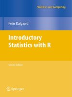
1.10 The registrar at State University keeps records of the number of credit hours students complete each semester.
The data he collects are summarized in the histogram. The class boundaries are 10 to less than 13, 13 to less than 16,
16 to less than 19, 19 to less than 22, and 22 to less than 25.

This content is available for free at />

CHAPTER 1 | SAMPLING AND DATA

Figure 1.4

What type of data does this graph show?

Qualitative Data Discussion

Below are tables comparing the number of part-time and full-time students at De Anza College and Foothill College
enrolled for the spring 2010 quarter. The tables display counts (frequencies) and percentages or proportions (relative
frequencies). The percent columns make comparing the same categories in the colleges easier. Displaying percentages along
with the numbers is often helpful, but it is particularly important when comparing sets of data that do not have the same
totals, such as the total enrollments for both colleges in this example. Notice how much larger the percentage for part-time
students at Foothill College is compared to De Anza College.

De Anza College

Foothill College

Number Percent

Number Percent

Full-time 9,200

40.9%

Full-time 4,059

28.6%

Part-time 13,296

59.1%

Part-time 10,124

71.4%

Total

100%

Total

100%

22,496

14,183

Table 1.2 Fall Term 2007 (Census day)

Tables are a good way of organizing and displaying data. But graphs can be even more helpful in understanding the data.
There are no strict rules concerning which graphs to use. Two graphs that are used to display qualitative data are pie charts
and bar graphs.
In a pie chart, categories of data are represented by wedges in a circle and are proportional in size to the percent of
individuals in each category.
In a bar graph, the length of the bar for each category is proportional to the number or percent of individuals in each
category. Bars may be vertical or horizontal.
A Pareto chart consists of bars that are sorted into order by category size (largest to smallest).
Look at Figure 1.5 and Figure 1.6 and determine which graph (pie or bar) you think displays the comparisons better.
It is a good idea to look at a variety of graphs to see which is the most helpful in displaying the data. We might make
different choices of what we think is the “best” graph depending on the data and the context. Our choice also depends on
what we are using the data for.

17

18

CHAPTER 1 | SAMPLING AND DATA

(a)

(b)

Figure 1.5

Figure 1.6

Percentages That Add to More (or Less) Than 100%
Sometimes percentages add up to be more than 100% (or less than 100%). In the graph, the percentages add to more than
100% because students can be in more than one category. A bar graph is appropriate to compare the relative size of the
categories. A pie chart cannot be used. It also could not be used if the percentages added to less than 100%.

Characteristic/Category

Percent

Full-Time Students

40.9%

Students who intend to transfer to a 4-year educational institution 48.6%
Students under age 25

61.0%

TOTAL

150.5%

Table 1.3 De Anza College Spring 2010

This content is available for free at />

CHAPTER 1 | SAMPLING AND DATA

Figure 1.7

Omitting Categories/Missing Data
The table displays Ethnicity of Students but is missing the "Other/Unknown" category. This category contains people who
did not feel they fit into any of the ethnicity categories or declined to respond. Notice that the frequencies do not add up to
the total number of students. In this situation, create a bar graph and not a pie chart.

Frequency

Percent

Asian

8,794

36.1%

Black

1,412

5.8%

Filipino

1,298

5.3%

Hispanic

4,180

17.1%

Native American 146

0.6%

Pacific Islander

236

1.0%

White

5,978

24.5%

TOTAL

22,044 out of 24,382 90.4% out of 100%

Table 1.4 Ethnicity of Students at De Anza College Fall
Term 2007 (Census Day)

Figure 1.8

19


20

CHAPTER 1 | SAMPLING AND DATA

The following graph is the same as the previous graph but the “Other/Unknown” percent (9.6%) has been included. The
“Other/Unknown” category is large compared to some of the other categories (Native American, 0.6%, Pacific Islander
1.0%). This is important to know when we think about what the data are telling us.
This particular bar graph in Figure 1.9 can be difficult to understand visually. The graph in Figure 1.10 is a Pareto chart.
The Pareto chart has the bars sorted from largest to smallest and is easier to read and interpret.

Figure 1.9 Bar Graph with Other/Unknown Category

Figure 1.10 Pareto Chart With Bars Sorted by Size

Pie Charts: No Missing Data
The following pie charts have the “Other/Unknown” category included (since the percentages must add to 100%). The

chart in Figure 1.11b is organized by the size of each wedge, which makes it a more visually informative graph than the
unsorted, alphabetical graph in Figure 1.11a.

This content is available for free at />

CHAPTER 1 | SAMPLING AND DATA

(a)

(b)

Figure 1.11

Sampling
Gathering information about an entire population often costs too much or is virtually impossible. Instead, we use a sample
of the population. A sample should have the same characteristics as the population it is representing. Most statisticians
use various methods of random sampling in an attempt to achieve this goal. This section will describe a few of the most
common methods. There are several different methods of random sampling. In each form of random sampling, each
member of a population initially has an equal chance of being selected for the sample. Each method has pros and cons. The
easiest method to describe is called a simple random sample. Any group of n individuals is equally likely to be chosen by
any other group of n individuals if the simple random sampling technique is used. In other words, each sample of the same
size has an equal chance of being selected. For example, suppose Lisa wants to form a four-person study group (herself
and three other people) from her pre-calculus class, which has 31 members not including Lisa. To choose a simple random
sample of size three from the other members of her class, Lisa could put all 31 names in a hat, shake the hat, close her
eyes, and pick out three names. A more technological way is for Lisa to first list the last names of the members of her class
together with a two-digit number, as in Table 1.5:

ID

Name

ID

Name

ID

Name

00

Anselmo

11

King

21

Roquero

01

Bautista

12

Legeny

22

Roth

02

Bayani

13

Lundquist 23

Rowell

03

Cheng

14

Macierz

Salangsang

04

Cuarismo

15

Motogawa 25

Slade

05

Cuningham 16

Okimoto

26

Stratcher

06

Fontecha

17

Patel

27

Tallai

07

Hong

18

Price

28

Tran

08

Hoobler

19

Quizon

29

Wai

09

Jiao

20

Reyes

30

Wood

10

Khan

24

Table 1.5 Class Roster

Lisa can use a table of random numbers (found in many statistics books and mathematical handbooks), a calculator, or
a computer to generate random numbers. For this example, suppose Lisa chooses to generate random numbers from a
calculator. The numbers generated are as follows:
0.94360; 0.99832; 0.14669; 0.51470; 0.40581; 0.73381; 0.04399

21


22

CHAPTER 1 | SAMPLING AND DATA

Lisa reads two-digit groups until she has chosen three class members (that is, she reads 0.94360 as the groups 94, 43, 36,
60). Each random number may only contribute one class member. If she needed to, Lisa could have generated more random
numbers.
The random numbers 0.94360 and 0.99832 do not contain appropriate two digit numbers. However the third random
number, 0.14669, contains 14 (the fourth random number also contains 14), the fifth random number contains 05, and the
seventh random number contains 04. The two-digit number 14 corresponds to Macierz, 05 corresponds to Cuningham, and
04 corresponds to Cuarismo. Besides herself, Lisa’s group will consist of Marcierz, Cuningham, and Cuarismo.

To generate random numbers:

• Press MATH.
• Arrow over to PRB.
• Press 5:randInt(. Enter 0, 30).
• Press ENTER for the first random number.
• Press ENTER two more times for the other 2 random numbers. If there is a repeat press ENTER again.
Note: randInt(0, 30, 3) will generate 3 random numbers.

Figure 1.12

Besides simple random sampling, there are other forms of sampling that involve a chance process for getting the sample.
Other well-known random sampling methods are the stratified sample, the cluster sample, and the systematic
sample.
To choose a stratified sample, divide the population into groups called strata and then take a proportionate number
from each stratum. For example, you could stratify (group) your college population by department and then choose a
proportionate simple random sample from each stratum (each department) to get a stratified random sample. To choose
a simple random sample from each department, number each member of the first department, number each member of
the second department, and do the same for the remaining departments. Then use simple random sampling to choose
proportionate numbers from the first department and do the same for each of the remaining departments. Those numbers
picked from the first department, picked from the second department, and so on represent the members who make up the
stratified sample.
To choose a cluster sample, divide the population into clusters (groups) and then randomly select some of the clusters.
All the members from these clusters are in the cluster sample. For example, if you randomly sample four departments
from your college population, the four departments make up the cluster sample. Divide your college faculty by department.
The departments are the clusters. Number each department, and then choose four different numbers using simple random
sampling. All members of the four departments with those numbers are the cluster sample.
To choose a systematic sample, randomly select a starting point and take every nth piece of data from a listing of the
population. For example, suppose you have to do a phone survey. Your phone book contains 20,000 residence listings. You
must choose 400 names for the sample. Number the population 1–20,000 and then use a simple random sample to pick a
number that represents the first name in the sample. Then choose every fiftieth name thereafter until you have a total of 400
names (you might have to go back to the beginning of your phone list). Systematic sampling is frequently chosen because

it is a simple method.
A type of sampling that is non-random is convenience sampling. Convenience sampling involves using results that are
readily available. For example, a computer software store conducts a marketing study by interviewing potential customers
This content is available for free at />

CHAPTER 1 | SAMPLING AND DATA

who happen to be in the store browsing through the available software. The results of convenience sampling may be very
good in some cases and highly biased (favor certain outcomes) in others.
Sampling data should be done very carefully. Collecting data carelessly can have devastating results. Surveys mailed to
households and then returned may be very biased (they may favor a certain group). It is better for the person conducting the
survey to select the sample respondents.
True random sampling is done with replacement. That is, once a member is picked, that member goes back into the
population and thus may be chosen more than once. However for practical reasons, in most populations, simple random
sampling is done without replacement. Surveys are typically done without replacement. That is, a member of the
population may be chosen only once. Most samples are taken from large populations and the sample tends to be small in
comparison to the population. Since this is the case, sampling without replacement is approximately the same as sampling
with replacement because the chance of picking the same individual more than once with replacement is very low.
In a college population of 10,000 people, suppose you want to pick a sample of 1,000 randomly for a survey. For any
particular sample of 1,000, if you are sampling with replacement,
• the chance of picking the first person is 1,000 out of 10,000 (0.1000);
• the chance of picking a different second person for this sample is 999 out of 10,000 (0.0999);
• the chance of picking the same person again is 1 out of 10,000 (very low).
If you are sampling without replacement,
• the chance of picking the first person for any particular sample is 1000 out of 10,000 (0.1000);
• the chance of picking a different second person is 999 out of 9,999 (0.0999);
• you do not replace the first person before picking the next person.
Compare the fractions 999/10,000 and 999/9,999. For accuracy, carry the decimal answers to four decimal places. To four
decimal places, these numbers are equivalent (0.0999).
Sampling without replacement instead of sampling with replacement becomes a mathematical issue only when the

population is small. For example, if the population is 25 people, the sample is ten, and you are sampling with replacement
for any particular sample, then the chance of picking the first person is ten out of 25, and the chance of picking a different
second person is nine out of 25 (you replace the first person).
If you sample without replacement, then the chance of picking the first person is ten out of 25, and then the chance of
picking the second person (who is different) is nine out of 24 (you do not replace the first person).
Compare the fractions 9/25 and 9/24. To four decimal places, 9/25 = 0.3600 and 9/24 = 0.3750. To four decimal places,
these numbers are not equivalent.
When you analyze data, it is important to be aware of sampling errors and nonsampling errors. The actual process of
sampling causes sampling errors. For example, the sample may not be large enough. Factors not related to the sampling
process cause nonsampling errors. A defective counting device can cause a nonsampling error.
In reality, a sample will never be exactly representative of the population so there will always be some sampling error. As a
rule, the larger the sample, the smaller the sampling error.
In statistics, a sampling bias is created when a sample is collected from a population and some members of the population
are not as likely to be chosen as others (remember, each member of the population should have an equally likely chance of
being chosen). When a sampling bias happens, there can be incorrect conclusions drawn about the population that is being
studied.

Example 1.11
A study is done to determine the average tuition that San Jose State undergraduate students pay per semester.
Each student in the following samples is asked how much tuition he or she paid for the Fall semester. What is the
type of sampling in each case?
a. A sample of 100 undergraduate San Jose State students is taken by organizing the students’ names by
classification (freshman, sophomore, junior, or senior), and then selecting 25 students from each.
b. A random number generator is used to select a student from the alphabetical listing of all undergraduate
students in the Fall semester. Starting with that student, every 50th student is chosen until 75 students are
included in the sample.
c. A completely random method is used to select 75 students. Each undergraduate student in the fall semester
has the same probability of being chosen at any stage of the sampling process.

23

24

CHAPTER 1 | SAMPLING AND DATA

d. The freshman, sophomore, junior, and senior years are numbered one, two, three, and four, respectively.
A random number generator is used to pick two of those years. All students in those two years are in the
sample.
e. An administrative assistant is asked to stand in front of the library one Wednesday and to ask the first 100
undergraduate students he encounters what they paid for tuition the Fall semester. Those 100 students are
the sample.
Solution 1.11
a. stratified; b. systematic; c. simple random; d. cluster; e. convenience

1.11 You are going to use the random number generator to generate different types of samples from the data.
This table displays six sets of quiz scores (each quiz counts 10 points) for an elementary statistics class.

#1

#2

#3

#4

#5

#6

5

7

10

9

8

3

10

5

9

8

7

6

9

10

8

6

7

9

9

10

10

9

8

9

7

8

9

5

7

4

9

9

9

10

8

7

7

7

10

9

8

8

8

8

9

10

8

8

9

7

8

7

7

8

8

8

10

9

8

7

Table 1.6

Instructions: Use the Random Number Generator to pick samples.
1. Create a stratified sample by column. Pick three quiz scores randomly from each column.
◦ Number each row one through ten.
◦ On your calculator, press Math and arrow over to PRB.
◦ For column 1, Press 5:randInt( and enter 1,10). Press ENTER. Record the number. Press ENTER 2 more
times (even the repeats). Record these numbers. Record the three quiz scores in column one that correspond
to these three numbers.
◦ Repeat for columns two through six.
◦ These 18 quiz scores are a stratified sample.
2. Create a cluster sample by picking two of the columns. Use the column numbers: one through six.
◦ Press MATH and arrow over to PRB.
◦ Press 5:randInt( and enter 1,6). Press ENTER. Record the number. Press ENTER and record that number.
◦ The two numbers are for two of the columns.
◦ The quiz scores (20 of them) in these 2 columns are the cluster sample.
3. Create a simple random sample of 15 quiz scores.
◦ Use the numbering one through 60.
◦ Press MATH. Arrow over to PRB. Press 5:randInt( and enter 1, 60).

This content is available for free at />

CHAPTER 1 | SAMPLING AND DATA

◦ Press ENTER 15 times and record the numbers.
◦ Record the quiz scores that correspond to these numbers.
◦ These 15 quiz scores are the systematic sample.
4. Create a systematic sample of 12 quiz scores.
◦ Use the numbering one through 60.
◦ Press MATH. Arrow over to PRB. Press 5:randInt( and enter 1, 60).

◦ Press ENTER. Record the number and the first quiz score. From that number, count ten quiz scores and
record that quiz score. Keep counting ten quiz scores and recording the quiz score until you have a sample
of 12 quiz scores. You may wrap around (go back to the beginning).

Example 1.12
Determine the type of sampling used (simple random, stratified, systematic, cluster, or convenience).
a. A soccer coach selects six players from a group of boys aged eight to ten, seven players from a group of
boys aged 11 to 12, and three players from a group of boys aged 13 to 14 to form a recreational soccer team.
b. A pollster interviews all human resource personnel in five different high tech companies.
c. A high school educational researcher interviews 50 high school female teachers and 50 high school male
teachers.
d. A medical researcher interviews every third cancer patient from a list of cancer patients at a local hospital.
e. A high school counselor uses a computer to generate 50 random numbers and then picks students whose
names correspond to the numbers.
f. A student interviews classmates in his algebra class to determine how many pairs of jeans a student owns,
on the average.
Solution 1.12
a. stratified; b. cluster; c. stratified; d. systematic; e. simple random; f.convenience

1.12 Determine the type of sampling used (simple random, stratified, systematic, cluster, or convenience).
A high school principal polls 50 freshmen, 50 sophomores, 50 juniors, and 50 seniors regarding policy changes for
after school activities.

If we were to examine two samples representing the same population, even if we used random sampling methods for the
samples, they would not be exactly the same. Just as there is variation in data, there is variation in samples. As you become
accustomed to sampling, the variability will begin to seem natural.

Example 1.13
Suppose ABC College has 10,000 part-time students (the population). We are interested in the average amount of
money a part-time student spends on books in the fall term. Asking all 10,000 students is an almost impossible

task.
Suppose we take two different samples.
First, we use convenience sampling and survey ten students from a first term organic chemistry class. Many of
these students are taking first term calculus in addition to the organic chemistry class. The amount of money they
spend on books is as follows:
$128; $87; $173; $116; $130; $204; $147; $189; $93; $153

25