The proper generalized decomposition for advanced numerical simulations ch33

Chapter 6
Numerical examples for linear analysis.
This Chapter presents numerical examples of several linear test problems. These
are used to validate the formulation of the linear ANDES elements that represents the “kernel” of the co-rotational formulation.

6.1

Patch tests.

The Patch Test has become a standard test for evaluation of new finite elements. Though neither a necessary or sufficient condition for convergence, it
has a strong following who considers the test “necessary” for an element to be
considered reliable. However, there is little disagreement about the tests value
as a debugging tool when an element is implemented in an actual finite element
code.
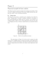
y

1

1
Figure 6.1.

x

Patch test for quadrilateral elements.

The patch shown on Figure 6.1 has been used to perform the patch
test for the new ANDES4 element by giving the boundary nodes displacements
according to a constant strain pattern. The patch test requires that the internal
nodes get displacements that satisfies this constant strain displacement mode
exactly.

1


Membrane tests.
u=x
v=y
u = y, v = x

∂u
=1
: Identically satisfied.
∂x
∂v
⇒ yy =
=1
: Identically satisfied.
∂y
∂u ∂v
⇒ γxy = (
+
) = 2 : Identically satisfied.
∂y
∂x
⇒

xx

=

Bending tests.

∂2w
=2
∂x2
∂2w
=
=2
∂y 2
∂2w
=2
=2
∂x∂y

w = x2

⇒ κxx =

:

Identically satisfied.

w = y2

⇒ κyy

:

Identically satisfied.

w = xy

⇒ κxy

:

Identically satisfied.

The membrane patch test for the ANDES4 element are satisfied regardless of
whether the higher order strain displacement matrix Bh or the deviatoric higher
¯ h is used for the higher order
order strain displacement matrix Bd = Bh − B
membrane stiffness according to equation (0.0.0) and (0.0.0).

6.2

Membrane problems.

6.2.1 Shear-loaded cantilever beam.
A shear loaded cantilever beam is defined according to Figure 8.1. This Figure
also shows the 16 × 4 regular and irregular element meshes.
P=40

12

48

Figure 6.2.

Cantilever under end shear. E = 30000 ν = 0.25

2

The test has been run using a totally clamped boundary at the fixed
end, and the applied nodal forces on the end cross-section are consistent lumping
of a shear load with parabolic variation in the y-direction.
The comparison value is the tip deflection of 0.35583 at the end of the
beam. This number is the exact solution of the two-dimensional plane stress as
given in [28] . The numerical results have been scaled so that the analytical
displacement of 0.35583 corresponds to 100 in Table 6.1. Table 6.1 also includes
numerical results for the quatrilateral FFQ and the triangular FFT as described
by Nyg˚
ard in [47].

Table 6.1. Tip deflection of cantilever beam.
Element

CST
QSHELL3
QSHELL4

x×y -subdivisions
4×1
8×2
16×4 32×8
Regular element mesh
25.48
111.78
97.72

55.24

101.18
98.86

82.66
100.03
99.54

64×16

94.96
99.97
99.87

98.71
100.01
100.00

94.27
99.87
99.90

98.41
99.97
100.01

Irregular element mesh
CST
QSHELL3
QSHELL4

27.86
98.16
103.93

55.84
100.12
98.60

81.47
99.66
99.45

Table 6.1 shows very similar convergence rates for the QSHELL3 and
QSHELL4 element compared to Nyg˚
ards FFT and FFQ element. However, the
ANDES elements tend to be more flexible for very coarse meshes.

6.3

Bending problems.

6.3.1 Centrally loaded square plate.
A square plate subjected to a central load of P = 40.0. The test has been run
with both simply supported and fully clamped boundary conditions.
Plate dimensions are 100.0 × 100.0 with thickness t = 2.0 and material
properties E = 1500.0 and ν = 0.2 . Due to symmetry only a quarter of the
plate have been modeled.

3

thickness h
L

P/4

symm

d
pe

clamped
L

Figure 6.3.

sy

m
m

m

cla

4×4 quarter model of centrally loaded square plate.

Table 6.2. Central deflection of square plate with clamped
boundary. Displacement 2.1552 is scaled to 100.00 .
Element

type

1×1

Mesh over quarter plate
2×2
4×4
8×8 16×16

32×32

Regular mesh.

6.4

BCIZ-SQ
ANDES3
ANDES4

88.223 102.71 101.18 100.37
92.798 103.75 101.57 100.50
88.944 100.07 100.18 100.07
Irregular mesh.

100.10
100.15
100.02

100.02
100.04

100.00

BCIZ-SQ
ANDES3
ANDES4

88.223 99.805 101.27 99.781
92.798 102.48 102.38 100.40
88.944 99.793 101.71 100.19

99.983
100.23
100.14

99.938
100.02
100.02

Shell problems.

6.4.1 Pinched cylinder problem.
An open cylinder is subjected to two diametrically opposite point loads. Due to
symmetry only 1/8 of the problem is modeled. The geometry of the 1/8 model
is shown in Figure 6.4.
The mesh has been given an increasing distortion angle θ. As θ increases
the four node elements are no longer flat elements. This induced warping gives
different results for the projected and unprojected versions of the ANDES4 element. The ANDES3 element is invariant under projection because the element
always possesses the correct rigid body modes.
The improvement with the projected stiffness matrix for the ANDES4
element is dramatic. This example displays the importance of correct rigid body

modes, as well as showing the robustness of the stiffness projection procedure.
4


P

y

R = 4.953
L = 5.175
h = 0.094
E = 10.5e+6
ν = 0.3125

θ

R
x
-hL
z

Figure 6.4.

Pinched cylinder problem.

Table 6.3. Vertical displacement under load for pinched
cylinder. Displacement 4.5301×10−3 is scaled to 100.00.
Element
type
ANDES3

ANDES3
ANDES4
ANDES4

◦

θ=0
Unproj
Proj
Unproj
Proj

99.578
99.578
99.430
99.430

Distortion angle
θ = 10◦ θ = 20◦ θ = 30◦
99.136
99.136
30.594
99.334

98.737
98.737
12.652
99.255

98.296

98.296
9.381
99.125

θ = 40◦
97.608
97.608
7.960
98.789

6.4.2 Pinched hemisphere problem.
A hemispherical shell is subjected to two pairs of diametrically opposite loads
along the x and y axis respectively. Due to symmetry only a 1/4 model is used
according to Figure 6.5.
This problem is often modelled with a hole at the top of the hemisphere.
This allows using a mesh of strictly flat quadrilateral elements, which makes
the test much less demanding for quadrilateral elements. One has chosen to
model the hemisphere without a hole since this gives warped elements for the
quadrilateral element meshes, and thus poses a much more severe test for those
elements.
For the triangular ANDES3 two discretizations are used. Mesh 1 in
Table 6.4 refers to a mesh where two triangular elements join at the loaded
nodes, whereas Mesh 2 has one element attached to the loaded nodes.

5


Z
R = 10.0
h = 0.04

fixed

E = 6.825x107
ν = 0.3
F = 1.0

sy
sym

m

F
Y
F

free

X

Figure 6.5.

Pinched hemisphere problem.

Table 6.4. Displacements under loads for pinched hemisphere. Displacement 9.1898×10−2 is scaled to 100.00.
Element
type
ANDES3
ANDES3
ANDES4

ANDES4

2
Mesh 1
Mesh 2
Unproj
Proj

Elements per side
4
8
12
16

20

0.18
2.59 25.30 61.44 83.23
92.52
0.42
4.07 31.91 68.23 86.85
94.23
13.57
6.13 12.85 19.49 25.17
30.18
67.55 23.73 85.53 97.24 99.39 100.00

This test again shows the dramatic improvement of the performance of
the ANDES4 element when the stiffness projection is used.

6


Chapter 7
Numerical examples for linearized buckling analysis.
7.1

Buckling analysis of square plate compressed in one
direction.

The buckling of a square plate subjected to in-plane uniaxial compression is
considered. The geometry and material constants of the plate are given in
Figure 7.1. The plate is simply supported along all edges with the in-plane
deformations being unconstrained.

y
L
Nx
sym

sym
-tNx

L = 508 mm
t = 3.175 mm

L

2
E = 2.062e5 N/mm

v = 0.3

Figure 7.1.

x

Square plate subjected to uniaxial compression.

The plate is compressed in its middle plane by a uniform load Nx along
the edges x = 0 and x = L. Timoshenko [63] gives the analytical critical value
of the compressive force per unit length as
(Nx )cr =

π2 D
1 2
(m
+
)
L2
m

where

D=

Et3
.
12(1 − ν 2 )

(7.1.1)

where L is plate side length, t is the plate thickness, ν is the Poisson’s ratio and
m is the number of half-waves in the compressive direction. The buckling modes
are associated with odd values of m.
The geometric stiffness is based on the incremental solution at a load
level of 1% of the critical load level. The results from the numerical analysis is
tabulated in Table 7.2 and compared to results obtained by Bjærum [17] with
7


the QSEL and FFQC elements. The QSEL and FFQC elements performs better
than ANDES3 and ANDES4 for the higher order buckling modes. This is due
to the “tuned” higher order geometric stiffness matrix used for those elements.
However the geometric stiffness matrices used for the QSEL and FFQC element
do not give a consistent tangent stiffness for nonlinear continuation analysis.

Table 7.1. Numerical results of square plate subjected to
compression, normalized by the analytical solution of the
first mode (m = 1).
Element
Type

Analytical
Solution

Mesh used for quarter of plate
4 × 4 8 × 8 16 × 16 32 × 32

ANDES3

m = 1:
m = 3:
m = 5:
m = 1:
m = 3:
m = 5:
m = 1:
m = 3:
m = 5:
m = 1:
m = 3:
m = 5:

1.008
3.070
8.342
1.043
3.278
10.11
1.010
3.032
8.751
0.973
2.673
6.750

ANDES4

QSEL

FFQC

1.000
2.778
6.760
1.000
2.778
6.760
1.000
2.778
6.760
1.000
2.778
6.760

8

1.002
2.854
7.270
1.011
2.898
7.522
1.002
2.840
7.265
0.993
2.745
6.694

1.000
2.797
6.893
1.002
2.808
6.950
1.001
2.793
6.884
0.998
2.769
6.738

1.000
2.783
6.798
1.001
2.786
6.815
1.000
2.782
6.791
1.000
2.778
6.754


Figure 7.2.

7.2

Buckling modes for m = 1, 3 and 5 according to equation (7.1.1)
for square plate subjected to uniaxial compression.

Buckling analysis of shear loaded square plate.

A simply supported square plate with geometry and material constants given in
Figure 7.3 is subjected to shear loads uniformly applied along the edges. The
out-of-plane displacements and rotations are constrained whereas the in-plane
rotations and translations along the boundaries are left free.
The critical shear force associated with the first buckling mode is give
analytically by Timoshenko [63] as
(Nxy )cr = 9.34

π2 D
L2

where

9

D=

Et3
.
12(1 − ν 2 )

(7.2.1)

y

L

Nxy

L = 1000 mm
t = 12.5 mm

Nxy

L

2
E = 6.4e3 N/mm
v = 0.3
Nxy= 105.5 N/mm

Figure 7.3.

x

Square plate subjected to shear load.

Table 7.2. Numerical results of square plate subjected to shear, normalized by the analytical soluN
.
tion (Nxy )cr = 105.5 mm
Element
Type
ANDES3 m = 1:

m = 2:
m = 3:
ANDES4 m = 1:
m = 2:
m = 3:
QSEL
m = 1:
m = 2:
m = 3:
FFQC
m = 1:
m = 2:
m = 3:

4×4
1.446
2.174
8.631
2.175
3.079
1.387
2.096
207.3
0.781
1.060
2.073

Mesh used for the plate
8 × 8 16 × 16 32 × 32

64 × 64

1.145
1.293
2.974
1.297
1.528
4.300
1.065
1.385
3.582
0.908
1.144
2.301

0.993
1.233
2.642
0.994
1.233
2.643

1.057
1.240
2.709
1.088
1.298
3.013
1.008
1.268

2.840
0.967
1.206
2.518

1.013
1.238
2.675
1.022
1.250
2.739
0.997
1.242
2.691
0.987
1.227
2.614

This problem again shows that the higher order geometric stiffness matrix for the QSEL and FFQC element outperforms the consistent geometric
stiffness matrix of the ANDES elements for linearized buckling analysis. The
ANDES3 element performs better than the ANDES4 element simply because
10


meshes of N × N elements contains twice as many ANDES3 elements as ANDES4 elements since two triangles are required to fill one quadrilateral. This
gives a “finer” discretization with respect to the rigid body displacements and
thus a better global geometric stiffness matrix.

11

Figure 7.4.

First three buckling modes for shear loaded square plate.

12


Chapter 8
Numerical examples for nonlinear analysis.
8.1

Smooth path following problems.

8.1.1 Cantilever beam subjected to end moment.
The cantilever in Figure 6.2 is used to demonstrate the large rotation and large
displacement capabilities. The problem is usually formulated so that bending
about one of the global axes takes place. The cantilever here is oriented arbitrarily in space so that the example becomes more demanding as regards the
treatment of finite rotations as non-vectorial quantities. The position of the
cantilever is defined by the auxiliary coordinate system
 

 
¯
6 −2 −3  x 
x
1
y¯ =  3 6
2  y ,
(8.1.1)

  7
 
z¯
2 −3 6
z
and letting one side of the cantilever follow the x
¯-axis. This auxiliary system
is used for modeling purposes only. The actual computations take place in the
global (x, y, z)-system.
The exact solution is obtained from Bernoulli-Euler beam theory, and
gives the deflected shape of the beam as a circle with radius
R=

EI
.
My¯

(8.1.2)

This gives the tip deflections as
w
¯
EI
M − y¯L
=
(1 − cos
)
L
My¯L
EI

and

v¯
EI
M − y¯L
=−
sin
L
My¯L
EI

(8.1.3)

where w
¯ and v¯ are the deflections in the x
¯- and z¯- directions.
The problem was solved using load control with the incremental load
ML
steps ∆My¯ = 2π
40 EI , thus requiring 40 steps to bend the beam into a full
circle. This small load step was required for the triangular element due to the
large unbalanced membrane forces that are introduced during the iterations.
The triangular element does not give symmetry about the center line of the
cantilever, and thus converges more slowly than a comparable four node element,

13


L = 10.0 m

b = 1.0 m
h = 0.1 m
E = 1.2e3 MPa
ν = 0.0

b

L

Figure 8.1.

Cantilever oriented arbitrarily in space
subjected to end moment.

as described by Nyg˚
ard [47] . For the ANDES4 element the beam was bent into
a full circle using 10 load steps.
Table 8.1 gives convergence rates and number of iterations for the cantilever modeled with 20 ANDES3 elements. The label “Fit type” refers to the
G matrix used for fitting the shadow element, with 1, 2 and 3 signifying side 12
alignment, least square fit of side edge angular errors and CST rotation, respectively. “1 diag” means that side 12 is directed along the diagonal of a rectangle
assembly of two elements whereas “1 edge” means that side 12 is directed along
the beam axis. Table 8.1 illustrates two points: Side 12 alignment is not orientation invariant since it doubles the number of iterations of the “1 diag” mesh
compared to “1 edge”. Also, the applied load is a moment load, which gives
a geometric stiffness that does not go towards symmetry as equilibrium is approached. The symmetrized stiffness will thus give poor convergence compared
to the nonsymmetric tangent stiffness.

14


Table 8.1. Iterations for the first 10 steps.

Symmetric stiffness
Fit type
1 edge.
1 diag.
2
3

Num. of iterations
4
9
5
4

4
9
5
4

Fit type
1 edge.
1 diag.
2
3

5 5 6 7 8
9 9 9 10 11
5 6 6 7 8
5 5 6 7 8
Non-symmetric stiffness

Conv.
8 8 9 L
9 10 10 L
8 8 8 L
8 8 9 L

Num. of iterations
4
8
5
4

4
8
5
4

4
8
5
4

4
9
5
4

4
8
5

4

4
8
5
4

4
9
5
4

Conv.
4
9
5
4

4
9
5
4

4
9
5
4

1.0
v : 2 x 19 nodes

u : 2 x 19 nodes

Load

0.8

0.6

0.4

0.2

0
0

2

Figure 8.2.

4

6
8
Displacement

10

12

Tip displacements of the cantilever beam

subjected to end moment.

8.1.2 Hinged cylindrical shell under concentrated load.

15

Q
Q
Q
Q


B
P
L
A
-hL

R = 2540 mm
L = 254 mm
h = 6.35 mm or 12.7 mm
E = 3.10275 N/mm2

R
θ

v = 0.3
θ = 0.2 rad

Figure 8.3.

Geometry and material properties for
hinged cylindrical shell.

The hinged cylindrical shell subjected to concentrated load is a common test
case for geometrical nonlinearities. Nyg˚
ard [47] performs an extensive comparison with other elements. Bjærum [17] gives a thorough comparison of
different path-following algorithms for this example. The thinner shell of thickness h = 6.35mm has a dramatic snap-back behavior well suited for verifying
path following capabilities of the solution algorithm.
One quarter of the shell has been modeled using 8 × 8 rectangular units
of two three node elements. The actual equilibrium path shown in Figures 8.4
and 8.5 agrees well with results obtained by Nyg˚
ard [47].
The arc-length algorithm did not evidence convergence difficulties. With
the thin shell the path has been followed using 26 steps and convergence was
obtained within 5 iterations even at the snap-back section of the equilibrium
path.

16


4.0
3.5

Point A
Point B

3.0

Load

2.5
2.0
1.5
1.0
0.5
0
0

5

Figure 8.4.

10

15
20
Z-displacement

25

30

Vertical deflection at points A and B
for hinged cylindrical panel with t = 12.7mm.

1.0
Point A
Point B

0.8

Load

0.6
0.4
0.2
0
-0.2
-0.4
-5

Figure 8.5.

0

5

10
15
Z-displacement

20

25

Vertical deflection at points A and B
for hinged cylindrical panel with t = 6.35mm.

17

30


8.1.3 Pinching of a clamped cylinder.
A cantilevered cylinder is subjected to two diametrically opposite forces of magnitude F at the open end. Due to symmetry only a quarter of the structure is
modelled. The problem has been studied by Stander et al. [60] and Parisch
[48] using uniform element meshes. Mathisen, Kvamsdal and Okstad [43] have
studied this problem using adaptive mesh techniques. The present analysis was
performed using displacement control of the loaded point with 16 equal step up
to a total displacement of 1.6 times the radius of the cylinder.

cla

F/2

m

d

pe
m

sy

e

fre

-h-

m

sy

L

R = 1.016
L = 3.048
h = 0.03
E = 2.0685e+7
ν = 0.3

R

Figure 8.6.

Geometry and material properties for the
pinched cylinder problem.

This example shows that the ANDES4 element is better than the ANDES3 element with respect to membrane strain gradients. A mesh of 16 × 16
ANDES3 elements diverges before the analysis is completed, whereas a mesh
of 16×16 ANDES4 elements is sufficient to complete the analysis as shown in
Figure 8.7. The results in Figure 8.7 shows good agreement with the results obtained by Stander et al. [60] and Parish [48], both of whom used quadrilateral
elements.
8.1.4 Stretched cylinder with free ends.
A open cylinder with free ends are subjected to two diametrically opposite forces
at the halflength. Geometric data for the cylinder are given in Figure 8.9. This
problem was first discussed by Gruttman et al. [32], and later by Peri´c and
Owen [50]. Figure 8.10 shows the results of the present analysis with a mesh of

8×16 ANDES4 elements compared with Peri´c and Owens analysis using a mesh
of 10×20 elements. The displacement of the loaded point agrees well with the
results reported in [50] .

18


1000
ANDES4 16x16
ANDES3 16x16
ANDES3 24x24
Stander et al. 32x32
Parisch 16x16

Load

800

600

400

200

0
0

Figure 8.7.

Figure 8.8.

0.5

1.0
Displacement

1.5

Vertical displacement at loading point for the
pinched cylinder problem.

Deformed finite element mesh at various loads.

19


F/4
sym

sy

L = 10.35
R = 4.935
h = 0.094
E = 10.5e+6
ν = 0.3125
F = 50.0

m

fre
e

-hm

sy

L

R

Figure 8.9.

Geometry and material properties for the
stretch cylinder problem.

700
Horizontal center displ.
Horizontal edge displ.
Vertical displ. at load
Peric & Owen 10x20 mesh

600

Load

500
400
300
200

100
0
0

0.5

1.0

Figure 8.10.

1.5

2.0
2.5
Displacement

3.0

3.5

Load displacement curves for the
stretched cylinder problem.

20

4.0

4.5

Figure 8.11.

Deformed finite element mesh at various loads.

21


8.2

Path-following problems with bifurcation.

8.2.1 Post-buckling analysis of square plate compressed in one direction.
The geometry and material properties of the square plate are presented in Figure
7.1. The applied load is normalized with respect to the analytical buckling load
for this problem given in equation (7.1.1) .
The post-buckling analysis is performed in order to evaluate the stiffness
properties of the plate after bifurcation is encountered. One has used a 8 × 8
mesh of ANDES4 elements over the quarter model. This mesh gave about 1%
error in determining the linearized buckling load.

2.0

Normalized load

1.5

1.0

Bifurcation analysis
1% imperfection

10% imperfection
50% imperfection

0.5

0
-1

Figure 8.12.

0

1

2

3
4
5
6
z-displacement in mm

7

8

9

Out of plane displacement at plate center for square plate
subjected to compression.

As seen in the load displacements curves in Figure 8.12 the structure
shows a stable post-buckling response where it can withstand increased load
after bifurcation. Figure 8.12 also shows the response of the plate with various
geometric imperfection levels. The buckling mode of the structure has been
scaled so that the largest out of plane imperfection is equal to 1%, 10% and 50%
of the plate thickness.

22


8.2.2 Post-buckling analysis of shear loaded square plate.
The geometry and material properties of the square plate are described in Figure
7.3. The applied load is normalized with respect to the analytical buckling load
N
Nxy cr = 105.5 mm
.
A 16 × 16 mesh of ANDES3 elements over the quarter model is used.
This mesh gave about 5% error in determining the linearized buckling load. It
should be noted that the shear loaded plate has traditionally been a difficult
problem for triangular elements.

2.0

Normalized load

1.5

1.0

0.5

Bifurcation analysis
1% imperfection
10% imperfection

0
0

Figure 8.13.

5

10

15
20
25
z-displacement in mm

30

35

40

Out of plane displacement at plate center for square plate
subjected to compression.

As seen in the load displacements curves in Figure 8.13 the structure

shows a stable post-buckling response where it can withstand increased load
after bifurcation. Figure 8.13 also shows the response of the plate with various
geometric imperfection levels. The buckling mode of the structure has been
scaled so that the largest out of plane imperfection is equal to 1% and 10% of
the plate thickness.

23


8.2.3 Buckling of a deep circular arch.
This problem of snap-through of a deep circular arch has been investigated by
Huddlestone [37] . The asymmetric displacement path has been studied by Simons et al. [59] and Feenstra and Schellekens [23] using a small geometric
imperfection to induce the buckling mode. Bjærum [17] analyzed the problem using branch switching to follow the secondary path. The present analysis
follows Bjærum’s in that no imperfection is used, and the branch switching
algorithm has been used to traverse the bifurcation and continuing along the
secondary path.
The dimensions of the arch are given in Figure 8.14. The arch has hinged
boundary conditions at both ends and is modelled using 20 quadrilateral shell
elements with the z displacements constrained.

P

h

H

E = 2.1e+5 N/mm2
ν =0

R

z
L/2

R = 1000 mm
L = 1600 mm
H = 400 mm
h = 10 mm

L/2

x

Figure 8.14.

Geometry and material properties for the deep
circular arch.

Figure 8.15 shows the response of the structure for the primary path, and
the secondary path obtained by doing a branch switching at the first bifurcation
R2
R2
point at PEI
= 13.2. Bjærum reports a bifurcation point at PEI
= 12.0, and
from his plot of the secondary path one can see that the load then jumps to
approximately 13.0. Such a gap between detected and converged bifurcation
points as reported by Bjærum can indicate an inconsistent tangent stiffness
matrix. The deflections of these paths are also illustrated in Figure 8.16
The problem displays some puzzling behaviour. For instance, the primary path appears not to intersect with the secondary path. The primary path
keeps doing spiraling motions for the vertical displacement versus load as plotted in Figure 8.17. For each spiraling motion another wavelike deformation is

24


20
15

Load

10
5
0
Vertical disp. secondary path
Vertical disp. primary path
Horizontal disp. secondary path

-5
-10
-100

0

100

200
300
400
Displacement

500

600

700

Figure 8.15.

Displacements for the primary and secondary paths.

Figure 8.16.

Deformations for the secondary and primary paths.

fed into the arch as shown in Figure 8.18. The fact that the primary and secondary path do not intersect can be discerned from the fact that the primary
path never achieves the same vertical deflection for the midpoint of the arch as
the secondary path.
The secondary path keeps doing figure-of-eight like motions for the midpoint of the arch. The branch switching algorithm does not pick up a new bifurcation point at the bottom point of the secondary path as would be expected.
25