The proper generalized decomposition for advanced numerical simulations ch32

Chapter 5
Quadrilateral Shell Elements.
Flat quadrilateral shell elements have use limitations even in linear analysis,
since a mesh that consists of strictly flat elements may be impossibly to construct
over a doubly-curved shell surface. For large deflection nonlinear analysis this
deficiency becomes more pronounced. Even if the initial mesh satisfies the flat
element restriction, the deformations can become so large that warping of the
elements can be significant. Finding ways of handling warped element geometries
is thus of fundamental importance for quadrilateral shell elements.
The current research initially set out to develop a non-flat quadrilateral
element that was able to satisfy self-equilibrium in a warped configuration. This
proved to be difficult. Finding a basic stiffness Kb = A1 LCLT that maintained
self equilibrium was especially troublesome. To achieve this goal one must have
the lumped node forces from a constant stress state f = Lσ to be in self equilibrium. Two questions arise at this point: What is a constant stress state for a
warped shell element? Is a constant stress state for a warped surface an equilibrium state for arbitrary element shapes? These are key questions that remain
to be answered in order to develop satisfactory FF and ANDES elements for
such element geometries. It follows that those formulations have to be further
extended for developing warped shell elements. The construction of the basic
stiffness matrix needs special attention because the Individual Element Test is
not clearly defined for curved or warped element geometries.
Restoring equilibrium in the warped element geometry can be done a
posteriori for elements developed with reference to the flat projected “footprint”
by using a projector matrix. This is the approach that has been chosen for the
current quadrilateral element. It allows independent development of the membrane and bending components since these two stiffness contributions decouple,
which greatly simplifies the development of the element. Both linear and nonlinear projectors have been developed for the quadrilateral element. Both versions
give identical results for linear static problems, but the linear projector is recommended for linear finite element codes because its formulation is much simpler
than that of the nonlinear projector.

1

5.1

Geometric definitions for a quadrilateral element.

This section describes geometric relationships for a quadrilateral element. The
development covers both warped geometry and the flat “best fit” element obtained by setting the z coordinate for each node equal to zero. The flat projection relationships are later used for the development of the membrane and
bending stiffness of the shell element. The non-flat relationships are needed for
the development of the nonlinear projector for quadrilaterals.
A vector r to a point on a nonflat quadrilateral element can be parametrized
with respect to the natural coordinates ξ and η as
  
 
N 0 0 x
x
r(ξ, η) = y =  0 N 0  y ,
(5.1.1)
 
 
z
0 0 N
z
where

 
x

 1

x2
x=

,

 x3 

x4

 
y1

 

y2
y=
,

 y3 

y4

 
z1

 

z2
z=
,

 z3 


z4

(5.1.2)

and xi , yi and zi denote the global coordinates of node i. Row vector N contains
the “usual” bi-linear isoparametric interpolation for a quadrilateral [00]. These
functions and their partial derivatives with respect to ξ and η are
1
[ (1 − ξ)(1 − η) (1 + ξ)(1 − η) (1 + ξ)(1 + η)
4
1
N,ξ = [ −(1 − η)
(1 − η)
(1 + η) −(1 + η) ] ,
4
1
N,η = [ −(1 − ξ) −(1 + ξ)
(1 + ξ)
(1 − ξ) ] .
4
N =

(1 − ξ)(1 + η) ] ,

(5.1.3)
Using these geometric relations the variation of the position vector r can be
written as
   ∂x dξ + ∂x dη   ∂x ∂x 

∂η

∂ξ
∂η
 dx  
 ∂ξ

 ∂y ∂y  dξ
∂y
∂y
dy = ∂ξ dξ + ∂η dη =  ∂ξ ∂η 
dη
  
 ∂z dξ + ∂z dη 

∂z
∂z
dz
∂ξ
∂η
∂ξ
∂η
(5.1.4)


N,ξ x N,η x
dξ
dξ
= [ gξ gη ]
=  N,ξ y N,η y 
dη
dη

N,ξ z N,η z
or
dr = Jdξ .
2


The Jacobian J introduced above is also used for computing partial derivatives
with respect to the natural coordinates ξ and η:
∂(·)
∂ξ
∂(·)
∂η

=
=

∂(·)
∂x
∂(·)
∂x

∂x
∂ξ
∂x
∂η

N,ξ x
N,η x

or

+
+

∂(·)
∂y
∂(·)
∂y

∂y
∂ξ
∂y
∂η

=

∂x
∂ξ
∂x
∂η

∂y
∂ξ
∂y
∂η

∂(·)
∂x
∂(·)
∂y

∂(·)
∂x
∂(·)
∂y

N,ξ y
N,η y

∂(·)
∂(·)
= JT
.
∂ξ
∂x

(5.1.5)

(5.1.6)

It should be noted that only the x and y components are included in the above
relationship for the partial derivatives. This is a consequence of assuming that
the element represents a best fit of the warped quadrilateral in the (x, y)-plane.
If the z-coordinate is neglected the relationship between (x, y) and (ξ, η)
is isoparametric and the inverse relation can be formed as
∂(·)
∂x
∂(·)
∂y

−T
Jxξ
=
−T
Jyξ

−T
Jxη
−T
Jyη

∂(·)
∂ξ
∂(·)
∂η

.

(5.1.7)

5.1.1 Geometric quantities for a flat quadrilateral element.
By defining lij to be length of side edge ij one obtains
lij =

2 .
x2ji + yji

(5.1.8)

The unit vector sij along side ij and the outward normal vector nij of side ij

can then be defined as





 

ni x   −si y 
xji 
 si x 


1
sij = si y =
yji
si x . (5.1.9)
and
nij = ni y =


 lij 

 

0
0
0
0

3


5.2

The quadrilateral membrane element.

Nyg˚
ard [00] developed a 4-node membrane element with drilling degrees of
freedom based on the Free Formulation, which is called the FFQ element. The
element has given accurate results for plane membrane problems. Unfortunately,
the element is computationally expensive because the formation of each element
stiffness requires the numerical inversion of a 12 × 12 matrix. The goal of the
present development is to construct a 4-node membrane element with the same
freedom configuration and similar accuracy as the FFQ, but that avoids those
expensive matrix inversion.
Recall that element stiffness of the ANDES element is the sum of the
basic and higher order contributions:
K = Kb + K h =

1
LCLT +
A

BTh CBh dA .

(5.2.1)

A

These matrices are now developed for the membrane component.
5.2.1 Basic stiffness.
The basic stiffness for the membrane element is developed by lumping the constant stress state over side edges to consistent nodal forces at the neighboring
nodes according to a boundary displacement field. When the boundary displacement field is defined so that interelement compatibility is satisfied, pairwise cancelation of nodal forces for a constant stress state is assured, and thus
satisfaction of the Individual Element Test [00]. In turn, satisfaction of the Individual Element Test ensures that the conventional multi-element Patch Test
is passed.
A very successful lumping scheme for membrane stresses was first introduced by Bergan and Felippa [00] in the paper describing the triangular
membrane FF element with drilling degrees of freedoms. This procedure has
since been used by Nyg˚
ard [00] and Militello [00].
The presentation here rewrites the lumping matrix, in terms of nodal
submatrices. The expressions of the lumping matrix thus becomes valid for
elements of arbitrary number of corner nodes.
It is convenient to order the visible degrees of freedom as translations
along x, y and drilling rotation about z-axis for each node. This gives the
lumping of the constant stress σ state to nodal forces f as


 σxx 
f = Lσ
where
σ = σyy ,
(5.2.2)


τxy

4




L1
L 
L= 2
L3
L4

 
f1


 
f2
and f =


 f3 
f4

where



 fx i 
.
fy
fi =
 i 

mz i

(5.2.3)

By using the Hermitian beam shape function for a side edge one obtains a boundary displacement field that is compatible between adjacent elements because the
displacements along an edge are only functions of the end nodes freedoms. This
again gives a lumping matrix L where each nodal contribution Lj is only a
function of its adjoining side edges ij and jk:


yki
1
Lj = 
0
2 α 2
2
6 (yij − ykj )

0
−xki
α
2
2
6 (xij − xkj )


−xki
.
yki
α

3 (xkj ykj − xij yij )

(5.2.4)

The nodal indices (i, j, k, l) for a four node element undergo cyclic permutations
of (1, 2, 3, 4) in the equation above. Factor α represents a scaling of the contributions of the drilling freedom to the normal boundary displacements; see [00]
for details.
5.2.2 Higher order stiffness.
To construct Kh a set of higher order degrees of freedoms that vanish for rigid
body and constant strain states is constructed.
Higher order degrees of freedom.
The 12 visible nodal degrees of freedom vx , vy and θ for each node are ordered
in an element displacement vector v as
 
 vx 
v = vy ,
 
θ

where

vTx = [ vx1

vx2

vx3

vx4 ] ,

vTy = [ vy1

vy2

vy3

vy4 ] ,

θT = [ θ1

θ2

θ3

(5.2.5)

θ4 ] .

The correct rank of the element stiffness matrix for the quadrilateral membrane
element is 9, coming from 12 degrees of freedom minus 3 rigid body modes. The
basic stiffness gives is rank 3 from the 3 constant strain modes. The higher order
stiffness must therefore be a rank 6 matrix. This can be conveniently achieved
by introducing 6 higher order “intrinsic” degrees of freedom, which are collected
˜ defined below.
in a vector v
Experience from the 3-node ANDES membrane element with drilling
degrees of freedom [00] and the 4-node ANDES tetrahedron solid element with

5

˜
rotational degrees of freedom [00], suggests using the hierarchical rotations θ
as higher order degrees of freedom:
˜ = θ − θ0 ,
θ

θT0 = [ θ0

θ0

θ0

θ0 ] ,

(5.2.6)

where the subtracted θ0 represents the overall or mean rotation of the element,
associated with rigid body and constant strain rotation motions. Furthermore,
splitting the hierarchical rotations into their mean and deviatoric parts as
¯ T = [ θ¯ θ¯ θ¯ θ¯ ] ,
θ

˜=θ
¯+θ,
θ

(5.2.7)

has the advantage of singling out the often troublesome “drilling mode”, or
“torsional mode”, where all the drilling node rotations take the same value with

all the other degrees of freedom being zero.
Unfortunately, the hierarchical rotations give only 4 higher order degrees
of freedom and at most a rank 4 update of the stiffness matrix. Two more higher
order degrees of freedom must be found. The element has 8 translational degrees
of freedom represented by vx and vy . The 3 rigid body and 3 constant strain
modes can all be described by the translational degrees of freedom. There are
still 2 higher order modes which can be described by the translational degrees
of freedom. These two modes must be recognized so as to associate two higher
order degrees of freedom with them. The amplitudes of the six higher order
degrees of freedom are then represented as
˜ T = [ θ1
v

θ2

θ3

θ4

θ¯ α1

α2 ] ,

(5.2.8)

where α1 and α2 are associated with the two higher order translational modes.
Although 7 degrees of freedom appear in this vector, the hierarchical rotation
constraint
4

θi = 0
i=1

reduces (5.2.8) effectively to six independent components.

6

(5.2.9)


Higher order rotational degrees of freedom.
θ0 is evaluated as the rotation of the bi-linear quadrilateral computed at the
element center given by (ξ = 0, η = 0), and is function of the translational
degrees of freedom only:
θ0 =

1 ∂v
∂u
1
(
−
) = [ −N,y
2 ∂x ∂y
2

vx
vy

N,x ]

.

(5.2.10)

By using the partial derivative expressions in equation (5.1.7) one obtains the
expressions for the rigid body and constant strain rotation as
1
[ x24 x31 x42 x13 ] ,
16|J|
1
−T
−T
[ y24 y31 y42 y13 ] ,
= −(Jxξ
N,ξ + Jxη
N,η ) =
16|J|

−T
−T
−N,y = −(Jyξ
N,ξ + Jyη
N,η ) =

N,x

(5.2.11)

where
|J| =

1
((x1 y2 − x2 y1 ) + (x2 y3 − x3 y2 ) + (x3 y4 − x4 y3 ) + (x4 y1 − x1 y4 )). (5.2.12)
8

The higher order rotational degrees of freedom θh can be expressed in terms of
the visible degrees of freedoms as


Hθv



=



θh = Hθv v,

θTh = [ θ1

θ2

θ3

0
0
0
0

0
0
0
0

0
0
0
0

0
0
0
0

0
0
0
0

0
0
0
0

0
0
0
0

0
0
0
0

x42
f

x13
f

x24
f

x31
f

y42
f

y13
f

y24
f

y31
f

θ4

3
4
− 14
− 14
− 14
1
4

θ¯ ] ,
− 14
3
4
− 14
− 14
1
4

(5.2.13)
− 14
− 14
3
4
− 14
1
4


− 14
− 14 


− 14 

3 
4
1
4

(5.2.14)
and f = 16|J|.

7


Higher order translational degrees of freedom.
The translational degrees of freedom can be split into rigid body and constant
strain displacements and higher order displacements:
v = vrc + vh

where

vx
vy

v=

.

(5.2.15)

vrc can be written as a linear combination of the rc-modes as

vrc = Ra with R = [ rx

ry

rθz

c

c

xx

yy

c

xy

],

(5.2.16)

where rx , ry and rθz are the rigid translations in the x and y directions, and the
rigid rotation about the z axis, respectively. c xx , c xx and c xx are the constant
strain displacement modes. By combining equations (5.2.15) and (5.2.16), and
requiring that the higher order displacement vector be orthogonal to the rcmodes, that is RT vh = 0, one obtains
RT v = RT Ra + RT vh

a = (RT R)−1 RT v .

⇒

(5.2.17)

On the basis of this relation two projector matrices Prc and Ph that project
the displacement vector v on the rc and h subspaces, respectively, can be constructed:
vrc = Prc v ,
vh = Ph v ,

where

Prc = R(RT R)−1 RT ,
Ph = I − R(RT R)−1 RT .

(5.2.18)

The higher order translational modes can now be found either as the
null-space of Prc , or as eigenvectors of Ph with associated eigenvalues equal
to one, that is Ph vh = vh . The latter scheme is the simpler one because the
projector matrices enjoy the property PP = P. Every column in Ph is thus its
own eigenvector with eigenvalue one, and a higher order mode.
To write down these higher order modes in compact form it is convenient
to expresses the vector that goes from the element centroid to the nodes ri with
respect to the local coordinate system (gξ , gη ). These base vectors are the ξand η- gradient vectors computed at the element center according to equation
(5.1.4). The nodal vector ri can thus be expressed as
ri =

xi
yi

= [ gξ

8

gη ]

ξi
ηi

.

(5.2.19)


The nodal coordinates ξi and ηi in the (gξ , gη ) coordinate system are then
obtained from
ξi
ηi

xi
yi

= Tξ

−1

Tξ = J−1 = [ gξ

,

gη ]

.

(5.2.20)

ξi ηi .

(5.2.21)

The higher order translational mode is then given by
  

ς
ξ3 η3 − a 

 3

 

ς4
ξ4 η4 − a
,
vh =
=
 ς1 
 


 ξ1 η1 − a 

ς2
ξ2 η2 − a

1
a=
4

4

i=1

The higher order translational degrees of freedom are the components along this
higher order mode for the x and y nodal displacements vx and vy respectively.
Expressed in term of the visible degrees of freedom this becomes
˜ t = Htv v ,
v
v˜x
v˜y

=

ς3
0

ς4
0

ς1
0

ς2
0

0
ς3

0
ς4

0
ς1

(5.2.22)
0
ς2

0 0 0 0
v.
0 0 0 0

(5.2.23)

If one defines the higher order translational degrees of freedom to be the higher
order translational components along the ξ and η directions the relationship
becomes
v˜ξ
v˜η

=

ς3 sξ x
ς3 sη x

ς4 sξ x
ς4 sη x

ς1 sξ x
ς1 sη x

ς2 sξ x
ς2 sη x

where 0 = [ 0 0 0 0 ], and sξi and sηi
and η-directions, respectively:
sξ =

sξ x
sξ y

ς3 sξ y
ς3 sη y

0
v
0
(5.2.24)
denotes the unit vectors along the ξ-

sη =

,

ς4 sξ y
ς4 sη y

sη x
sη y

ς1 sξ y
ς1 sη y

ς2 sξ y
ς2 sη y

.

(5.2.25)

˜ can then be obtained
The total higher order degrees of freedom vector v
from the visible degrees of freedom v as
˜ = Hv
v

where

H=

Hθv
Hvt

˜ T = [ θ1
v

and

T

v = [ vTx

θ2
vTy

θ3

θ4

θ¯ v˜ξ

v˜η ]

T

θ ].
(5.2.26)

9


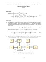
η

3
4

ξ

1

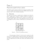
Figure 5.1.

2

Nodal strain gages for membrane.

Higher order strains.
The distribution of higher order strains is expressed in terms of natural strain
gage readings. The strain gage locations are placed at the 4 nodes (quadrilateral
corners). Readings along three directions are required. These directions are:
the ξ and η axis (quadrilateral medians) and the diagonal passing through the
neighboring nodes. See Figure 4.1.
The nodal natural strain readings are thus defined as








 ξ 
 ξ 

 ξ 
 ξ 
,
,
,
.
(5.2.27)
1 =
η
2 =
η
3 =
η
4 =
η








24

13

24

13

The next step is to connect these readings to the higher order degrees of freedom.
This can be done by defining a generic template
i

˜,
= Qi v

where Qi are 3 × 7 matrices. These templates are worked out below.

10

(5.2.28)


η
3

4

lη
lξ

ξ

d ξ|1
d η|1
1

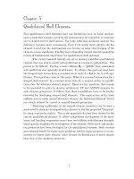
Figure 5.2.

2

Geometric dimensions for a quadrilateral element.

Higher order bending strain field.
The main displacement and strain mode that the field is trying to match is the
pure bending of the element along an arbitrary direction. The bending strain
field is associated with the higher order degrees of freedom θi , v˜ξ and v˜η . If one
considers pure bending of the element along the ξ direction, it seems intuitive
that the ξ strain should be proportional to the distance dξ from the ξ-axis. The ξ
strain should also be proportional to the curvature along the ξ-axis. In terms of
the rotational degrees of freedoms this curvature will have the form ∆θ/lξ where
lξ is the element length along the ξ-axis. The ξ strain thus gets coefficients of
the form dξ /lξ associated with the rotational degrees of freedom. Following a
similar reasoning for the η strains the strain distribution factors associated with
the ξ and η strains are established to be
χξ|i =

dξ|i
,
lξ

χη|i =

dη|i
,
lη

(5.2.29)

where
dξ|i =

(ri × sξ ) · (ri × sξ ) ,

lξ =

√

rξ · rξ ,

√

rξ =

1
(r2 + r3 − r1 − r4 ) ,
2

1
(r3 + r4 − r1 − r2 ) .
2
The quantities dξ|i , dη|i , lξ and lη are illustrated in Figure 4.2.
dη|i =

(ri × sη ) · (ri × sη ) ,

lη =

rη · rη ,

11

rη =


η
4

3

ξ

2

1

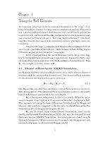
Figure 5.3.

Torsional mode for four node membrane element.

The strain distribution sensed by the diagonal strain gages are similarly
assumed to be proportional to the curvature along the diagonal, and proportional
to the distance from the diagonal as
χ24 =

d24
,
2l24

χ13 =

d13
,
2l13

(5.2.30)

where
d24 =

(r31 × e24 ) · (r13 × e24 ) ,

l24 =

d13 =

(r31 × e24 ) · (r13 × e24 ) ,

l13 =

√
√

r24 · r24 ,

r24 = (r2 − r4 ) ,

r13 · r13 ,

r13 = (r1 − r3 ) .

Torsional strain field.
The torsional strain field is associated to the θ¯ higher order degree of freedom.
As a guide for the construction of this strain field one can use the torsional
displacement mode illustrated in Figure 4.3. This figure indicates that this displacement mode should not induce shear strains, and that ξ should be positive
in 1st and 3rd quadrants and negative in 2nd and 4th. Similarly, η should be
positive in 2nd and 4th, and negative in 1st and 3rd quadrants. A simplified
strain distribution function for the strains ξ and η can thus be Nt = ξη.
With a unit rotation at all the nodes, the maximum displacement in the
ξ direction, uξ , will be proportional to the length lη . Since the strain ξ is the
gradient of the displacement uξ in the ξ direction this strain will be proportional
to 1/lξ . The torsional strain field is thus assumed to be
ξ

=α

lη
ξη = αχξt ξη,
lξ

η

= −α

12

lξ
ξη = −αχηt ξη.

lη

(5.2.31)


Generic nodal strain templates.
With the strain assumptions just described, the nodal strain gage readings can
be written down as
Q1 =

ρ1 χξ|1
 −ρ1 χη|1
ρ5 χ24
Q2 =

−ρ2 χξ|2
 ρ4 χη|2
ρ8 χ13
Q3 =

ρ3 χξ|3

 −ρ3 χη|3
ρ7 χ13
Q4 =

−ρ4 χξ|4
 ρ2 χη|4
ρ6 χ13

ρ2 χξ|1

ρ3 χξ|1

ρ4 χξ|1

αχξt

−ρ4 χη|1
ρ6 χ24

−ρ3 χη|1
ρ7 χ24

−ρ2 χη|1
ρ8 χ24

−αχηt
0

−ρ1 χξ|2

−ρ4 χξ|2

−ρ3 χξ|2

−αχξt

ρ1 χη|2
ρ5 χ13

ρ2 χη|2
ρ6 χ13

ρ3 χη|2
ρ7 χ13

αχηt
0

ρ4 χξ|3

ρ1 χξ|3

ρ2 χξ|3

αχξt

−ρ2 χη|3
ρ8 χ13

−ρ1 χη|3
ρ5 χ13

−ρ4 χη|3
ρ6 χ13

−αχηt
0

−ρ3 χξ|4

−ρ2 χξ|4

−ρ1 χξ|4

−αχξt

ρ3 χη|4
ρ7 χ13

ρ4 χη|4
ρ8 χ13

ρ1 χη|4
ρ5 χ13

αχηt
0

χ
−β1 χ¯ξξ|1
lξ

0
β2

c24ξ
l24

0

χ
,
−β1 χ¯ηη|1
lη
c
−β2 l24η
24

χ
−β1 χ¯ξξ|2
lξ

0

c13ξ
l13

χ
β1 χ¯ξξ|3
lξ

0

c13ξ
l13

χ
β1 χ¯ξξ|4

lξ

0
β2

c13ξ
l13

(5.2.34)


β1 χη|3
χ
¯ η lη
c
β2 l13η
13

0
−β2

(5.2.33)


χ
,
β1 χ¯ηη|2
lη
c13η
β2 l13

0
−β2

(5.2.32)


0


,

(5.2.35)


χ
,
−β1 χ¯ηη|4
lη
c
−β2 l13η
13

where c13ξ = sT13 sξ , c13η = sT13 sη , c24ξ = sT24 sξ and c24η = sT24 sη .
The cartesian strain displacement matrices at the nodes are obtained by
the transformations
 2

sξ x sξ y
sξ x sξ 2y

Bh1 = T13 Q1 ,
 sη 2 sη 2
where T−1
sη x sη y  ,
(5.2.36)
13 =
x
y
Bh3 = T13 Q3 ,
2
2
s24 x s24 y s24 x s24 y


Bh2 = T24 Q2 ,
Bh4 = T24 Q4 ,

where

T−1
24

sξ 2x
=  sη 2x
s13 2x

13

sξ 2y
sη 2y

s13 2y


sξ x sξ y
sη x sη y  .
s13 x s13 y

(5.2.37)


A higher order strain field over the element can now be obtained by interpolating
the nodal Cartesian strains by use of the bi-linear shape functions defined in
(5.1.3).
Bh (ξ, η) =

(1 − ξ)(1 − η)Bh1 + (1 + ξ)(1 − η)Bh2
+(1 + ξ)(1 + η)Bh3 + (1 − ξ)(1 + η)Bh4 .

(5.2.38)

Interpolation of these nodal strains does not automatically give a deviatoric
higher order strain field. Such a condition can be achieved by subtracting the
mean strain values:
¯h
Bd (ξ, η) = Bh (ξ, η) − B

where

¯h =
B

B(ξ, η) dA .

(5.2.39)

A

Optimal coefficients for the strain computation.
When computing the strain displacement expressions symbolically using Mathematica, the contributions of the different coefficients ρi and βi were evaluated
with respect to certain higher order strain modes. Based on pure bending of
rectangular element shapes the following dependencies between the coefficients
were obtained:
ρ2 = −ρ1 ,
ρ3 = ρ2 ,
ρ4 = ρ1 ,
1
(5.2.40)
ρ6 = β1 − ρ1 ,
β1 = + ρ1 ,
2
ρ8 = −ρ6 ,
ρ5 = ρ7 = β2 = 0 .
As seen this makes all the coefficients a function of ρ1 . Optimizing ρ1 with
respect to irregular meshes for the cantilever described in the numerical section
suggests ρ1 = 0.1 , and the following set of optimal coefficients:
ρ1 = 0.1
ρ5 = 0.0

ρ2 = −0.1
ρ6 = 0.5

β1 = 0.6

ρ3 = −0.1 ρ4 = 0.1
ρ7 = 0.0 ρ8 = −0.5
β2 = 0.0

14

(5.2.41)


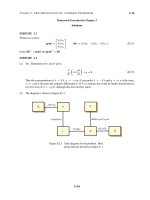
Figure 5.4.

4

3

1

2

Spurious membrane mode for the four node
ANDES element.

Stiffness computation for the membrane element.
According to the ANDES formulation the element stiffness is computed as
K=

1
˜ dH

LCLT + HT K
A

where

˜d =
K

BTd CBd dA .

(5.2.42)

A

Numerical experiments, however, indicate that the element performs better when
the element stiffness is computed as
K=

1
˜ hH
LCLT + HT K
A

where

˜h =
K

BTh CBh dA ,

(5.2.43)

A

that is when the non-deviatoric higher order strains are used. This is not strictly
justified according to the standard ANDES formulation since the higher order
strains displacement matrix Bh is not energy orthogonal with respect to the
constant strain modes for arbitrary element geometries. However, both of the
above element stiffness matrices satisfy the Individual Element Test and thus
also the conventional Patch Test.
Rank of the stiffness matrix.
Performing an eigenvalue analysis of the element stiffness matrices given in equations (5.2.42) and (5.2.43) it was found that the element has one spurious zero
energy mode in addition to the correct three rigid body modes. This spurious
mode occurred using a 2×2 Gauss integration rule. It is expected that this spurious mode would disappear with a 3×3 integration rule. For a square element

15


as shown in Figure 5.4 this spurious mode is defined by the nodal displacement
pattern
vT = [ vx1

vx2

vx3

vx4

= [ 1 −1

−1

1

vy1

vy2

vy4

θz1

θz2

1

1

4 −4

θz3

θz4 ]

−4 ] .
(5.2.44)
Analysis of a mesh of two elements shows that this the pattern (5.2.44) can
not occur in a mesh of more than one element. The spurious mode is then not
practically significant for the performance of the element.

5.3

−1 −1

vy3

4

The quadrilateral bending element.

The current approach to deriving the quadrilateral plate bending element utilizes
reference lines. Hrennikoff [00] first used this concept for plate modeling where
the goal was to come up with a beam framework useful as a model for bending
of flat plates.
Park and Stanley [ 00, 00] used the reference line concept in their development of several plate and shell elements based on the ANS formulation. The
reference lines were used to find beam-like curvatures; these curvatures were
then used to find the plate curvatures through various Assumed Natural Strain
distributions. These plate and shell elements were of Mindlin-Reissner type, and
the reference lines were treated as Timoshenko beams.
The present element is a Kirchhoff type plate and the reference lines are
thus treated like Euler-Bernoulli (or Hermitian) beams.
5.3.1 Basic stiffness.
The basic stiffness for a flat quadrilateral bending element has been developed
by extending the triangle element lumping matrices Ll and Lq of Militello to
four node elements. Ll and Lq denotes lumping with respect to a linear and
quadratic variation in the normal side rotation respectively.
By ordering the element degrees of freedom as rotation about x and y
axis and translation in z direction for each node one obtains the lumped forces
from bending as



 mxx 
f = Ll σ or f = Lq σ where σ = myy ,
(5.3.1)


mxy





Ll 1
L 
Ll =  l 2  ,
Ll 3
Ll 4


Lq 1
L 
Lq =  q 2 
Lq 3
Lq 4
16

(5.3.2)


and

 
f1


 
f1
f=


 f1 
f1

where



 mx 
f i = my .


fz

(5.3.3)

The lumped node forces at a node j given by lumping matrix Lj , receive contributions from the moments from adjoining sides ij and jk. The lumped force
vector at a node j is thus a function of the coordinates of the sides ij and jk
only. With linear interpolation of the normal and tangential rotations along a
side the lumping matrix becomes


Ll j

0
1
=
0
2
−yki

0
−xki
0


0
yki  ,
−xki

(5.3.4)

where superscript l denotes linear variation of normal rotation. If the normal
rotation is assumed to vary quadratically in accordance to Hermitian interpolation whereas and the tangential rotation still varies linearly the lumping matrix
becomes


−cjk sjk + cij sij
cjk sjk − cij sij
−(s2jk − c2jk ) + (s2ij + s2ij )


Lq =  1 (s2jk xjk + s2ij xij ) 1 (c2jk xjk + c2ij xij )
−c2jk yjk − c2ij yij
j

2
1 2
2 (sjk yjk

+ s2ij yij )

2
1 2
2 (cjk yjk

+ c2ij yij )

−s2jk xjk − s2ij xij

(5.3.5)
where superscript q is used to denote quadratic variation of normal rotations.
The nodal indices (i, j, k, l) in the equations above undergo cyclic permutations
of (1, 2, 3, 4) as for the membrane lumping.
5.3.2 Higher order stiffness
The higher order stiffness is computed as the deviatoric part of an ANS type
element using the Euler-Bernoulli beam as a reference line strain guide.

17


Nodal curvatures of a Euler-Bernoulli beam.

The transverse displacement of a Euler-Bernoulli beam, written as a function of
the nodal displacements and rotations is
w = Nw vbij ,
where



2 ( 2 + ξ)(−1 + ξ)2 

1  l ( 1 + ξ)(−1 + ξ)2 
T
N =
2
8

 2 ( 2 − ξ)( 1 + ξ)2 
l (−1 + ξ)( 1 + ξ)

(5.3.6)

and vb ij



wi 



θni
=

.

 wj 

θnj

The beam curvatures are


6ξ



1 l (−1 + 3ξ) 
∂2w
= 2
vb ij ,
κ=
−6ξ


∂x2
l 

l (−1 + 3ξ)

(5.3.7)

The nodal curvatures are then
κij|i

κij|j

=

−6
6

1
l2

−4l
2l

6
−6

−2l
v
4l bij

(5.3.8)

The nodal displacements of a reference-line from node i to j can be expressed
in terms of the visible degrees of freedom at those nodes as
vb ij = Tvij vij
 1

wi 

 0


θn i
=
0
w


j


0
θn j

0

0

nij x
0
0

nij y
0
0

0
0
0
0
1

0
0 nij x

(5.3.9)


w


i





0
θ


xi 




0  θy i 
.
wj 
0 





nij y 
θy 



θ j 


(5.3.10)

yj

The nodal curvatures expressed in terms of the visible dofs at node i and j then
become
κij|i
κij|j

=

1
l2

−6
6

−4l nij x
2l nij x

−4l nij y
2l nij y

18

6
−6

−2l nij x
4l nij x

−2l nij y
v.
4l nij y
(5.3.11)


η
3
4

ξ

1

Figure 5.5.

2

Nodal curvature gages for bending.

Nodal natural coordinate curvatures for a quadrilateral.
When one collects all the nodal straingages in a vector g, the strain-gage displacement relationship becomes
g = Qv = QF ∗Fv ,

(5.3.12)

where ∗ denotes entry by entry matrix multiplication, and
gT = [ κ41|1

κ12|1

κ13|1

κ12|2

κ23|2

κ24|2

κ23|3

κ34|3

κ13|3

κ34|4

κ41|4

κ24|4 ] ,

(5.3.13)


−6
4
4
0
0
0
0
0
0
6
2
2
6 −2 −2
0
0
0
0
0
0 
 −6 −4 −4


0
0
0

6 −2 −2
0
0
0 
 −6 −4 −4






2
2 −6
4
4
0
0
0
0
0
0 
 6


0
0 −6 −4 −4
6 −2 −2
0
0
0 

 0


0
0 −6 −4 −4
0
0
0
6 −2 −2 
 0


QF = 
,


0
0
6
2
2 −6
4
4
0
0
0 
 0


0

0
0
0
0 −6 −4 −4
6 −2 −2 
 0


2
2
0
0
0 −6
4
4
0
0
0 
 6






0
0
0
0
0

0
6
2
2
−6
4
4




6 −2 −2
0
0
0
0
0
0 −6 −4 −4
0
0
0
6
2
2
0
0
0 −6
4
4
(5.3.14)



19




F41
 F12

 F13



 F12

 F23

 F24

F=

 F23

 F34

 F13




 F34

F41
F24

F41
F12
F13

F41
F12
F13

F12
F23
F24

F12
F23
F24

F23
F34
F13

F23
F34
F13

F34

F41
F24

F34
F41
F24


F41
F12 

F13 



F12 

F23 

F24 



F23 

F34 

F13 




F34 

F41
F24

F12 =
F23 =
where

F34 =
F41 =
F13 =
F24 =

1
2
l12
1
2
l23
1
2
l34
1
2
l41
1
2
l13

1
2
l24

n12 x
l12
n23 x
l23
n34 x
l34
n41 x
l41
n13 x
l13
n24 x
l24

n12 y
l12
n23 y
l23
n34 y
l34
n41 y
l41
n13 y
l13
n24 y
l24

. (5.3.15)

Cartesian curvatures for a quadrilateral.
The cartesian curvatures κT = [ κxx κyy κxy ] at the nodes can now be obtained as
gC = QC v
(5.3.16)
or


 



κ
B1
Tκ 1 Q1

 |1 

κ|2
B 
T Q 
=  2  v =  κ2 2  v ,
B3
Tκ 3 Q3

 κ|3 

κ|4
B4

Tκ 4 Q4


where
Tκ −1
1
Tκ −1
2
Tκ −1
3
Tκ −1
4

s41 2x
=  s12 2x
s13 2x
 2
s12 x

= s23 2x
s24 2x
 2
s23 x

= s34 2x
s13 2x
 2
s34 x

= s41 2x

s24 2x

s41 2y
s12 2y
s13 2y
s12 2y
s23 2y
s24 2y
s23 2y
s34 2y
s13 2y
s34 2y
s41 2y
s24 2y


s41 x s41 y
s12 x s12 y  ,
s13 x s13 y

s12 x s12 y
s23 x s23 y  ,
s24 x s24 y

s23 x s23 y
s34 x s34 y  ,
s13 x s13 y

s34 x s34 y
s41 x s41 y  .

s24 x s24 y

The Cartesian curvatures over the element can then be obtained by interpolation
of the nodal values as
κ = B(ξ, η)v ,
(5.3.17)
20


where
B(ξ, η) =

(1 − ξ)(1 − η)B1 + (1 + ξ)(1 − η)B2
+(1 + ξ)(1 + η)B3 + (1 − ξ)(1 + η)B4

.

(5.3.18)

Higher order stiffness for the element.
The ANDES higher order stiffness is computed as
BTd CBd dA

Kd =

where

Bd = B −

A

1
A

B dA .

(5.3.19)

A

5.3.3 The ANS quadrilateral plate bending element.
Clearly one can form an ANS type element by
BT CB dA

K=

(5.3.20)

A

i.e. without extracting the mean part of the strain displacement matrix and not
including the basic stiffness described in Section 5.3.1.

5.4

The linear non-flat quadrilateral shell element.

The objective of this section is to develop a technique that allows the use of
the flat quadrilateral membrane and bending element as parts of a non-flat shell
element for linear problems. This is obtained by formulating a linear projector matrix, which for the linear case restores equilibrium at the undeformed

element geometry. This can also be obtained by using the nonlinear projector
with respect to the initial geometry. In fact the linear and nonlinear projector gives identical results for linear problems. However the linear projector is
recommended for linear finite element codes due to its greater simplicity.
The four node shell element is obtained by assembling the membrane
element and bending element to the appropriate degrees of freedom. This is
sufficient as long as the shell element is strictly flat since both the membrane
and bending elements are developed as flat elements. Unfortunately, four node
shell elements on a “real” structure quite often end up being warped. To restore
or improve the behavior of the warped element one can use a projection technique
similar to that developed by Rankin and coworkers [ 00, 00].
The element stiffness matrix does not have the correct rigid body modes
if the element geometry is warped since the element stiffness has been developed
using the projected flat positions of the element nodes. This causes two deficiencies of the element stiffness:
1. The element picks up strains and thus forces from a rigid body displacement vector i.e. f r = Kvr = 0.
21


2. The element forces are not in self equilibrium and the force vector will
thus pick up energy for a rigid body motion. vTr f = vTr Kv = 0.
These two statements are equivalent for a symmetric element stiffness matrix.
If an element stiffness has columns that are in self equilibrium the element has
the correct rigid body modes and vice versa.
The foregoing deficiencies lead to the investigation of the element internal energy
1
1
Φ = vT Kv = (vTr + vTd )K(vr + vd )
2
2
(5.4.1)
1 T

= (vd Kvd + vTd Kvr + vTr Kvd + vTr Kvr ).
2
If the element fails the equilibrium and rigid-body conditions;
vTr Kvr = 0 ,

vTr Kvd = 0

and vTd Kvr = 0 .

(5.4.2)

To extract the deformational energy, the total displacements are split into deformational and rigid body motions, the latter being spanned by the matrix
R:
v = vd + vr = vd + Ra.
(5.4.3)
By requiring that the deformational displacement vector be orthogonal to the
rigid body modes one must have RT vd = 0. On pre-multiplying the equation
above with RT the rigid body amplitudes can be solved for:
RT v = RT Ra

a = ( RT R )−1 Rv ,

⇒

(5.4.4)

from which the deformational displacement vector can be extracted as
vd = v − vr = ( I − R ( RT R )−1 R ) v = Pd v.

(5.4.5)

If R is orthonormal the foregoing expression simplifies to
Pd = I − RRT .

(5.4.6)

Applying this projection to gain invariance of the internal energy with
respect to rigid body motion Φ(v) = Φ(vd ) yields
Φ(vd ) =

1 T
1
1
vd Kvd = vT PTd KPd v = vT Kd v .
2
2
2

22

(5.4.7)


5.4.1 Linear projector matrix for a general quad.
In order to express the rigid body modes one defines the vector ri from the
element centroid to node i as
 
4
 xi 
1

˜ri = ri − ¯r , where ri = yi
ri .
(5.4.8)
and ¯r =
 
4 i=1
zi
By ordering the element degrees of freedom as
 
v

 1

v2
v=

 v3 

v4

where



vxi 




v 




 yi 

vzi
vi =

 θxi 






 θyi 

θzi

(5.4.9)

the rigid body modes can be expressed as






R1
 R2 

R=
,
R3
R4

I
0

Ri =

1
0

−Spin(˜ri )
0
=
I
0

0
0

0
1
0
0
0
0

0

0
1
0
0
0

0
−˜
zi
y˜i
1
0
0

z˜i
0
−˜
xi
0
1
0


−˜
yi
x
˜i 

0 
.

0 

0
1
(5.4.10)

The projector matrix becomes
Pd = I − R(RT R)−1 RT ,
where
4I
R R=
0
T

0
S

(5.4.11)

4

with S = 4I −

Spin(˜ri )Spin(˜ri ) .
i=1

This simplifies the computation of the projector matrix because only the lowest
3×3 submatrix of RT R is non-diagonal, and (RT R)−1 can be efficiently formed.

23

5.5

Nonlinear extensions for quadrilateral shell element.

The nonlinear extensions for an element consists of defining a procedure that
aligns the shadow element C0n as close as possible to the deformed element Cn .
This defines the element deformational displacement vector vd .
One also needs to form the rotational gradient of the shadow element
with respect to the visible degrees of freedom of the deformed element, as stated
in equation (0.0.0). In the local coordinate system this relation is
˜r =
δω

˜r
∂ω
˜ δ˜
δvi = G
v.
∂˜
vi

(5.5.1)

The local coordinate relationship is sought since this is is needed in forming the
geometric stiffness of the element as expressed in equation (0.0.0) .
The rotation of the shadow element is most easily obtained from the
rotation of the shared or common local frame for the C0n and Cn configurations.
This orthogonal element coordinate frame with unit axis vectors e1 , e2 and e3

is rigidly attached to the shadow element C0n , since this element only moves
as a rigid body, and elastically attached to the deformed and elastic element
Cn . This local coordinate system for a quadrilateral element can be defined in
various ways. Most researchers select the element z-axis unit vector as the cross
product of the diagonals vectors d13 and d24
e3 =

d13 × d24
Ap

where

(d13 × d24 )T (d13 × d24 )

Ap =

(5.5.2)

This defines Ap as the area of the element projection on the local x − y plane.
The positioning of the x and y axis unit vectors e1 and e2 differs among
researchers. Rankin and Brogan [00] chooses e2 to coincide with the projection
of the side edge 24 on the plane normal to e3 . This effectively lets only one of the
side edges determine the rigid rotation of the element about the local z axis. The
origin of the element coordinate system is chosen to coincide with node 1. When
this procedure is performed for both the C0 and Cn element configurations the
net result is that the shadow element C0n will be positioned relative to Cn so that
nodes 1 coincide and the projections of side edge 24 on the (x, y) plane coincide.
A consequence of this choice is that the element deformational displacement
vector vd , which is the difference between the coordinate between the Cn and
C0n coordinates, is not invariant with respect to the element node numbering.

Bergan and Nyg˚
ard [00] choose vector e1 and e2 to coincide with the
directions of side edge 12 and 14 for a rectangle that is positioned relative to
the quadrilateral element so that the sum of the angles between the side edges
of the quadrilateral and rectangle is zero. The origin of the coordinate system
24


is chosen at node 1. By applying this to both the C0 and Cn configurations the
shadow element C0n is positioned relative to the deformed element Cn so that
the element centroids coincide and so that the sum of the square of the angles
between the side edges of C0n and Cn is minimized. This represents a least
square fit with respect to the side edge angular errors. This procedure gives a
element deformational displacement vector vd which produces an internal force
vector f e = Ke vd that is invariant with respect to the node numbering of the
element, provided that the element stiffness matrix Ke satisfies the correct rigid
body translations.
5.5.1 Aligning side 12 of C0n and Cn .
The element frame is positioned at the element centroid. This change from
Rankin’s positioning at node 1 has been done in order to satisfy the orthogonality
condition for PT PR = 0 as expressed in equation (0.0.0) . Rankin’s formulation
did not contain PT so this requirement was ignored.
By expressing the nodal coordinates of the element in the local coordinate system equation (5.5.2) gives




y˜31 z˜42 − y˜42 z˜31 
 e˜3x 


1
˜3 = e˜3y =
e
−˜
x31 z˜42 + x
˜42 z˜31 ,

 Ap 

e˜3z
x
˜31 y˜42 − x
˜42 y˜31

(5.5.3)

where
(˜
y31 z˜42 − y˜42 z˜31 )2 + (−˜
x31 z˜42 + x
˜42 z˜31 )2 + (˜
x31 y˜42 − x
˜42 y˜31 )2 .
(5.5.4)
These expressions simplify, but the full expressions has to be kept in order to
obtain the correct variation with respect to the nodal coordinates. The ω
˜ x and
ω
˜ y variation can now be obtained from the variation of e3y and e3x respectively
Ap =

∂˜
e3y
δx
˜i +
∂x
˜i
∂˜
e3x
(
δx
˜i +
∂x
˜i

δω
˜ x = −(
δω
˜y =

∂˜
e3y
∂˜
e3y
δ y˜i +
δ˜
zi ) ,
∂ y˜i
∂ z˜i
∂˜

e3x
∂˜
e3x
δ y˜i +
δ˜
zi ) .
∂ y˜i
∂ z˜i

(5.5.5)

The variation of ω
˜ x and ω
˜ y with respect to the in-plane coordinate components
of the nodes x
˜i and y˜i is zero since
∂˜
e3x
∂˜
e3x
∂˜
e3y
∂˜
e3y
=
=
=
=0.
∂x
˜i

∂ y˜i
∂x
˜i
∂ y˜i

25

(5.5.6)