The proper generalized decomposition for advanced numerical simulations ch16

16

.

The Ten Node
Tetrahedron

16–1


16–2

Chapter 16: THE TEN NODE TETRAHEDRON

TABLE OF CONTENTS
Page

§16.1. INTRODUCTION

16–3

§16.2. THE QUADRATIC TETRAHEDRON
§16.3. PARTIAL DERIVATIVE CALCULATIONS
§16.3.1. Implementation Considerations
. . . . . . . . . . .
§16.4. GAUSS RULES OVER TETRAHEDRA

16–3
16–4
16–6
16–8

§16.5. THE ELEMENT STIFFNESS MATRIX

16–8

§16.6. THE CONSISTENT NODE FORCE VECTOR

16–9

EXERCISES

. . . . . . . . . . . . . . . . . . . . . .

16–2

16–10


16–3

§16.2

THE QUADRATIC TETRAHEDRON

§16.1. INTRODUCTION
The technique used in Chapter 15 for the derivation of the linear triangle is now extended to the
10-node tetrahedron, also called the quadratic tetrahedron. This element can have curved faces and
edges. The extension is based on the isoparametric technique and the partial-derivative construction
procedure followed the IFEM course for the 6-node triangle.
§16.2. THE QUADRATIC TETRAHEDRON

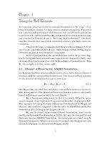
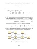
The ten node tetrahedron shown in Figure 16.1 is the next complete-polynomial member of the
isoparametric tetrahedron family.
The element has four corners with local numbers 1 through 4, which must be traversed following the
same convention as the four node tetrahedron. It has six side nodes, with local numbers 5 through
10; nodes 5,6,7 are located on sides 1-2, 2-3 and 3-1, whereas nodes 8,9,10 are located on sides 1-4,
2-4, and 3-4. The side nodes may be located arbitrarily subjected to positive-Jacobian-determinant
constraints. Each element face is defined by six nodes, which are not necessarily on a plane.
The isoparametric element definition is


1
1
 x1

 x   y1
  
 y  =  z1
  
ux
 u x1

uy
u y1
u z1




1
x2

y2
z2
u x2
u y2
u z2

1
x3
y3
z3
u x3
u y3
u z3

1
x4
y4
z4
u x4
u y4
u z4

  (e) 
...
1
N1
. . . x10   N2(e) 


. . . y10   N (e) 

 3 
. . . z 10   N (e)  .


. . . u x10   .4 
  .. 
. . . u y10
(e)
N10
. . . u z10

(16.1)

The conventional (non-hierarchical) shape functions are
N1(e) = ζ1 (2ζ1 − 1),

N2(e) = ζ2 (2ζ2 − 1)

N3(e) = ζ3 (2ζ3 − 1),

N4(e) = ζ4 (2ζ4 − 1)

N5(e) = 4ζ1 ζ2 ,

N6(e) = 4ζ2 ζ3

N7(e) = 4ζ3 ζ1 ,

N8(e) = 4ζ1 ζ4

N9(e) = 4ζ2 ζ4 ,

(e)
N10
= 4ζ3 ζ4

.

(16.2)

These shape functions are similar in form to those of the six node quadratic triangle discussed in
IFEM. If the element is curved (that is, the six nodes that define each face are not on a plane), the
tetrahedron coordinates no longer fall on planes, but form a curvilinear system.

16–3


16–4

Chapter 16: THE TEN NODE TETRAHEDRON

4
8
z

10
7

1

3

9
6

5
x

2

y

Figure 16.1. The ten-node (quadratic) tetrahedron

§16.3. PARTIAL DERIVATIVE CALCULATIONS
The main task involved in writing the shape function subroutine for the 10-node tetrahedron is the
computation of the partial derivatives of the functions in (16.1) with respect to x, y and z at any
point in the element. For this purpose consider a generic scalar function, w(ζ1 , ζ2 , ζ3 , ζ4 ), that is
quadratically interpolated over the ten-node tetrahedron with the shape functions (16.2):


w = [ w1

w2

w3

w4

w5

w6

...


ζ1 (2ζ1 − 1)
 ζ2 (2ζ2 − 1) 


 ζ3 (2ζ3 − 1) 


 ζ4 (2ζ4 − 1) 

w10 ]  4ζ1 ζ2 
.


 4ζ2 ζ3 


..


.

(16.3)

4ζ3 ζ4

Symbol w may represent x, y, z, u x , u y or u z in the isoparametric representation (7.1), or other
element-varying quantities such as body forces or temperatures.
Taking partials with respect to x, y and z, and applying the chain rule twice we get
∂w
=
∂x
∂w
=
∂y
∂w
=
∂z

∂ Ni
=
∂x
∂ Ni
wi
=
∂y
∂ Ni
wi
=
∂z
wi

wi
wi
wi

∂ Ni
∂ζ1
∂ Ni
∂ζ1
∂ Ni
∂ζ1

∂ζ1
∂ Ni ∂ζ2
∂ Ni ∂ζ3
∂ Ni
+
+
+
∂x
∂ζ2 ∂ x
∂ζ3 ∂ x
∂ζ4
∂ζ1
∂ Ni ∂ζ2
∂ Ni ∂ζ3
∂ Ni
+
+
+
∂y
∂ζ2 ∂ y
∂ζ3 ∂ y
∂ζ4

∂ζ1
∂ Ni ∂ζ2
∂ Ni ∂ζ3
∂ Ni
+
+
+
∂z
∂ζ2 ∂z
∂ζ3 ∂z
∂ζ4
16–4

∂ζ4
∂x
∂ζ4
∂x
∂ζ4
∂x

,
,
,

(16.4)


16–5

§16.3

PARTIAL DERIVATIVE CALCULATIONS

where all sums are understood to run from i = 1 through 10, and element superscripts on the shape
functions have been suppressed for clarity. In matrix form:
 ∂w
∂x
 ∂w

 ∂y
∂w
∂z

  ∂ζ1
∂x
 

 =  ∂ζ1
  ∂y
∂ζ1
∂z

∂ζ2
∂x
∂ζ2
∂y
∂ζ2
∂z

∂ζ3

∂x
∂ζ3
∂y
∂ζ3
∂z



∂ζ4 
∂x  

∂ζ4  

∂y  


∂ζ4 
∂z

wi ∂∂ζNi
1

wi ∂∂ζNi
2
∂
N
wi ∂ζ i
3
wi ∂∂ζNi
4











(16.5)

Transposing both sides of (16.5) while switching the left and right hand sides, yields a form exploited
below:
 ∂ζ1 ∂ζ1 ∂ζ1 
∂x
∂y
∂z


 ∂ζ2 ∂ζ2 ∂ζ2 

∂y
∂z 

∂ Ni  ∂ x
∂w ∂w .
wi ∂∂ζNi
wi ∂∂ζNi

wi ∂∂ζNi
= ∂w

∂x
∂y
∂z
∂ζ4  ∂ζ3 ∂ζ3 ∂ζ3 
1
2
3


 ∂x
∂y
∂z 

∂ζ4 ∂ζ4 ∂ζ4
∂x
∂y
∂z
(16.6)
Now make w ≡ x, y, z and stack the results row-wise:






xi ∂∂ζNi
1

yi ∂∂ζNi
1

z i ∂∂ζNi
1

xi ∂∂ζNi
2

yi ∂∂ζNi
2

z i ∂∂ζNi
2

xi ∂∂ζNi
3

yi ∂∂ζNi
3

z i ∂∂ζNi
3

 ∂ζ1
∂x

xi ∂∂ζNi 
 2

4
  ∂ζ

 ∂x
∂
N
yi ∂ζ i  
4   ∂ζ3
 ∂x
∂
N
z i ∂ζ i 
4
∂ζ4
∂x

∂ζ1
∂y
∂ζ2
∂y
∂ζ3
∂y
∂ζ4
∂y

∂ζ1
∂z
∂ζ2
∂z
∂ζ3

∂z
∂ζ4
∂z




 ∂ζ1
1
∂x

∂
N
i


xi ∂ζ   ∂ζ2
4
  ∂x

∂
N
i
yi ∂ζ   ∂ζ3
4 
 ∂x
z i ∂∂ζNi
∂ζ4
4
∂x

∂ζ1
∂y
∂ζ2
∂y
∂ζ3
∂y
∂ζ4
∂y

∂ζ1
∂z
∂ζ2
∂z
∂ζ3
∂z
∂ζ4
∂z



  ∂x

  ∂x
  ∂y
 =  ∂x


∂z


∂x

∂x
∂y
∂y
∂y
∂z
∂y

∂x
∂z
∂y
∂z
∂z
∂z



.


(16.7)
This is a linear system with the required unknowns in the second matrix, but its coefficient matrix
is not square. To achieve that, differentiate both sides of the identity ζ1 + ζ2 + ζ3 + ζ4 = 1 with
respect to x, y and z, and insert as first row:
 ∂1
∂x

  ∂x
 

  ∂x
 =  ∂y
 
  ∂x

∂z
∂x

∂1 
∂z

∂
x


1
2
3
∂z 

.

∂N
∂y 
yi ∂∂ζNi
yi ∂∂ζNi

 yi ∂ζ i
1
2

3

∂z 
∂
N
∂
N
∂
N
∂z
i
i
i
z i ∂ζ
z i ∂ζ
z i ∂ζ
∂z
1
2
3
(16.8)
But ∂ x/∂ x = ∂ y/∂ y = ∂z/∂z = 1 and ∂1/∂ x = ∂1/∂ y = ∂1∂z = ∂ x/∂ y = ∂ x/∂z = ∂ y/∂ x =
∂ y/∂z = ∂z/∂ x = ∂z/∂ y = 0 because x, y and z are independent coordinates. Consequently we


1
xi ∂∂ζNi

1
xi ∂∂ζNi

1
xi ∂∂ζNi

16–5

∂1
∂y
∂x
∂y
∂y
∂y
∂z
∂y


16–6

Chapter 16: THE TEN NODE TETRAHEDRON

arrive at a system of linear equations of order 4 with three right-hand sides.
convention to get rid of sum symbols the system is
 ∂ζ1 ∂ζ1 ∂ζ1 
 1
1
1
1  ∂x
∂y
∂z
 


∂
N
∂
N
∂
N
∂
N
i
i
i
i
0
  ∂ζ2 ∂ζ2 ∂ζ2 
 xi
x
x
x
i
i
i
 ∂ζ1
∂ζ2
∂ζ3
∂ζ4   ∂ x
∂y
∂z 
 1



=

 ∂ Ni
0
yi ∂∂ζNi yi ∂∂ζNi yi ∂∂ζNi   ∂ζ3 ∂ζ3 ∂ζ3 
 yi ∂ζ

1
2
3
4 

∂
x
∂
y
∂z
0


∂
N
∂
N
∂
N
∂
N
i

i
i
i
z i ∂ζ
z i ∂ζ
z i ∂ζ
z i ∂ζ
∂ζ4 ∂ζ4 ∂ζ4
1
2
3
4
∂x
∂y
∂z

Using the summation

0
0
1
0


0
0
.
0
1

(16.9)

In compact matrix notation
JP = Iaug .
where

(16.10)



1
1
1
1 
1
1
1
1
 x i ∂ Ni x i ∂ Ni x i ∂ Ni x i ∂ Ni 
∂ζ1
∂ζ2
∂ζ3
∂ζ4 
Jx2 Jx3 Jx4  
J
J =  x1
(16.11)
=
∂
N

∂
N
∂
N
∂
Ni 
i
i
i

.
Jy1 Jy2 Jy3 Jy4
 yi ∂ζ1 yi ∂ζ2 yi ∂ζ3 yi ∂ζ4 
Jz1 Jz2 Jz3 Jz4
z i ∂∂ζNi z i ∂∂ζNi z i ∂∂ζNi z i ∂∂ζNi
1
2
3
4
and Iaug is the 3 × 3 identity matrix augmented with a zero first row. Taking the partials of the shape
functions (16.2) with respect to the tetrahedron coordinates and substituting into the above yields




Jx1 = x1 (4ζ1 − 1) + 4x5 ζ2 + 4x7 ζ3 + 4x8 ζ4 ,
Jx2 = x2 (4ζ2 − 1) + 4x6 ζ3 + 4x5 ζ1 + 4x9 ζ4 ,
Jx3 = x3 (4ζ3 − 1) + 4x7 ζ1 + 4x6 ζ2 + 4x10 ζ4 ,
Jx4 = x4 (4ζ4 − 1) + 4x8 ζ1 + 4x9 ζ2 + 4x10 ζ3 .

(16.12)

For Jyi and Jzi replace xi by yi and z i , respectively, into the above formulas.
Summarizing, to compute the x-y-z partials for a function w interpolated as per (16.3) the recipe
is: form the linear system (16.10) from the geometric data, solve for the 12 tetrahedron coordinates
partials, and substitute these into (16.5).
REMARK 16.1

By analogy with the isoparametric brick elements, matrix J of (16.10) may be called a Jacobian matrix.
However, the factor J that appears in the element-of-volume transformation
d V (e) = J dζ1 dζ2 dζ3 ζ4 ,

(16.13)

is not det J = |J|, but J = 16 |J. If the element has straight sides with side nodes at the midpoints, J is constant
and equal to the volume V of the tetrahedron, which is given by the usual formula
J =V=

1
6

1
x1
y1
z1

1
x2
y2
z2

as in Chapter 6. In this case J is constant over the element.

16–6

1
x3
y3
z3

1
x4
,
y4
z4

(16.14)


16–7

§16.3

PARTIAL DERIVATIVE CALCULATIONS

§16.3.1. Implementation Considerations
To speed up computations in the shape function subroutine it is important to observe that the
Jacobian matrix has the special structure (16.11). We can take advantage of this by subtracting the
first column of J from the last three columns. This manipulation reduces (16.10) to the solution of
a 3 × 3 linear system:

Jx2 − Jx1
Jy2 − Jy1
Jz2 − Jz1

Jx3 − Jx1
Jy3 − Jy1
Jz3 − Jz1

Jx4 − Jx1
Jy4 − Jy1
Jz4 − Jz1

 ∂(ζ − ζ )
2
1
∂
x

 ∂(ζ3 − ζ1 )

∂x

∂(ζ4 − ζ1 )
∂x

or

∂(ζ2 − ζ1 )
∂y
∂(ζ3 − ζ1 )

∂y
∂(ζ4 − ζ1 )
∂y

∂(ζ2 − ζ1 ) 
∂z

∂(ζ3 − ζ1 ) 
=
∂z

∂(ζ4 − ζ1 )
∂z

J¯ P¯ = I

1
0
0

0
1
0

0
0
1

(16.15)
(16.16)

where I is the 3 × 3 identity matrix, and the modified Jacobian matrix is shown on the left hand
¯ which can be readily calculated by Cramer’s rule. Finally,
side. Therefore P¯ is just the inverse of J,
the first row of P is recovered from the constraints
∂ζ2
∂ζ3
∂ζ4
∂ζ1
+
+
+
= 0,
∂x
∂x
∂x
∂x

(16.17)

and similarly for the y and z partials. This is done as follows: take the column sum sx of the
¯ then
computed first column of P;
∂ζ1
= − 14 sx ,
(16.18)
∂x
from which the other x can be recovered. This operation is repeated over the other columns.
To tie up with the notation used in Chapter 6 for the four-node tetrahedron, we may denote the
partials as

 ∂ζ1
∂x

 ∂ζ2
 ∂x


 ∂ζ3
 ∂x

∂ζ4
∂x

∂ζ1
∂y
∂ζ2
∂y
∂ζ3
∂y
∂ζ4
∂y

∂ζ1
∂z
∂ζ2
∂z
∂ζ3
∂z
∂ζ4
∂z




a1


1 a

=  2

J a3

a4


b1
b2
b3
b4


c1
c2 

c3
c4

(16.19)

For the 4-node tetrahedron, J = 16 V was constant over the element, but now it generally will vary
with position unless the tetrahedron has planar faces.

16–7


16–8

Chapter 16: THE TEN NODE TETRAHEDRON

§16.4. GAUSS RULES OVER TETRAHEDRA
We mention the first two numerical integration rules, which find applications in the evaluation of
element stiffness matrix and consistent force vector.
One point rule (exact for constant and linear polynomials over plane-face tetrahedra):
1
V

V (e)

F(ζ1 , ζ2 , ζ3 , ζ4 ) d V (e) ≈ F( 14 , 14 , 14 , 14 ).

(16.20)

Four-point rule (exact for constant through quadratic polynomials over plane-face tetrahedra):
1
V

V (e)

F(ζ1 , ζ2 , ζ3 , ζ4 ) d V (e) ≈ 14 F(α, β, β, β)+ 14 F(β, α, β, β)+ 14 F(β, β, α, β)+ 14 F(β, β, β, α),

(16.21)
where α = 0.58541020, β = 0.13819660. More details and exact values for the integration rules
are posted in Chapter 17: A Compendium of Gauss Integration Rules for FEM.
§16.5. THE ELEMENT STIFFNESS MATRIX
In three dimensional elasticity this element has 10 × 3 = 30 degrees of freedom. For the following
derivations we assume that they are arranged as
u(e) = [ u x1

u y1

u z1

u x2

u y2

u z2

. . . u x10

u y10

The 6 × 30 strain-displacement matrix for the 10-node tetrahedron is

qx1 qx2 . . . qx1
0
0 ...
0
0

0
q
.
.
.
q
0
0
0
0
.
.
.
0
q

y1
y2
y10

0 ...
0
0
0 ...
0
qz1 qz2
 0
B=
0
 q y1 q y2 . . . q y10 qx1 qx2 . . . qx10 0


0
0 ...
0
qz1 qz2 . . . q y10 q y1 q y1
qx1 qx2 . . . qx10 0
0 ...
0
qz1 qz1

u z10 ]T .

(16.22)


...
0
...
0 

. . . qz10 
.
...
0 

. . . q y10
. . . qz10

(16.23)

where (summation convention implied on j = 1, 2, 3, 4):
∂ Ni
∂ζ j
∂ Ni
q yi =
∂ζ j
∂ Ni
qzi =
∂ζ j
qxi =

∂ζ j
∂ Ni
= J −1
aj,
∂x
∂ζ j
∂ζ j
∂ Ni
bj,
= J −1
∂y
∂ζ j
∂ζ j
∂ Ni
cj,
= J −1
∂z
∂ζ j

(16.24)

The stiffness matrix K(e) is evaluated by numerical integration
K(e) =

p

wk BT (ζik )EB(ζik ) J (ζik )
k=1

16–8

(16.25)


16–9

§16.6

THE CONSISTENT NODE FORCE VECTOR

where p is the number of Gauss points, (ζik ) denotes the coordinate quartet (ζ1 ,ζ2 ,ζ3 , ζ4 ) at the k th
integration point, and wk are the corresponding weights. The stress-strain matrix E is the same as
in Chapter 6. The four-point rule integrates this element with the correct rank.
§16.6. THE CONSISTENT NODE FORCE VECTOR
Consider a body force field over the element defined by its components
b=

bx
by

bz

.

(16.26)

NT b d V (e) ,

(16.27)

The consistent node force vector is given by
f(e) =

V (e)

where N is the 3 × 30 matrix of shape functions that relates element displacements to node displacements:
ux
(16.28)
u y = Nu.
uz
For this element and the node displacement ordering (16.22)
N=

N1
0
0

...
...
...

N10
0
0

0
N1
0

...
...
...

where the shape functions are given by (16.2).

16–9

0
N10
0

0
0
N1

...
...
...

0

0
N10

,

(16.29)


Chapter 16: THE TEN NODE TETRAHEDRON

16–10

Homework Exercises for Chapter 16

EXERCISE 16.1

[A:15] The 10-node tetrahedron element is converted into an 11-point tetrahedron by adding node point 11
(e)
? (You do not need to write
located at the centroid ζ1 = ζ2 = ζ3 = ζ4 = 1/4. What is the shape function N11
the full element definition).
EXERCISE 16.2

[A:15] The next full-polynomial, isoparametric member of the tetrahedron family is the cubic tetrahedron,
which has 21 node points. Where do you think the nodes are located?
EXERCISE 16.3

[A/C:25] Derive the shape functions for the 21-node tetrahedron.
EXERCISE 16.4

[A:15] Justify the rule (16.18).
EXERCISE 16.5

[A/C:20] Compute f(e) for a straight-face 10-node tetrahedron if the body forces bx = b y = 0 and bz is
constant, using the 4-point rule (16.21) to evaluate the integral in (16.27). (You need to give only the z force
components).

16–10