The proper generalized decomposition for advanced numerical simulations ch22

22

.

Recent Advances
in Finite Element
Templates

22–1


22–2

Chapter 22: RECENT ADVANCES IN FINITE ELEMENT TEMPLATES

TABLE OF CONTENTS
Page

§22.1. INTRODUCTION

22–3

§22.2. HIGH PERFORMANCE ELEMENTS
§22.2.1. Tools for Construction of HP Elements . . . . . . . . . .
§22.2.2. Unification by Parametrized Variational Principles . . . . . .

22–4
22–5
22–5

§22.3. FINITE ELEMENT TEMPLATES

§22.3.1. The Fundamental Decomposition . . . . .
§22.3.2. Constructing the Component Stiffness Matrices
§22.3.3. Basic Stiffness Properties
. . . . . . .
§22.3.4. Constructing Optimal Elements . . . . .
§22.4. TEMPLATES FOR 3-NODE KPT ELEMENTS
§22.4.1. Stiffness Decomposition . . . . . . . .
§22.4.2. The KPT-1-36 and KPT-1-9 Templates
. .
§22.4.3. Element Families . . . . . . . . . .
§22.4.4. Template Genetics: Signatures and Clones
.
§22.4.5. Parameter Constraints
. . . . . . . .
§22.4.6. Staged Element Design
. . . . . . .
§22.5. LINEAR CONSTRAINTS
§22.5.1. Observer Invariance (OI) Constraints
. . .
§22.5.2. Aspect Ratio Insensitivity (ARI) Constraints
§22.5.3. Energy Orthogonality (ENO) Constraints . .
§22.6. QUADRATIC CONSTRAINTS
§22.6.1. Morphing Constraints . . . . . . . .
§22.6.2. Mesh Direction Insensitivity Constraints
. .
§22.6.3. Distortion Minimization Constraints
. . .
§22.7. NEW KPT ELEMENTS
§22.8. BENCHMARK STUDIES
§22.8.1. Simply Supported and Clamped Square Plates

§22.8.2. Uniformly Loaded Cantilever
. . . . .
§22.8.3. Aspect Ratio Test of End Loaded Cantilever
.
§22.8.4. Aspect Ratio Test of Twisted Ribbon . . .
§22.8.5. The Score so Far
. . . . . . . . . .
§22.9. CONCLUDING REMARKS
References
. . . . . . . . . . . . . . . .
§A22. Formulation of KPT-1-36 Template
§22.A.1. Element Relations . . . . . . . . . .
§22.A.2. The Basic Stiffness Template . . . . . .
§22.A.3. The Higher Order Stiffness Template
. . .

22–2

. .
.
. .
. .
.
. .
.
. .
.
. .

. .

. .
. .
. .

. .
.
. .
.
. .
.

. .
. .
. .
. .

.
. .
.
. .
.
. .

. .
.
. .
.
. .
.

.
.
.
.
.
.
.
.
.
.

. . . . . . .
. . . . . . .
. . . . . . .
. . . . . . .
. . . . . . .
. . . . . . .

.
. .
.
. .
.

. .
.
. .
.
. .

.
. .
.
. .
.

. .
.
. .
.
. .

.
.
.
.
.

. . . . . . .
. . . . . . .
. . . . . . .
. . . . . . .

22–6
22–7
22–8
22–8
22–8
22–9
22–10

22–10
22–11
22–11
22–13
22–13
22–14
22–14
22–14
22–16
22–17
22–17
22–18
22–19
22–19
22–19
22–19
22–22
22–22
22–23
22–24
22–25
22–26
22–28
22–28
22–29
22–29


22–3

§22.1

INTRODUCTION

RECENT ADVANCES IN FINITE ELEMENT TEMPLATES
Carlos A. Felippa
Department of Aerospace Engineering Sciences
and Center for Aerospace Structures
University of Colorado at Boulder
Boulder, Colorado 80309-0429, USA
e-mail: , web page:

Abstract: A finite element template is a parametrized algebraic form that reduces to specific finite
elements by setting numerical values to the free parameters. Following an outline of high performance
elements, templates for Kirchhoff Plate-Bending Triangles (KPT) with 3 nodes and 9 degrees of freedom
are studied. A 37-parameter template is constructed using the Assumed Natural Deviatoric Strain
(ANDES) approach. Specialization of this template includes well known elements such as DKT and
HCT. The question addressed here is: can these parameters be selected to produce high performance
elements? The study is carried out by staged application of constraints on the free parameters. The
first stage produces element families satisfying invariance and aspect ratio insensitivity conditions.
Application of energy balance constraints produces specific elements. The performance of such elements
in a preliminary set of benchmark tests is reported.

Special Lecture presented to the Fifth International Conference on Computational Structures Technology,
6-8 September 2000, Leuven, Belgium. Published as Chapter 4 in Computational Mechanics for the
Twenty-First Century, ed. by B.H.V. Topping, Saxe-Coburn Publications, Edinburgh, 71–98, 2000.

§22.1. INTRODUCTION
The Finite Element Method (FEM) was first described in the presently dominant form by Turner et.
al. [1]. It was baptized by Clough [2] at the beginning of an explosive growth period. The first

applications book, by Zienkiewicz and Cheung [3] appeared seven years later. The first monograph on
the mathematical foundations was written by Strang and Fix [4]. The opening sentence of this book
already declared the FEM an “astonishing success.” And indeed the method had by then revolutionized
computational structural mechanics and was in its way to impact non-structural applications.
The FEM was indeed the right idea at the right time. The key reinforcing factor was the expanding
availability of digital computers. Lack of this enabling tool meant that earlier related proposals, notably
that of Courant [5], had been forgotten. A second enabler was the heritage of classical structural
mechanics and its reformulation in matrix form, which culminated in the elegant unification of Argyris
and Kelsey [6]. A third influence was the victory of the Direct Stiffness Method (DSM) developed by
Turner [7,8] over the venerable Force Method, a struggle recently chronicled by Felippa [9]. Victory
was sealed by the adoption of the DSM in the earlier general-purpose FEM codes, notably NASTRAN,
MARC and SAP. In the meantime the mathematical foundations were rapidly developed in the 1970s.
22–3


22–4

Chapter 22: RECENT ADVANCES IN FINITE ELEMENT TEMPLATES

Current

Coupled problems,
multiphysics

1960
Frontier
FEM

High performance
computation

Symbolic
computation

Advanced
materials

Frontier
FEM
Evolving
FEM

CAD-integrated
design &
manufacturing

Core
FEM

Multiscale
models
Optimization

Treatment of
joints & interfaces

Inverse problems:
system identification,
damage detection, etc

Information networks,

WWW, shareware
High Performance
Elements

This paper

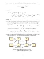
Figure 22.1. Evolution of the Finite Element Method.

“Astonishing success”, however, carries its own dangers. By the early 1980s the FEM began to be
regarded as “mature technology” by US funding agencies. By now that feeling has hardened to the point
that it is virtually impossible to get significant research support for fundamental work in FEM. This
viewpoint has been reinforced by major software developers, which proclaim their products as solutions
to all user needs.
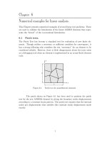
Is this perception correct? It certainly applies to the core FEM, or orthodox FEM. This is the material
taught in textbooks and which is implemented in major software products. Core FEM follows what may
be called the Ritz-Galerkin and Direct Stiffness Method canon. Beyond the core there is an evolving
FEM. This is strongly rooted on the core but goes beyond textbooks. Finally there is a frontier FEM,
which makes only partial or spotty use of core knowledge. See Figure 22.1.
By definition core FEM is mature. As time goes, it captures segments of the evolving FEM. For example,
most of the topic of FEM mesh adaptivity can be classified as evolving, but will eventually become part
of the core. Frontier FEM, on the other hand, can evolve unpredictably. Some components prosper,
mature and eventually join the core, some survive but never become orthodox, while others wither and
die.
Four brilliant contributions of Bruce Irons, all of which were frontier material when first published, can
be cited as examples of the three outcomes. Isoparametric elements and frontal solvers rapidly became
integral part of the core technology. The patch test has not become part of the core, but survives as a
useful if controversial tool for element development and testing. The semi-loof shell elements quietly
disappeared.
Topics that drive frontier FEM include multiphysics, multiscale models, symbolic and high performance
computation, integrated design and manufacturing, advances in information technology, optimization,

inverse problems, materials, treatment of joints and interfaces, and high performance elements. This
paper deals with the last topic.
§22.2. HIGH PERFORMANCE ELEMENTS
An important area of frontier FEM is the construction of high performance (HP) finite elements. These
22–4


22–5

§22.2

HIGH PERFORMANCE ELEMENTS

were defined by Felippa and Militello [10] as “simple elements that deliver engineering accuracy with
arbitrary coarse meshes.” Some of these terms require clarification.
Simple means the simplest geometry and freedom configuration that fits the problem and target accuracy
consistent with human and computer resources. This can be summed up in one FEM modeling rule: use
the simplest element that will do the job.
Engineering accuracy is that generally expected in most FEM applications in Aerospace, Civil and
Mechanical Engineering. Typically this is 1% in displacements and 10% in strains, stresses and derived
quantities. Some applications, notably in Aerospace, require higher precision in quantities such as natural
frequencies, shape tolerances, or in long-time simulations.
Coarse mesh is one that suffices to capture the important physics in terms of geometry, material and load
properties. It does not imply few elements. For example, a coarse mesh for a fighter aircraft undergoing
maneuvers may require several million elements. For simple benchmark problems such as a uniformly
loaded square plate, a mesh of 4 or 16 elements may be classified as coarse.
Finally, arbitrary mesh implies low sensitivity to skewness and distortion. This attribute is becoming
important as push-button mesh generators gain importance, because generated meshes can be of low
quality compared to those produced by an experienced analyst.
For practical reasons we are interested only in the construction of HP elements with displacement nodal

degrees of freedom. Such elements are characterized by their stiffness equations, and thus can be plugged
into any standard finite element program.
§22.2.1. Tools for Construction of HP Elements
The origins of HP finite elements may be traced to several investigators in the late 1960s and early
1970s. Notable early contributions are those of Clough, Irons, Taylor, Wilson and their coworkers. The
construction techniques made use of incompatible shape functions, the patch test, reduced, selective and
directional integration. These can be collectively categorized as unorthodox, and in fact were labeled as
“variational crimes” at that time by Strang and Fix [4].
A more conventional development, pioneered by Pian, Tong and coworkers, made use of mixed and
hybrid variational principles. They developed elements using stress or partial stress assumptions, but the
end product were standard displacement elements. These techniques were further refined in the 1980s.
A good expository summary is provided in the book by Zienkiewicz and Taylor [11].
New innovative approaches came into existence in the 1980s. The most notable have been the Free
Formulation of Bergan and Nyg˚ard [12,13], and the Assumed Strain method pioneered by MacNeal
[14]. The latter was further developed along different paths by Bathe and Dvorkin [15], Park and Stanley
[16], and Simo and Hughes [17].
§22.2.2. Unification by Parametrized Variational Principles
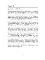
The approach taken by the author started from collaborative work with Bergan in Free Formulation (FF)
high performance elements. The results of this collaboration were a membrane triangle with drilling
freedoms described in Bergan and Felippa [18] and a plate bending triangle presented by Felippa and
Bergan [19]. It continued with exploratory work using the Assumed Natural Strain (ANS) method
of Park and Stanley [16]. Eventually FF and ANS coalesced in a variant of ANS called Assumed
Natural Deviatoric Strain, or ANDES. High performance elements based on the ANDES formulation
are described by Militello and Felippa [20] and Felippa and Militello [21].
22–5


Chapter 22: RECENT ADVANCES IN FINITE ELEMENT TEMPLATES

FF:

ANS:

Free Formulation
o

Bergan & Hanssen 1975, Bergan & Nygard 1984

Fundamental decomposition K = K b + Kh
Kb is constant stress hybrid (1985)
K h is derivable from a one parameter
stress-displacement hybrid principle (1987)

22–6

Assumed Natural Strain Formulations

MacNeal 1978, Bathe & Dvorkin 1985, Park & Stanley 1986

Strain-displacement variational principle,
equivalence with incompatible elements (1988)
Parametrized deviatoric strain produces K h
(1989)

ANDES Formulation (1990)

GENERAL PARAMETRIZED VARIATIONAL PRINCIPLES (1990)

Pattern and invariance recognition (1993)

Multiple parameter elements (1991)

TEMPLATES (1994)

Figure 22.2. The road to templates.

This unification work led naturally to a formulation of elasticity functionals containing free parameters.
These were called parametrized variational principles, or PVPs in short. Setting the parameters to specific
numerical values produced the classical functionals of elasticity such as Total Potential Energy, HellingerReissner and Hu-Washizu. For linear elasticity, three free parameters in a three-field functional with
independently varied displacements, strains and stresses are sufficient to embed all classical functionals.
Two survey articles with references to the original papers are available [22,23].
One result from the PVP formulation is that, upon FEM discretization, free parameters appear at the
element level. One thus naturally obtains families of elements. Setting the free parameters to numerical
values produces specific elements. Although the PVP Euler-Lagrange equations are the same excepts
for weights, the discrete solution produced by different elements are not. Thus an obvious question
arises: which free parameters produce the best elements? It turns out that there is no clear answer to
the question, because the best set of parameters depends on the element geometry. Hence the equivalent
question: which is the best variational principle? makes no sense.
The PVP formulation led, however, to an unexpected discovery. The configuration of elements constructed according to PVPs and the usual assumptions on displacements, stresses and strains was observed to follow specific algebraic rules. Such configurations could be parametrized directly without
going through the source PVP. This observation led to a general formulation of finite elements as templates.
The aforementioned developments are flowcharted in Figure 22.2.
§22.3. FINITE ELEMENT TEMPLATES
A finite element template, or simply template, is an algebraic form that represents element-level stiffness
equations, and which fulfills the following conditions:
(C) Consistency: the Individual Element Test (IET) form of the patch test, introduced by Bergan and
Hanssen [24], is passed for any element geometry.
22–6


22–7

§22.3

w1

FINITE ELEMENT TEMPLATES

z,w
EI = constant

w2

θ1
L
θ2
One free parameter
0

0 0 0 

EI 
 0 1 0 −1  + β E I
K = Kb + K h =
L 0 0 0 0 
L3
0 −1 0 1

x

 4

−2L
 −4
−2L

−2L
L2
2L
L2

−4
2L
4
2L

−2L 
L2 

2L
2
L

Figure 22.3. Template for Bernoulli-Euler prismatic plane beam.

(S) Stability: the stiffness matrix satisfies correct rank and nonnegativity conditions.
(P) Parametrization: the element stiffness equations contain free parameters.
(I) Invariance: the element equations are observer invariant. In particular, they are independent of node
numbering and choice of reference systems.
The first two conditions: (C) and (S), are imposed to ensure convergence. Property (P) permits performance optimization as well as tuning elements to specific needs. Property (I) helps predictability and
benchmark testing.
Setting the free parameters to numeric values yields specific element instances.

§22.3.1. The Fundamental Decomposition
A stiffness matrix derived through the template approach has the fundamental decomposition
K = Kb (αi ) + Kh (β j )

(22.1)

Here Kb and Kh are the basic and higher-order stiffness matrices, respectively. The basic stiffness matrix
Kb is constructed for consistency and mixability, whereas the higher order stiffness Kh is constructed
for stability (meaning rank sufficiency and nonnegativity) and accuracy. As further discussed below, the
higher order stiffness Kh must be orthogonal to all rigid-body and constant-strain (curvature) modes.
In general both matrices contain free parameters. The number of parameters αi in the basic stiffness is
typically small for simple elements. For example, in the 3-node, 9-DOF KPT elements considered here
there is only one basic parameter, called α. This number must be the same for all elements in a mesh to
insure satisfaction of the IET [18].
On the other hand, the number of higher order parameters β j can be in principle infinite if certain
components of Kh can be represented as a polynomial series of element geometrical invariants. In
practice, however, such series are truncated, leading to a finite number of β j parameters. Although the
β j may vary from element to element without impairing convergence, often the same parameters are
retained for all elements.
22–7


Chapter 22: RECENT ADVANCES IN FINITE ELEMENT TEMPLATES

22–8

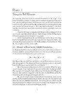
As an illustration Figure 22.3 displays the template of a simple one-dimensional element: a 2-node,
4-DOF plane Bernoulli-Euler prismatic beam. This has only one free parameter: β, which scales the
higher order stiffness. A simple calculation [22] shows that its optimal value is β = 3, which yields the
well-known Hermitian beam stiffness. This is known as a universal template since it include all possible

beam elements that satisfy the foregoing conditions.
§22.3.2. Constructing the Component Stiffness Matrices
The basic stiffness that satisfies condition (C) is the same for any formulation. It is simply a constant
stress hybrid element [13,18]. For a specific element and freedom configuration, Kb can be constructed
once and for all.
The formulation of the higher order stiffness Kh is not so clear-cut, as can be expected because of the
larger number of free parameters. It can be done by a variety of techniques, which are summarized in
a article by Felippa, Haugen and Militello [25]. Of these, one has proven exceedingly useful for the
construction of templates: the ANDES formulation. ANDES stands for Assumed Natural DEviatoric
Strains. It is based on assuming natural strains for the high order stiffness. For plate bending (as well as
beams and shells) natural curvatures take the place of strains.
Second in usefulness is the Assumed Natural DEviatoric STRESSes or ANDESTRESS formulation,
which for bending elements reduces to assuming deviatoric moments. This technique, which leads to
stiffness templates that contain inverses of natural flexibilities, is not considered here.
§22.3.3. Basic Stiffness Properties
The following properties of the template stiffness equations are collected here for further use. They
are discussed in more detail in the article by Felippa, Haugen and Militello [25]. Consider a test
displacement field, which for thin plate bending will be a continuous transverse displacement mode
w(x, y). [In practical computations this will be a polynomial in x and y.] Evaluate this at the nodes to
form the element node displacements u. These can be decomposed into
u = ub + uh = ur + uc + uh ,

(22.2)

where ur , uc and uh are rigid body, constant strain and higher order components, respectively, of u.
The first two are collectively identified as the basic component ub . The matrices (22.1) must satisfy the
stiffness orthogonality conditions
Kb ur = 0,

Kh ur = 0,

K h uc = 0

(22.3)

while Kb represents exactly the response to uc .
The strain energy taken up by the element under application of u is U = 12 uT Ku. Decomposing K and
u as per (22.1) and (22.2), respectively, and enforcing (22.3) yields
U = 12 (ub + uh )T Kb (ub + uh ) + 12 uhT Kh uh = Ub + Uh

(22.4)

Ub and Uh are called the basic and higher order energy, respectively. Let Uex be the exact energy taken
up by the element as a continuum body subjected to the test displacement field. The element energy
ratios are defined as
U
Ub
Uh
ρ=
= ρb + ρ h , ρ b =
, ρh =
.
(22.5)
Uex
Uex
Uex
Here ρb and ρh are called the basic and higher order energy ratios, respectively. If uh = 0, ρ = ρb = 1
because the element must respond exactly to any basic mode by construction. For a general displacement
mode in which uh does not vanish, ρb is a function of the αi whereas ρh is a function of the β j .
22–8

22–9

§22.4

TEMPLATES FOR 3-NODE KPT ELEMENTS

;;;;
;;;;
uz

θy

θx
K = K b (α i) + Kh (β j )
Template
name
KPT-1-9 element-acronym α β10 β20 β30 β40 β50 β60 β70 β80 β90
Template

element-acronym α
KPT-1-36

β10
β11
β12
β13

β20

β21
β22
β23

β30
β31
β32
β33

β40
β41
β42
β43

β50
β51
β52
β53

β60
β61
β62
β63

β70
β71
β72
β73

β80

β81
β82
β83

β90 signatures
β92
β93
β93

Figure 22.4. Template for Kirchhoff plate-bending triangles (KPT) studied here.

§22.3.4. Constructing Optimal Elements
By making a template sufficiently general all published finite elements for a specific configuration can
be generated. This includes those derivable by orthodox techniques (for example, shape functions) and
those that are not. Furthermore, an infinite number of new elements arise. The same question previously
posed for PVPs arises: Can one select the free parameters to produce an optimal element?
The answer is not yet known for general elements. The main unresolved difficulty is: which optimality
conditions must be imposed at the local (element) level? While some of them are obvious, for example
those requiring observer invariance, most of the others are not. The problem is that a detailed connection between local and global optimality is not fully resolved by conventional FEM error analysis.
Such analysis can only provide convergence rates expressed as C h m in some error norm, where h is a
characteristic mesh dimension and m is usually the same for all template instances. The key to high
performance is the coefficient C, but this is problem dependent. Consequently, verification benchmarks
are still inevitable.
As noted, conventional error analysis is of limited value because it only provides the exponent m,
which is typically the same for all elements in a template. It follows that several template optimization
constraints discussed later are heuristic. But even if the local-to-global connection were fully resolved, a
second technical difficulty arises: the actual construction and optimization of templates poses formidable
problems in symbolic matrix manipulation, because one has to carry along arbitrary geometries, materials
and free parameters.
Until recently those manipulations were beyond the scope of computer algebra systems (CAS) for all

but the simplest elements. As personal computers and workstations gain in CPU speed and storage, it
is gradually becoming possible to process two-dimensional elements for plane stress and plate bending.
Most three-dimensional and curved-shell elements, however, still lie beyond the power of present systems.
Practitioners of optimization are familiar with the dangers of excessive perfection. A system tuned
to operate optimally for a narrow set of conditions often degrades rapidly under deviation from such
conditions. The benchmarks of Section 8 show that a similar difficulty exists in the construction of
optimal plate elements, and that expectations of an “element for all seasons” must be tempered.
22–9


22–10

Chapter 22: RECENT ADVANCES IN FINITE ELEMENT TEMPLATES

§22.4. TEMPLATES FOR 3-NODE KPT ELEMENTS
The application of the template approach is rendered specific by studying a particular configuration:
a 3-node flat triangular element to model bending of Kirchhoff (thin) plates. The element has the
conventional 3 degrees of freedom: one transverse displacement and three rotations at each corner, as
illustrated in Figure 22.4.
For brevity this will be referred to as a Kirchhoff Plate Triangle, or KPT, in the sequel. The complete
development of the template is given in the Appendix. In the following sections we summarize only the
important results necessary for the application of local optimality constraints.
§22.4.1. Stiffness Decomposition
For the KPT elements under study the configuration of the stiffness matrices in (22.1) can be shown in
more detail. Assuming that the 3 × 3 moment-curvature plate constitutive matrix D is constant over the
triangle, we have
Kb =

1
LDLT ,

A

Kh =

A T
T
Bχ4 Dχ Bχ 4 + BχT 5 Dχ Bχ 5 + Bχ6
Dχ Bχ6 .
3

(22.6)

Here A is the triangle area, L is the 9×3 force lumping matrix that transforms a constant internal moment
field to node forces, Bχm are 3 × 9 matrices relating natural curvatures at triangle midpoints m = 4, 5, 6
to node displacements, and Dχ is the plate constitutive matrix transformed to relate natural curvatures
to natural moments. Parameter α appears in L whereas parameters β j appear in Bχm . Full expressions
of these matrices are given in the Appendix.
§22.4.2. The KPT-1-36 and KPT-1-9 Templates
A useful KPT template is based on a 36-parameter representation of Kh in which the series noted above
retains up to the linear terms in three triangle geometric invariants λ1 , λ2 and λ3 , defined in the Appendix,
which characterize the deviations from the equilateral-triangle shape. The template is said to be of order
one in the λs. It has a total of 37 free parameters: one α and 36 βs. Collectively this template is identified
as KPT-1-36. Instances are displayed using the following tabular arrangement:
acronym

α

β10
β11
β12

β13

β20
β21
β22
β23

β30
β31
β32
β33

β40
β41
β42
β43

β50
β51
β52
β53

β60
β61
β62
β63

β70
β71
β72

β73

β80
β81
β82
β83

β90
β91
β92
β93

/βsc

(22.7)

Here βsc is a scaling factor by which all displayed βi j must be divided; e.g. in the DKT element listed
in Table 22.1 β10 = −6/4 = −3/2 and β41 = 4/4 = 1. If βsc is omitted it is assumed to be one.
Setting the 37 parameters to numeric values yield specific elements, identified by the acronym displayed
on the left. Some instances that are interesting on account of practical or historical reasons are collected
in Table 22.1. Collectively these represents a tiny subset of the number of published KPT elements,
which probably ranges in the hundreds, and is admittedly biased in favor of elements developed by
the writer and colleagues. Table 22.2 identifies the acronyms of Table 22.1 correlated with original
publications where appropriate.
An interesting subclass of (22.7) is that in which the bottom 3 rows vanish: β11 = β12 = . . . β93 = 0.
This 10-parameter template is said to be of order zero because the invariants λ1 , λ2 and λ3 do not appear
22–10


22–11

§22.4

TEMPLATES FOR 3-NODE KPT ELEMENTS

Table 22.1. Template Signatures of Some Existing KPT Elements
Acronym
ALR

α
0

AQR0
AQRBE
AQR1

0√
1/ 2
1

AVG
BCIZ0
BCIZ1

0
0
1

DKT

1

FF0
FF1
HCT

0
1
1

β1 j β2 j β3 j β4 j β5 j
−3 0
0
0
0
−6 0
0
0
0
0
0
0
0
0
0
0
0
0
0
Same βs as AQR1

Same βs as AQR1
−3 0
0
0
0
−2 0
0
0
0
0
0
0
0
0
0
0
0
0
0
−3 0
0
0
0
−3 1
1
0
0
−3 0
0 −1 1
0

0
0
2
0
0
0 −2 0
0
0
2
0
0
2
−6 1
1 −2 2
0
0
0
4
0
0
0
2
0
0
0 −2 0
0
4
−9 1
1 −2 2
Same βs as FF0.

−11 5
0 −2 2
6
0
0
4
0
0
0 20
0
0
0
10 0
0
4

β6 j
0
0
0
0

β7 j β8 j β9 j
0
3
0
0
0
0
0

0
0
0 −6 0

βsc
/2

0
0
0
0
0
−1
0
0
−2
0
−1
0
2
0
−1

0
3
0
0
0
0
0

0 −4
0 −2 0
0
3
0
−1 3
0
0
3
0
2
0
0
0
0
0
0
0
0
−1 6
0
−2 0
0
0
0
0
0
0
0
−1 9

0

/2

0
0
20
0

−5 11
10 0
0
0
0
6

0
0
0
0

/2
/2
/2

/4

/6
/4

in the higher order stiffness. It is identified as KPT-1-9. For brevity it will be written simply as
acronym

α

β10 β20 β30

β40 β50 β60

β70 β80 β90

/βsc

(22.8)

omitting the zero entries.
§22.4.3. Element Families
Specializations of (22.7) and (22.8) that still contain free parameters are called element families. In
such a case the free parameters are usually written as arguments of the acronym. For example, Table
22.4 defines the ARI, or Aspect Ratio Insensitive, family derived in Section 6. ARI has seven free
parameters identified as α, β10 , β20 , β30 , γ0 , γ1 and γ2 . Consequently the template acronym is written
ARI(α, β10 , β20 , β30 , γ0 , γ1 , γ2 ).
A family whose only free parameter is α is called an α-family. Its instances are called α-variants. In
some α families the β coefficients are fixed. For example in the AQR(α) and FF(α) families only α
changes. Some practically important instances of those families are shown in Table 22.1. In other
α-families the βs are functions of α. For example this happens in the BCIZ(α) family, two instances of
which, obtained by setting α = 0 and α = 1, are shown on Table 22.1.
§22.4.4. Template Genetics: Signatures and Clones
22–11

Chapter 22: RECENT ADVANCES IN FINITE ELEMENT TEMPLATES

22–12

Table 22.2. Element Identifiers Used in Table 22.1
Acronym Description
ALR

Assumed Linear Rotation KPT element of Militello and Felippa [20].

AQR1

Assumed Quadratic Rotation KPT element of Militello and Felippa [20].

AQR0

α-variant of AQR1 with α = 0.

AVG

Average curvature KPT element of Militello and Felippa [20].

BCIZ0

Nonconforming element of Bazeley, Cheung, Irons and Zienkiewicz [26]
“sanitized” with α = 0 as described by Felippa, Haugen and
Militello [25]. Historically the first polynomial-based, complete,
nonconforming KPT and the motivation for the original (multielement)
patch test of Irons. See Section 4.4 for two clones of BCIZ0.

BCIZ1

Variant of above, in which the original BCIZ is sanitized with α = 1.

DKT

Discrete Kirchhoff Triangle of Stricklin et al. [30]
streamlined by Batoz [31]; see also Bathe, Batoz and Ho [32]

FF0

Free Formulation element of Felippa and Bergan [19].

FF1
HCT

α variant of FF0 with α = 1.
Hsieh-Clough-Tocher element presented by Clough and Tocher [33]
with curvature field collocated at the 3 midpoints. The original
(macroelement) version was the first successful C 1 conforming KPT.

√
AQRBE α-variant of AQR1 with α = 1/ 2; of interest because it is BME.

An examination of Table 22.1 should convince the reader that template coefficients uniquely define an
element once and for all, although the use of author-assigned acronyms is common in the FE literature.
The parameter set can be likened to an “element genetic fingerprint” or “element DNA” that makes it a
unique object. This set is called the element signature.
If signatures were randomly generated, the number of element instances would be of course huge:

more precisely ∞37 for 37 parameters. But in practice elements are not fabricated at random. Attractors
emerge. Some element derivation methods, notably those based on displacement shape functions, tend to
“hit” certain signature patterns. The consequence is that the same element may be discovered separately
by different authors, often using dissimilar derivation techniques. Such elements will be called clones.
Cloning seems to be more prevalent among instances of the order-zero KPT-1-9 template (22.8). Some
examples discovered in the course of this study are reported.
The first successful nonconforming triangular plate bending element was the original BCIZ [26]. This
element, however, does not pass the Individual Element Test (IET), and in fact fails Irons’ original patch
test for arbitrary mesh patterns. The source of the disease is the basic stiffness. The element can be
“sanitized” by removing the infected matrix as described by Felippa, Haugen and Militello [25]. This
is replaced by a healthy Kb with, for example, α = 0 or α = 1. This transplant operation yields the
elements called BCIZ0 and BCIZ1, respectively, in Table 22.1. [These are two instances of the BCIZ(α)
family.] Note that BCIZ0 pertains to the KPT-1-9 template.
In the 3rd MAFELAP Conference, Hanssen, Bergan and Syversten [27] reported a nonconforming
element which passed the IET and (for the time) was of competitive performance. Construction of its
template signature revealed it to be a clone of BCIZ0. The plate bending part of the TRIC shell element
22–12


22–13

§22.4

TEMPLATES FOR 3-NODE KPT ELEMENTS

ARI2:

Table 22.3 - Linear Constraints for KPT-1-36 Template
β11 = (2β10 + β20 + 3β30 − 4β40 )/3, β22 = (8β20 − 4β30 + 2β40 )/9

ARI1:
ARI1:
ARI1:

β33 = β20 − β30 − β22 , β92 = 2β10 + β20 + 3β30 − 4β40 − β11
β23 = −2β20 + β22 , β32 = 2β30 + β33 , β41 = −2β40 − β33
β12 = β22 , β93 = β33 , β13 = −β33 , β82 = β22 , β43 = −β33

ARI0:

β21 = β31 = β42 = β52 = β63 = β73 = 0

ENO1:

β32 = β23 +β41 , β92 = 2β11 −β12 +β82 , β13 = β93 −β82 , β33 = β22 +β43

ENO0:

β40 = −β20 − β30

OI1:
OI1:
OI1:

β51 = β52 + β43 − β42 , β53 = β52 − β42 + β41 , β61 = β63 − β31 + β33 ,
β62 = β63 + β32 − β31 , β71 = β73 − β21 + β23 , β72 = β73 − β21 + β22 ,
β81 = β82 − β12 + β13 , β83 = β82 − β12 + β11 , β91 = β93

OI0:

β50 = −β40 ,

β80 = −β10 ,

β60 = −β30 ,

β70 = −β20 ,

β90 = 0

[28] is also a clone of BCIZ0.
An energy orthogonal version of the HBS element was constructed by Nyg˚ard in his Ph.D. thesis [29].
Its signature turned out to agree with that of the FF0 element, constructed by Felippa and Bergan [19]
with a different set of higher order shape functions.
Clones seem rarer in the realm of the full KPT-1-36 template because of its greater richness. The DKT
[30–32] appears to be an exception. Although this popular element is usually constructed by assuming
rotation fields, it coalesced with one of the ANDES elements derived by Militello and Felippa [20] by
assuming natural deviatoric curvatures. At the time the coalescence was suspected from benchmarks, and
later verified by direct examination of stiffness matrices. Using the template formulation such numerical
tests can be bypassed, since it is sufficient to compare signatures.
§22.4.5. Parameter Constraints
To construct element families and in the limit, specific elements, constraints on the free parameters must
be imposed. One key difficulty, already noted in Section 3.4, emerges. Constraints must be imposed
at the local level of either an individual element or simple mesh units, but they should lead to high
performance behavior at the global level. There is as yet no mathematical framework for establishing
those connections.
Several constraint types have been used in this and previous work: (1) invariance, (2) skewness and aspect
ratio insensitivity, (3) distortion insensitivity, (4) truncation error minimization, (5) energy balance, (6)
energy orthogonality, (7) morphing, (8) mesh direction insensitivity. Whereas (1) and (2) have clear
physical significance, the effect of the others has to be studied empirically on benchmark problems.

Conditions that have produced satisfactory results are discussed below with reference to the KPT template.
The reader should be cautioned, however, that these may not represent the final word inasmuch as
templates are presently a frontier subject. For convenience the constraints can be divided into linear and
nonlinear, the former being independent of constitutive properties.
§22.4.6. Staged Element Design
Taking an existing KPT element that passes the IET and finding its template signature is relatively
straightforward with the help of a computer algebra program. Those listed in Table 22.1 were obtained
using Mathematica. But in element design we are interested in the reverse process: starting from a general
22–13


Chapter 22: RECENT ADVANCES IN FINITE ELEMENT TEMPLATES

Configuration (A)

L /r

y

r

ψ

x

Configurations (B,C)

22–14

L

ξL

(1−ξ) L
(B): H = r L

y

r

(C): H = L/r
x

L

Figure 22.5. Triangle configurations for the study of ARI constraints.

template such as KPT-1-36, to arrive at specific elements that display certain desirable characteristics.
Experience shows that this is best done in two stages.
First, linear constraints on the free parameters are applied to generate element families. The dependence
on the remaining free parameters is still linear.
Second, selected energy balance constraints are imposed. For linear elastic elements such constraints
are quadratic in nature. Consequently there is no guarantee that real solutions exist. If they do, solutions
typically produce families with few (usually 1 or 2) free parameters; in particular α families. Finally,
setting the remaining parameters to specific values produces element instances.
§22.5. LINEAR CONSTRAINTS
Three types of linear constraints have been used to generate element families.
§22.5.1. Observer Invariance (OI) Constraints
These pertain to observer invariance. If the element geometry exhibits symmetries, those must be
reflected in the stiffness equations. For example, if the triangle becomes equilateral or isoceles, certain

equality conditions between entries of the curvature-displacement matrices must hold. The resulting
constraints are linear in the βs.
For the KPT-1-36 template one obtains the 14 constraints labeled as OI0 and OI1 in Table 22.3. The
five OI0 constraints pertain to the order zero parameters and would be the only ones applicable to the
KPT-1-9 template. They can be obtained by considering an equilateral triangle. The nine OI1 constraints
link parameters of order one. This constraint set must be the first imposed and applies to any element.
§22.5.2. Aspect Ratio Insensitivity (ARI) Constraints
A second set of constraints can be found by requiring that the element be aspect ratio insensitive, or
22–14


22–15

§22.5

LINEAR CONSTRAINTS

ARI for short, when subjected to arbitrary node displacements. A triangle that violates this requirement
becomes infinitely stiff for certain geometries when a certain dimension aspect ratio r goes to infinite.
To express this mathematically, it is sufficient to consider the triangle configurations (A,B,C) depicted in
Figure 22.5. In all cases L denotes a triangle dimension kept fixed while the aspect ratio r is increased.
In configuration A, the angle ψ is kept fixed as r → ∞. The opposite angles tend to zero and π/2 − ψ.
The case ψ = 90◦ = π/2 is particularly important as discussed later. In configurations (B) and (C) the
ratio ξ is kept fixed as r → ∞, and angles tend to π, π/2 or zero.
As higher order test displacements we select the four cubic modes w30 = x 3 , w21 = x 2 y, w12 = x y 2 and
w03 = y 3 . Any other cubic mode is a combination of those four. Construct the element energy ratios
defined by Equation (22.5). The important dependence of those ratios on physical properties and free
parameters is
ρ = ρbm (r, ψ, α) + ρhm (r, ψ, β j )
(22.9)

where m = 30, 21, 12, 03 identifies modes x 3 , x 2 y, x y 2 and y 3 , respectively. (The dependence on
L and constitutive matrix D is innocuous for this study and omitted for simplicity). Take a particular
configuration (A,B,C) and mode m, and let r → ∞. If ρ remains nonzero and bounded the element is
said to be aspect ratio insensitive for that combination. If ρ → ∞ the element is said to experience
aspect ratio locking, whereas if ρ → 0 the element becomes infinitely flexible. If ρ remains nonzero
and bounded for all modes and configurations the element is called completely aspect ratio insensitive.
The question is whether free parameters can be chosen to attain this goal.
As posed an answer appears difficult because the ratios (22.9) are quadratic in the free parameters, rational
in r , and trascendental in ψ. Fortunately the question can be reduced to looking at the dependence of the
curvature-displacement matrices on r as r → ∞. Entries of these matrices are linear functions of the
free parameters. As r → ∞ no entry must grow faster than r , because exact curvatures grow as O(r ).
For example, if an entry grows as r 2 , setting its coefficient to zero provides a linear constraint from
which the dependence on L and ψ is factored out. The material properties do not come in. Even with
this substantial simplification the use of a CAS is mandatory to handle the elaborate symbolic algebra
involved, which involves the Laurent expansion of all curvature matrices. The result of the investigation
for the KPT-1-36 template can be summarized as follows.
(1) The basic energy ratio ρb is bounded for all ψ and all m in configuration (A). In configurations (B)
and (C) it is unbounded as O(r ) in two cases: m = 30 if α = 1, and m = 21 for any α.
(2) The higher order energy ratio ρh can be made bounded for all ψ and m by imposing the 18 linear
constraints listed in Table 22.3 under the ARI label.
(3) The foregoing bound on ρh is not possible for the KPT-1-9 template. Thus a signature of the form
(22.8) is undesirable from a ARI standpoint.
Because of the basic stiffness shortcoming noted in (1), a completely ARI element cannot be constructed.
However, the βs can be selected to guarantee that ρh is always bounded. The resulting constraints are
listed in Table 22.3. They are grouped in three subsets labeled ARI0, ARI1 and ARI2.
Subset ARI0 requires β21 = β31 = β42 = β52 = β63 = β73 = 0. If any of these 6 parameters is nonzero,
one or more entries of the deviatoric curvature displacement matrices grow as r 3 in the 3 configurations.
This represents disastrous aspect ratio locking and renders any such element useless.
Once OI0, OI1 and ARI0 are imposed, subset ARI1 groups 10 constraints obtained by setting to zero
O(r 2 ) grow in configuration (A) for all HO modes. This insures that ρ = ρb + ρh stays bounded in that

configuration (because ρb stays bounded for any α). In Table 22.3 they are listed in reverse order of that
found by the symbolic analysis program, which means that the most important ones appear at the end.
22–15


22–16

Chapter 22: RECENT ADVANCES IN FINITE ELEMENT TEMPLATES

Table 22.4. Three Element Families Derivable From KPT-1-36
ARI(α,β10 ,β20 ,β30 ,γ0 ,γ1 ,γ2 )

α

β10
β11
β22

β20 β30
0

0

β22 β62

β40

−β40 −β30 −β20 −β10

β41

−β61

β61

β71

0

0

β62

β22

β22

β92

β41

0

0

β11

β61

−β61 β71 β61 −β61

0

−β61 β61

where β40 = −β20 − β30 + γ0 , β11 = (2β10 + β20 + 3β30 − 4β40 )/3 + γ1 ,
β22 = (8β20 − 4β30 + 2β40 )/9 + γ2 , β61 = β20 − β22 − β30 , β41 = −β61 − 2β40 ,
β62 = β20 − β22 + β30 , β71 = −2β20 + β22 and β92 = 2β10 − β11 + β20 + 3β30 − 4β40 .
ENO(α, β10 , β20 , β30 , β11 , β41 ,
β12 , β22 , β82 , β23 , β43 , β93 )

α

β10
β11

β20 β30
0

0

β40

−β40 −β30 −β20 −β10

0

β41

β43

β33

β23

β81

β93

β12

β22 β32

0

0

β32

β22

β82

β92

β13

β23 β33

β43

β41

0

0

β83

β93

where β40 = −β20 − β30 , β81 = −β12 + β93 , β32 = β23 + β41 , β92 = 2β11 − β12 + β82 ,
β13 = −β82 + β93 , β33 = β22 + β43 and β83 = β11 − β12 + β82 .
ARIENO(α, β10 , β20 , β30 )

ARI(α, β10 , β20 , β30 , 0, 0, 0)

Once OI0, OI1 and ARI0 and ARI1 are imposed, the 2-constraint subset ARI2 guarantees that ρh is
bounded for configurations (B) and (C). Since ρb is not necessarily bounded in this case, these conditions
have minor practical importance.
Imposing OI0, OI1, ARI0 and ARI1 leaves 37 − 5 − 9 − 6 − 10 = 7 free parameters, and produces the
so-called ARI family defined in Table 22.4. Of the seven parameters, four are chosen to be the actual
template parameters α, β10 , β20 , and β30 . Three auxiliary parameters, called γ1 , γ2 and γ3 , are chosen to
complete the generation of the ARI family as defined in Table 22.4.
This family is interesting in that it includes all existing high-performance elements, such as DKT and
AQR1, as well as some new ones developed in the course of this study.
§22.5.3. Energy Orthogonality (ENO) Constraints
Energy orthogonality (ENO) means that the average value of deviatoric strains over the element is zero.
Mathematically, Bχ4 + Bχ5 + Bχ 6 = 0. This condition was a key part of the early developments of the
Free Formulation by Bergan [12] and Bergan and Nyg˚ard [13], as well as of HP elements developed

during the late 1980s and early 1990s.
The heuristic rationale behind ENO is to limit or preclude energy coupling between constant strain and
higher order modes. A similar idea lurks behind the so-called “B-bar” formulation, which has a long
and checkered history in modeling incompressibility and plastic flow.
For the KPT-1-36 element one may start with the OI0 and OI1 constraints as well as ARI0 (to preclude catastrophic locking), but ignoring ARI1 and ARI2. Then the ENO condition leads to the linear
constraints labeled as ENO0 and ENO1 in Table 22.3. These group conditions on the order zero and
one parameters, respectively. Imposing OI0, OI1, ARI0, ENO0 and ENO1 leads to the ENO family
defined in Table 22.4, which has 12 free parameters. Elements ALR, FF0 and FF1 of Table 22.1 can
be presented as instance of this family as shown later in a “genealogy” Table.
22–16


22–17

§22.6

QUADRATIC CONSTRAINTS

If instead one starts from the ARI family it can be verified that ENO is obtained if γ0 = γ1 = γ2 = 0; that
is, only three constraints are needed instead of five. [This is precisely the rationale for selecting those
“ENO deviations” as free arguments]. Moreover, the order-one constraints γ1 = γ2 = 0 are precisely
ARI2 in disguise.
Setting γ0 = γ1 = γ2 = 0 in ARI yields a four-parameter family called ARIENO (pronounced like the
French “Arienne”). The free parameters are α, β10 , β20 and β30 . Its template is defined in Table 22.4.
As noted, this family incorporates all constraints listed in Table 22.3. (These add up to 37 relations, but
there are 4 redundancies.)
As noted all HP elements found to date are ARI (ALR, FF0 and FF1 are not considered HP elements
now). Most are ENO, but there are some that are not. One example is HCTS, a “smoothed HCT” element
developed in this study. Hence circumstantial evidence suggests that ARI is more important than ENO.
In the present investigation ENO is used as a guiding principle rather than an a priori constraint.

§22.6. QUADRATIC CONSTRAINTS
As noted in the foregoing section, the ARI family — and its ARIENO subset — is a promising source of
high performance KPT elements. But seven parameters remain to be set to meet additional conditions.
These fall into the general class of energy balance constraints introduced in [18]. Unit energy ratios
are imposed for specific mesh unit geometries, loadings and boundary conditions. Common feature of
such constraints, for linear elements, are: they involve constitutive properties, and they are quadratic in
the free parameters. Consequently real parameter solutions are not guaranteed. Even if they have real
solutions, the resulting families may exist only for limited parameter ranges.
Numerous variants of the energy balance tests have been developed over the years. Because of space
constraints only three variations under study are described below. All of them have immediate physical
interpretation in terms of the design of custom elements. They have been applied assuming isotropic
material with zero Poisson’s ratio.
§22.6.1. Morphing Constraints
This is a class of constraints that is presently being studied to ascertain whether enforcement would
be generally beneficial to element performance. Consider the two-KPT-element rectangular mesh unit
shown in Figure 22.6. The aspect ratio r is the ratio of the longest rectangle dimension L to the width
b = L/r . The plate is fabricated of a homogeneous isotropic material with zero Poisson’s ratio and
thickness t. Axis x is selected along the longitudinal direction. We study the two morphing processes
depicted at the top of Figure 22.6. In both the aspect ratio r is made to increase, but with different
objectives.
Plane Beam Limit. The width b = L/r is decreased while keeping L and t fixed. The limit is the thin,
Bernoulli-Euler plane beam member of rectangular cross section t × b, b << t, shown at the end of
the beam-morphing arrow in Figure 22.6. This member can carry exactly a linearly-varying bending
moment M(x) and a constant transverse shear V , although shear deformations are not considered.
Twib Limit. Again the width b = L/r is decreased by making r grow. The thickness t, however, is still
considered small with respect to b. The limit is the twisted-ribbon member of cross section t ×b, t << b,
shown on the left of Figure 22.6. This member, called a “twib” for brevity, can carry a longitudinal
torque T (x) that varies linearly in x.
Conditions called morphing constraints are now posed as follows.
22–17

22–18

Chapter 22: RECENT ADVANCES IN FINITE ELEMENT TEMPLATES

M
b=L /r
T

V

V

M

L Beam morphing

Twib morphing

t

T
z

uz4
u z1

w1 ϕ
1

w2

θy4

θ y4
θx1

φ1

uz2

φ3

u z3

ϕ2

θy3

θy2 θx3
θx2

x

φ2
Figure 22.6. Morphing a rectangular plate mesh unit to beam and twib.

(1) Does the mesh unit approach the exact behavior of a Hermitian cubic beam as r → ∞? If so, the
plate element is said to be beam morphing exact or BE for short.
(2) Does the mesh unit approach the exact beam behavior as both r → ∞ and r → 0? If so, the plate

element is said to be double beam morphing exact or DBE for short.
(3) Does the mesh unit approach the exact behavior of a twib under linearly varying torque? If so, the
plate element is said to be twib-morphing-exact or TE.
To check these conditions the 12 plate-mesh-unit freedoms are congruentially transformed to the beam
and twib freedoms shown at the bottom of Figure 22.6. The BE and TE conditions can be derived by
symbolically expanding these transformed stiffness equations in Laurent series as r → ∞. The DBE
condition requires also a Taylor expansion as r → 0. They can also be derived as asymptotic forms of
energy ratios.
An element satisfying (1) and (3) is called BTE, and one satisfying (1), (2) and (3) is called DBTE.
The practical interest for morphing conditions is the appearance of very high aspect ratios in modeling
certain aerospace structures, such as the stiffened panel depicted in Figure 22.7.
§22.6.2. Mesh Direction Insensitivity Constraints
This class of constraints is important in high frequency and wave propagation dynamics to minimize
mesh induced anisotropy and dispersion. One important application of this kind of analysis is simulation
of nondestructive testing of microelectronic devices and thin films by acoustic imaging.
Consider a square mesh unit fabricated of 4 overlapped triangles to try to minimize directionality from
the start. Place Cartesian axes x and y at the mesh unit center. Apply higher order modes xϕ3 and xϕ2 yϕ ,
22–18


22–19

§22.8

BENCHMARK STUDIES

Figure 22.7. Stiffened panels modeled by facet shell elements are
a common source of high aspect ratio elements.

where xϕ forms an angle ϕ from x, and require that ρ = 1 for all ϕ. Starting from ARIENO one can

construct α families which satisfy that constraint. The simplest one is the MDIT(α) family, which for
α = 1 yields the element MDIT1 defined in Table 22.5.
The correlation of this condition to flexural wave propagation and its extension to more general element
lattices is under study.
§22.6.3. Distortion Minimization Constraints
An element is distortion insensitive when the solution hardly changes even when the mesh is significantly
changed. The precise quantification of this definition in terms of energy ratios on standard benchmarks
tests is presently under study. Preliminary conclusions suggest that sensitivity to distortion is primarily
controlled by the basic stiffness parameter α whereas the higher order parameters βs only play a secondary
role. For the KPT-1-36 template, α = 1 appears to minimize the distortion sensitivity in ARIENO
elements.
§22.7. NEW KPT ELEMENTS
Starting from the ARI family and applying various energy constraints, a set of new elements with various
custom properties have been developed in this study. The most promising ones are listed in Tables 22.5
and chapdot6. Table 22.7 gives the genealogy — in the sense of “element family membership” — of
all elements listed in Tables 22.1 and 22.6.
The performance of the old and new elements in a comprehensive set of plate bending benchmarks
is still in progress. Preliminary results are reported in the next Section. It should be noted that the
unification brought about by the template approach is facilitated for such comparisons, because all
possible elements of a given type and node/freedom configuration can be implemented with a single
program module. Furthermore the error-prone process of codifying somebody else’s published element
is reduced as long as the signature is known.
§22.8. BENCHMARK STUDIES
Only a limited number of benchmark studies have been conducted to compare the new BTME elements
with existing ones. One unfinished ingredient is the formulation of consistent node forces for distributed
loads. These are difficult to construct because no transverse displacement shape functions are generally
available, and the topic (as well as the formulation of consistent mass and geometric stiffness) will require
further research. In all tests reported below the material is assumed isotropic with zero Poisson’s ratio.
22–19

22–20

Chapter 22: RECENT ADVANCES IN FINITE ELEMENT TEMPLATES

Table 22.5. Template Signatures of Selected New KPT Elements
Acronym
BTE13

DBE00
DBE13

DBE12

DBEN00

DBEN13

DBEN12

DBTE13
HCTS

MDIT1

α
1/3

β1 j
β2 j β3 j β4 j β5 j β6 j β7 j

β8 j
β9 j
−9
2 −1 −1 1 1 −2
9
0
−5
0 0
1 −1 1 −2
−1
1
2
2 −1 0 0 −1 2
2
−10
−1
−2 1 −1 1 0 √
0
−5
1
ARIENO(0, −3/2, β20 , β30 ), with β20 = 3 6 − 2 /4 and β30 = −β20 .
ARIENO(1/3, −3/2, β20 , β30 ) with
√
√
β20 = −3/2 −
25 − 609 /12 + 25 + 609 /4 and
√
√
β30 = 3/2 −
25 − 609 /12 − 25 + 609 /4.

βsc
/6

ARIENO(1/2, −3/2, β20 , β30 ) with
√
√
β20 = −12 − 10 − 2 21 + 3 10 + 2 21 /8 and
√
√
β30 = 12 − 10 − 2 21 − 3 10 + 2 21 /8.
−3
0 0
0 0 0
0
3
0
2
0 0
0 0 0
0
0
0
0
0 0
0 0 0
0
0
−8
0

0 0
0 0 0
0
2
0
1/3
−27
−1
−1
2
−2
1
1
27
0
√
4 61 − 22 0 0 −4 0 0
2
0
√0
0
0 −2 0 0 −2 0
−4( 61 + 11)
√ 0
0
2 0
0 −4 0
0 4 61 − 22
0
1/2

−12
−1
−1
2
−2
1
1
12
0
√
4( 6 − 3) 0 0 −4 0 0
2
0
√0
0
0 −2 0 0 −2 0
−4( 6 + 6)
√0
0
2 0
0 −4 0
0 4( 6 − 3)
0
ARIENO(1/3, −1.3100926, 0.40467862, −0.49926464)
1
−18
5 5 −1 1 −5 −5
18
0
8

0 0
2 0 0 −10
0
0
0
0 10 0 0 10 0
0
−20
0
−10 0
0 2 0
0
8
0
1
−45
6 −6 0 0 6 −6
45
0
−34
0 0 −4 −4 4 −4
−4
4
8
8 −8 0 0 −8 8
8
−68
−4
−4 4 −4 −4 0
0

−34
4
0

/2

/18

/8

/12

/30

§22.8.1. Simply Supported and Clamped Square Plates
The first test series involved the classical problem of a square plate with simply supported and clamped
boundary conditions, subjected to either a uniform distributed load, or a concentrated central load. Only
results for the latter are shown here. Meshes of N × N elements over one quadrant were used, with
N = 1, 2, 4, 8 and 16. Mesh units are formed with four overlapped half-thickness elements to eliminate
diagonal directionality effects.
The accuracy of the computed central deflection wC is reported as d = − log10 r el where r el is the
relative error r el = |(wC − wCex )/wCex |, wCex being the exact value that is known to at least five places;
see [19]. Using d has the advantage of giving at a glance the number of correct digits. A shortcoming
of d is that it ignores deflection error signs; this occasionally induces spurious “accuracy spikes” if
computed results cross over the exact value before coming back. For this load case d also measures the
22–20


22–21

§22.8

BENCHMARK STUDIES

Table 22.6. Brief Description of New Elements Listed in Table 22.5
Name

Description

BTE13

Instance of the BTE(α) family for α = 1/3. This is a subset of
ARIENO which exhibits beam morphing and twib morphing
exactness in the sense discussed in Section 6.1.
Instances of the DBE(α) family for α = 0, α = 1/3 and α = 1/2,
respectively. DBE(α) is a subset of ARIENO which exhibits
double-beam morphing exactness. The family
√ exists (in the
sense of having real solutions) for α ≤ 1/ 2.

DBE00,DBE13,
DBE12

DBEN00,DBEN13, Instances of the DBEN(α) family for α = 0, α = 1/3 and α = 1/2,
DBEN12
respectively. Family exhibits double-beam
morphing exactness but
√
is not ENO. Exists for α ≤ 1/ 2. DBEN00 coalesces with ALR.
DBTE13

An ARIENO instance with α = 1/3 which exhibits double-beam
and twib morphing exactness. It was found by minimizing a
residual function. Only numerical values for the parameters are
known. Such elements seem to exist only for a small α range.

HCTS

Derived from HCT, which is a too-stiff poor performer, by smoothing
its curvature field. It displays very high performance if beam or
twib exactness is not an issue. Member of ARI but not ARIENO.
Instance of the MDIT(α) family for α = 1. MDI stands for
Mesh-Direction Insensitive. Such elements display stiffness isotropy
when assembled in a square mesh unit. Primarily of interest in high
frequency dynamics as discussed in Section 7.2. Static performance
also good to excellent for rectangular mesh units.

MDIT1

Table 22.7. Genealogy of Specific KPT Elements
Name

Source Family

ALR
AQR1
AQR0
AQRBE
AVG
BCIZ0 (and clones), BCIZ1, HCT

BTE13
DBE00, DBE13, DBE12
DBEN00
DBEN13
DBEN12
DKT
FF0 (and clones)
FF1
HCTS
MDIT1

ARI(0, −3/2, 0, 0, 0, −2, 0)
ARIENO(1, −3/2, 0, 0)
ARIENO(0, √
−3/2, 0, 0)
ARIENO(1/ 2, −3/2, 0, 0)
ENO(0, −3/2, 0, 0, 0, 0, 0, 0, 0, 0, 0, 0)
Not ARI or ENO
ARIENO(1/3, −3/2, 1/3, −1/6)
See Table 22.5
ARI(0, −3/2, 0, 0, 0, 2, 0)
√
ARI(0, −3/2, −1/18, −1/18, √
0, 2 61/9, 0)
ARI(0, −3/2, −1/8, −1/8, 0, 3/2, 0)
ARIENO(1, −3/2, 1/4, 1/4)
ENO(0, −3/2, 1/6, 1/6, 0, 0, 0, 0, 0, 0, 0, 0)
ENO(1, −3/2, 1/6, 1/6, 0, 0, 0, 0, 0, 0, 0, 0)
ARI(1, −3/2, 5/12, 5/12, 3/4, 1, −1/6)
ARIENO(1, −3/2, 1/5, −1/5)

22–21


22–22

Chapter 22: RECENT ADVANCES IN FINITE ELEMENT TEMPLATES
5

5

d (digits of accuracy
d (digits of accuracy
DBEN12
in central deflection)
in central deflection)
DBEN13
DBE12
ALR=DBEN00
DBEN13
4
HCTS
HCTS 4
DBE12
DBEN12 DBE13
AQR1
AQR1
BCIZ0
MDIT1
BCIZ1

BCIZ1
ALR=DBEN00
DBE13
BCIZ0
FF1
MDTI1
3
3 DBE00
FF1
DKT
DBTE13
AVG
DBE00
DKT
AVG
DBE23
HCT
2
2
DBTE13
AQRBE
DBEsqrt2
FF0
AQR0
AQR0
1
1
BTE13
DBE23
FF0

BTE13
DBEsqrt2
AQRBE
HCT
0

1

2

4

8

16

N

0

1

2

4

8

16

N

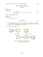
Figure 22.8. Convergence study of SS and clamped square plates under concentrated central load.

energy accuracy.
Figure 22.8 displays log-log error plots in which d is shown as a function of log2 N . The ultimate slope of
the log-log curve characterizes the asymptotic energy convergence rate. The plots indicate an asymptotic
rate of O(1/N 2 ) for all elements, meaning that ultimately a doubling of N gives log10 4 ≈ 0.6 more
digits. The same O(h 2 ) convergence rate was obtained for energy, displacements, centroidal curvatures
and centroidal moments, although only displacements are reported here.
Although the asymptotic convergence rate is the same for all elements in the template, big differences
as regards error coefficients can be observed. These differences are visually dampened by the log scale.
In both problems the difference between the worst element (HCT) and the best ones (HCTS, MDIT1,
AQR1) spans roughly two orders of magnitude. The performance of the new BE and DBE elements
depends significantly on the α parameter, with DBEN12, DBEN13 and DBE12 generally outperforming
the others. The sanitized BCZ elements do well. DKT, FF0 and FF1 come in the middle of the pack.
The results for distributed loads, not reported here, as well 2:1 rectangular plates largely corroborate
these rankings, except for deteriorating performance of the BCZ elements.
§22.8.2. Uniformly Loaded Cantilever
Figure 22.9 reports the convergence study of a narrow cantilever plate subjected to uniform lateral load
q. The aspect ratio is r = 20. Regular N × N meshes are used, with N = 1, 2, 4 and 8. The consistent
transformation of q to node forces has not been investigated. The analysis uses the consistent loads of
FF0, for which the transverse displacement over the triangle is available. This shortcut is not believed
to have a major effect on convergence once the mesh is sufficiently fine.
As expected the beam-exact elements do much better than the others, with an accuracy advantage of 3-4
orders of magnitude for N ≥ 4. (The different superconvergence slopes have not been explained yet in
term of asymptotic expansions, pending a study of consistent load formulations.) The accuracy “spike”
of DBE13 is a fluke caused by computed end deflections crossing over the exact answer before returning
to it.
§22.8.3. Aspect Ratio Test of End Loaded Cantilever

22–22


22–23

§22.8

d (digits of accuracy
in end deflection)

6

5
BTE13

Uniform load q

BENCHMARK STUDIES

DBEN13
DBTE13
DBE13
AQRBE
DBEN00
DBE00=ALR
DBE12
DBEN12

4

t

3

L

L /r
AQR0

2
Plate not drawn to scale for r = 20.
N = 2 mesh shown. End deflection
rapidly approaches qL4 /(8EI),
I = (L/r) t 3 /12, as r grows

DBE23
AQR1
DKT,HCT,
HCTS,MDIT1
AVG,BCIZ0,
BCIZ1,FF0,FF1

DBEsqrt2
1

0

1

Narrow Cantilever Plate, r = 20

Under Uniform Load
N x N Mesh over Full Plate
N
16
2
4
8

Figure 22.9. Convergence study on uniform loaded, narrow cantilever plate.

Aspect ratio tests use a single mesh unit of length L and width b = L/r subjected to simple end load
systems. Only r is varied. Two kinds of tests, depicted in Figures 22.10 and 22.11, were carried out.
The analysis of the shear-end-loaded cantilever mesh unit, reported in Figure 22.10, simply confirms the
asymptotic analysis of the beam morphing process. As expected, the BE and DBE elements designed
to beam-morph exactly perform well, converging to the correct thin-cantilever answer P L 3 /(3E I ) as
r → ∞. All other elements stay at the same deflection percentage beyond r > 8. For example, the
five elements AVG, BCIZ0, BCIZ1, FF0 and FF1 yield 2/3 of the correct answer whereas DKT, MDIT1
yields 3/4 of it.
The end load system must include two fixed-end moments ±α P Lr/12 to deliver the correct answers
predicted by the r → ∞ asymptotic analysis. Should the moments be removed, significant errors occur
if α = 0, and BME mesh units no longer converge to the correct answer as r → ∞. Of course, in the
case of a repeated mesh subdivision the effect of those moments would become progressively smaller.
§22.8.4. Aspect Ratio Test of Twisted Ribbon
Aspect ratio tests were also conducted on a twib subjected to a total applied end torque T using a single
mesh unit fabricated of 4 overlaid triangles to avoid directional anisotropy. The consistent nodal force
system shown in Figure 22.11 was used. Two boundary condition cases: (I) and (II), also defined in
Figure 22.11, were considered.
Case (I) is essentially a constant twist-moment patch test. All elements in the KPT-1-36 template must
pass the test, and indeed all elements gave the correct answer for any r . The total angle of twist must
be φ E = T L/G J , where G = 12 E (because ν = 0) and J = 13 (L/r )t 3 . With the boundary conditions

set as shown, the x rotations at both end nodes must be φ E , the transverse deflections ±φ E (L/2r ) and
the y rotations ±φ E /(2r ). Note, however, that if the applied load system shown in Figure 22.11 is not
adhered to, the patch test is not passed. For example, the end moments cannot be left out unless α = 1.
22–23


22–24

Chapter 22: RECENT ADVANCES IN FINITE ELEMENT TEMPLATES

8

d (digits of accuracy
in end deflection)

z
y

AQRBE

6

B

L /r
A

t
L

P/2
P/2
__
E D _ α PLr
12
C
x
__
αPLr
12

DBE00,DBE13,DBE12
DBEsqrt2
DBE23
BTE13
DBEN13
DBEN12
DBEN00=ALR
DBTE13

4

2
DKT,HCTS,MDIT1

Exact end deflection rapidly approaches PL 3 /(3EI),
I = (L/r)t 3/12 (since ν = 0) as r grows. Reported end
deflection is average of that computed at C and D.
0

AQR1
AQR0
HCT
AVG,BCIZ0,BCIZ1,FF0,FF1

8

16

32

64

r

Figure 22.10. Aspect ratio study of end-loaded cantilever mesh unit.

This consistency result is believed to be new.
Case (II) is analogous to Robinson’s twisted ribbon test [34], which is usually conducted with specific
material and geometric properties. Working with symbolic algebraic computations there is no need to
chose arbitrary numerical values. The end torque T was simply adjusted so that the pure twist solution
gives φ E = r . The graph shown on the right of Figure 22.11 plots φ E as function of r for specific
elements in the range r = 5 to r = 40. Because the sign of the discrepancy is important, this plot does
not use a log-log reduction. It is seen that most elements are too stiff, and that several of them, notably
HCT, BCIZ and FF, exhibit severe aspect ratio locking. For the twib-exact (TE) elements, a symbolic
analysis predicted that exact agreement with the pure twist solution for this boundary condition case can
only be obtained if α = 1/3. The computed response of BTE13 and DBTE13 verifies this prediction.
§22.8.5. The Score so Far
The benchmarks conducted so far, of which those reported in Section 8 constitute a small sample, suggest
that the choice of an optimal “element for all seasons” will not be realized. For the classical rectangular

plate benchmarks HCTS, MDTI1 and AQR1 consistently came at the top. The displacement-assumed
HCT, BCZ and FF elements, which represent 1970-80 technology, did well for unit aspect ratios but
deteriorated for narrower triangles. The new BE and DBE elements showed variable performance. The
performance of DKT was mediocre to average. Skew plate tests, not reported here, were inconclusive.
For problems typified by uniaxial bending of long cantilevers, the BE and DBE elements outperformed
all others as can be expected by construction. The displacement assumed elements did poorly. Distortion
benchmarks, not reported here, indicate that ARI elements with α = 1 outperform elements with α = 1,
or non-ARI elements such as FF1 or HCT.
Based on the test set, MDIT1 and HCTS appear to the running neck and neck as the best all-purpose
KPT elements, closely followed by AQR1. There are arguments for DBE13 as good choice for very
high aspect ratio situations such as the stiffened panels illustrated in Figure 22.7. Unfortunately directly
22–24


22–25

§22.9
z

θyB

y
A

L /r

CONCLUDING REMARKS

θyA = _ θyB

B

Case (I)

40

L
Tz r/L

t

E
Ty r/2

C

_T r/L
z

DBE00
DBE13
AQRBE
BTE13 & DBTE13
DBE12
DBEN13
DBEN00
DBEN12

_T r/2
y

D

30

Tx /2
Tx /2

x

20

same end loads
as in (I)

Pure twist
solution
DBEsqrt2

E

10
BCIZ0

For internal force consistency the total end torque T must be

T = Tx + Ty + Tz,

DKT
AVG

MDIT1
AQR0
HCTS
AQR1
ALR
MDIT13
DBE23

all DOFs fixed

Case (II)

End twist angle φ E
for Case (II)

Tx = α T,

1_α
T
Ty = Tz =
2

HCT

0

Case (I) is a constant-twist patch test. y rotations at A and B
must be allowed under the antisymmetric constraint shown. All
elements must recover the pure twist answer φE = TL/(GJ),
G = E/2, J = (L/r) t 3/12. Case (II) fixes all freedoms at A and B.

5 10

BCIZ1

20

FF0 FF1

30

40 L/r

Figure 22.11. Twisted ribbon test.

joining elements with different αs would violate the IET. Thus a mesh with, say, DBE13 in high aspect
ratio regions and HCTS otherwise would be disallowed. Such combinations could be legalized by
interface transition elements but that would represent a new research topic.
§22.9. CONCLUDING REMARKS
The usual finite element construction process, which involves a priori selection of a variational principle
and shape functions, hinders the exploration of a wide range of admissible finite element models. As
such it is ineffectual for the design of finite elements with desirable physical behavior. The application
described here illustrates the effectiveness of templates to build custom elements. The template approach
attempts to implement the hope long ago expressed by Bergan and Hanssen [24] in the Introduction of
their MAFELAP II paper:
“An important observation is that each element is, in fact, only represented by the numbers in its stiffness
matrix during the analysis of the assembled system. The origin of these stiffness coefficients is unimportant
to this part of the solution process ... The present approach is in a sense the opposite of that normally used
in that the starting point is a generally formulated convergence condition and from there the stiffness matrix
is derived ... The patch test is particularly attractive [as such a condition] for the present investigation in that

it is a direct test on the element stiffness matrix and requires no prior knowledge of interpolation functions,
variational principles, etc.”

This statement sets out what may be called the direct algebraic approach to finite elements: the element
stiffness is derived directly from consistency conditions — provided by the IET — plus stability and
accuracy considerations to determine algebraic redundancies if any. It has in fact many points in common
with energy-based finite differences.
This ambitious goal has proven elusive because the direct algebraic construction of the stiffness matrix
of most multidimensional elements becomes effectively a problem in constrained optimization. In
22–25