The proper generalized decomposition for advanced numerical simulations ch23

23

.

Optimal Membrane
Triangles with
Drlling Freedoms

23–1


23–2

Chapter 23: OPTIMAL MEMBRANE TRIANGLES WITH DRLLING FREEDOMS

TABLE OF CONTENTS
Page

§23.1. INTRODUCTION
§23.2. ELEMENT DERIVATION APPROACHES
§23.2.1. Fixing Up
. . . . . . . . . . . . . .
§23.2.2. Retrofitting
. . . . . . . . . . . . . .
§23.2.3. Direct Fabrication . . . . . . . . . . . .
§23.2.4. A Warning . . . . . . . . . . . . . . .
§23.3. A GALLERY OF TRIANGLES
§23.4. THE ANDES TRIANGLE WITH DRILLING FREEDOMS
§23.4.1. Element Description . . . . . . . . . . .
§23.4.2. Natural Strains
. . . . . . . . . . . . .

§23.4.3. Hierarchical Rotations
. . . . . . . . . .
§23.4.4. The Stiffness Template . . . . . . . . . . .
§23.4.5. The Basic Stiffness
. . . . . . . . . . .
§23.4.6. The Higher Order Stiffness
. . . . . . . . .
§23.4.7. Instances, Signatures, Clones . . . . . . . .
§23.4.8. Energy Orthogonality . . . . . . . . . . .
§23.4.9. Other Templates
. . . . . . . . . . . .
§23.5. FINDING THE BEST
§23.5.1. The Bending Test
. . . . . . . . . . . .
§23.5.2. Optimality for Isotropic Material . . . . . . .
§23.5.3. Optimality for Non-Isotropic Material . . . . . .
§23.5.4. Multiple Element Layers
. . . . . . . . .
§23.5.5. Is the Optimal Element Unique?
. . . . . . .
§23.5.6. Morphing
. . . . . . . . . . . . . .
§23.5.7. Strain and Stress Recovery
. . . . . . . . .
§23.6. A MATHEMATICA IMPLEMENTATION
§23.7. RETROFITTING LST
§23.7.1. Midpoint Migration Migraines . . . . . . . .
§23.7.2. Divide and Conquer . . . . . . . . . . . .
§23.7.3. Stiffness Matrix Assessment
. . . . . . . .

§23.7.4. Deriving a Mass Matrix
. . . . . . . . . .
§23.8. THE ALLMAN 1988 TRIANGLE
§23.8.1. Shape Functions
. . . . . . . . . . . .
§23.8.2. Variants . . . . . . . . . . . . . . . .
§23.9. NUMERICAL EXAMPLES
§23.9.1. Example 1: Cantilever under End Moment . . . .
§23.9.2. Example 2: The Shear-Loaded Short Cantilever
. .
§23.9.3. Example 3: Cook’s Problem
. . . . . . . .
§23.10. DISCUSSION AND CONCLUSIONS
§A23. The Higher Order Strain Field
§23.A.1. The Pure Bending Field
. . . . . . . . . .
§23.A.2. The Torsional Field
. . . . . . . . . . .
§B23. Solving Polynomial Equations for Template Optimality
Acknowledgements
. . . . . . . . . . . . . . . . . . .
References
. . . . . . . . . . . . . . . . . .

. .
.
. .
.

.

. .
.
. .

. .
.
. .
.

. .
.
. .
.
. .
.
. .
.
. .

.
. .
.
. .
.
. .
.
. .
.

. .

.
. .
.
. .
.
. .
.
. .

.
. .
.
. .
.
. .
.

. .
.
. .
.
. .
.
. .

.
. .
.
. .
.

. .
.

. .
.
. .
.

.
. .
.
. .

. .
.
. .
.

. . . . .
. . . .
. . . . .
. . . .
. . . . .

. . . .
. . . . .
. . . .
. . . . .

23–1

23–2
23–2
23–3
23–3
23–3
23–3
23–5
23–6
23–7
23–8
23–9
23–10
23–11
23–13
23–13
23–13
23–13
23–14
23–16
23–16
23–18
23–18
23–18
23–20
23–20
23–23
23–23
23–24
23–28
23–28

23–29
23–29
23–30
23–31
23–31
23–32
23–34
23–37
23–40
23–40
23–40
23–42
23–43
23–44


23–3

A Study of Optimal Membrane
Triangles with Drilling Freedoms
Carlos A. Felippa
Department of Aerospace Engineering Sciences and
Center for Aerospace Structures
University of Colorado
Boulder, Colorado 80309-0429, USA

SUMMARY
This article compares derivation methods for constructing optimal membrane triangles with corner
drilling freedoms. The term “optimal” is used in the sense of exact inplane pure-bending response of
rectangular mesh units of arbitrary aspect ratio. Following a comparative summary of element formulation approaches, the construction of an optimal 3-node triangle using the ANDES formulation is

presented. The construction is based upon techniques developed by 1991 in student term projects, but
taking advantage of the more general framework of templates developed since. The optimal element
that fits the ANDES template is shown to be unique if energy orthogonality constraints are enforced a
priori. Two other formulations are examined and compared with the optimal model. Retrofitting the
conventional LST (Linear Strain Triangle) element by midpoint-migrating by congruential transformations is shown to be unable to produce an optimal element while rank deficiency is inevitable. Use of
the quadratic strain field of the 1988 Allman triangle, or linear filtered versions thereof, is also unable
to reproduce the optimal element. Moreover these elements exhibit serious aspect ratio lock. These
predictions are verified on benchmark examples.

Keywords: finite elements, templates, high performance, drilling freedoms, triangles, membrane, plane
stress, shell, assumed natural deviatoric strains, hierarchical models, signatures, clones.
Accepted for publication in Comp. Meths. Appl. Mech. Engrg., 2003.

23–3


23–1

§23.1 INTRODUCTION

§23.1. INTRODUCTION
One active area of “finitelementology” is the development of high-performance (HP) elements. The
definition of such creatures is subjective. The writer likes to use a result-oriented definition, as stated
in [1]: “simple elements that provide results of engineering accuracy with coarse meshes.”
But what are “simple” elements? Again that term is subjective. The writer’s definition is: elements
with only corner nodes and physical degrees of freedom. Following the high-order element frenzy of
the late 1960s and 1970s, the back trend towards simplicity was noted as early as 1986 by the father of
NASTRAN: “The limitations of higher order elements set out by Zienkiewicz have proved themselves
in application. As a practical matter, the real choice is between lowest order elements (constant strain,
probably with some linear strain terms) and next-lowest-order elements (linear strain, possibly with

some quadratic strain terms), because these are the ones that developers of finite element programs have
found to be commercially viable” [2, p. 89].
The trend has strenghtened since that statement because commercial FEM codes are now used by
comparatively more novices, often as backend of CAD studies. These users have at best only a foggy
notion of what goes on inside the black boxes. Hence the writer’s admonition in an introductory FEM
course: “never, never, never use a higher order or special element unless you are absolutely sure of what
you are doing.” The attraction of HP elements in the real world is understandable: to get reasonable
answers with models that cannot stray too far from physics.
An optimal element is one whose performance cannot be improved for a given node-freedom configuration. The concept is fuzzy, however, unless one specifies precisely what is the optimality measure.
There are often tradeoffs. For example, passing patch tests on any mesh may conflict with insensitivity
to mesh distortion [2, p. 115].
One of the side effects of interest in high performance is the proliferation of elements with drilling
degrees of freedom (DOFs). These are nodal rotations that are not taken as independent DOFs in
conventional elements. Two well known examples are: (i) corner rotations normal to the plane of a
membrane element (or to the membrane component of a shell element); (ii) three corner rotations added
to solid elements. This paper considers only (i).
Why membrane drilling freedoms? Three reasons are given in the Introduction to [3]:
1.

The element performance may be improved without adding midside nodes, keeping model preparation and mesh generation simple.

2.

The extra degree of freedom is “free of charge” in programs that carry six DOFs per node, as is
the case in most commercial codes.

3.

It simplifies the treatment of shell intersections as well as connection of shells to beam elements.

The purpose of this paper is to review critically several approaches for the construction of these elements.
To keep the exposition to a reasonable length, only triangular membrane elements with 3 corner nodes
are studied.

1


Chapter 23: OPTIMAL MEMBRANE TRIANGLES WITH DRLLING FREEDOMS

23–2

FIX-UP APPROACH,
a.k.a. "Shooting"
Improvable
element
Improve element
by medication

RETROFITTING APPROACH
"Parent"
Element

Make descendants

High
Performance
Element
Sometimes
possible

Build from scratch
in stages

DIRECT FABRICATION APPROACH
Piece 1

+

Optimal
Element

Piece 2 + ....

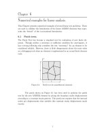
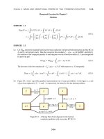
Figure 23.1. Element derivation approaches, not to be confused with methods.

§23.2. ELEMENT DERIVATION APPROACHES
The term approach is taken here to mean a combination of methods and empirical tools to achieve a given
objective. In FEM work, isoparametric, stress-assumed-hybrid and ANS (Assumed Natural Strain)
formulations are methods and not approaches. An approach may zig-zag through several methods.
FEM approaches range from heuristic to highly analytical. The experience of the writer in teaching
advanced FEM courses is that even bright graduate students have trouble connecting different construction methods, much as undergraduates struggle to connect mathematics and laws of nature. To help
students the writer has grouped element derivation approaches into those pictured in Figure 1.
Figure 1 makes an implicit assumption: the performance of an element of given geometry, node and
freedom configuration can be improved. There are obvious examples where this is not possible. For
example, constant-strain elements with translational freedoms only: 2-node bar, 3-node membrane
triangle and 4-node elasticity tetrahedron. Those cases are excluded because it makes no sense to talk
about high performance or optimality under those conditions.
§23.2.1. Fixing Up
Conventional element derivation methods, such as the isoparametric formulation, may produce bad or
mediocre low-order elements. If that is the case two questions may be raised:

(i) Can the element be improved?
(ii) Is the improvement worth the trouble?
If the answer to both is yes, the fix-up approach tries to improve the performance by an array of remedies
that may be collectively called the FEM pharmacy. Cures range from heuristic tricks such as reduced
and selective integration to more scientifically based concoctions.
This approach accounts for most of the current publications in finitelementology. Playing doctor can
be fun. But also frustating, as trying to find a black cat in a dark cellar at midnight. Inject these
2


23–3

§23.3 A GALLERY OF TRIANGLES

incompatible modes: oops! the patch test is violated. Make the Jacobian constant: oops! it locks in
distortion. Reduce the integration order: oops! it lost rank sufficiency. Split the stress-strain equations
and integrate selectively: oops! it is not observer invariant. And so on.
§23.2.2. Retrofitting
Retrofitting is a more sedated activity. One begins with a irreproachable parent element, free of obvious
defects. Typically this is a higher order iso-P element constructed with a complete or bicomplete
polynomial; for example the 6-node quadratic triangle or the 9-node Lagrange quadrilateral. The parent
is fine but too complicated to be an HP element. Complexity is reduced by master-slave constraint
techniques so as to fit the desired node-freedom configuration pattern.
This approach commonly makes use of node and freedom migration techniques. For example, drilling
freedoms may be defined by moving translational midpoint or thirdpoint freedoms to corner rotations by
kinematic constraints. The development of “descendants” of the LST element discussed in Section 7 fits
this approach. Discrete Kirchhoff constraints and degeneration (3D→2D) for plate and shell elements
provide another example. Retrofitting has the advantage of being easy to understand and teach. It
occasionally produces useful elements but rarely high performance ones.
§23.2.3. Direct Fabrication

This approach relies on divide and conquer. To give an analogy: upon short training a FEM novice
knows that a discrete system is decomposed into elements, which interact only through common freedoms. Going deeper, an element can be constructed as the superposition of components or pieces, with
interactions limited through appropriate orthogonality conditions. (Mathematically, components are
multifield subspaces [4].) Components are invisible to the user once the element is implemented.
Fabrication is done in stages. At the start there is nothing: the element is without form, and void. At
each stage the developer injects another component (= subspace). Components may be done through
different methods. The overarching principle is correct performance after each stage. If at any stage the
element has problems (for example: it locks) no retroactive cure is attempted as in the fix-up approach.
Instead the component is trashed and another one picked. One never uses more components than strictly
needed: condensation is forbidden. Components may contain free parameters, which may be used to
improve performance and eventually to try for optimality. One general scheme for direct fabrication is
the template approach [5].
All applications of the direct fabrication method to date have been done in two stages, separating the
element response into basic and higher order. This process is further elaborated in Section 4.3.
§23.2.4. A Warning
The classification of Figure 1 is based on approaches and not methods. A method may appear in
more than one approach. For example, methods based on hybrid functionals may be used to retrofit
or to fabricate, and even (more rarely) to fix up. Methods based on assumed strain or incompatible
displacement fields may be used to do all three. This interweaving of methods and approaches is what
makes so difficult to teach advanced FEM. While it is relatively easy to teach methods, choosing and
pursuing an approach is a synthesis activity that relies on judgement, experience and luck.
§23.3. A GALLERY OF TRIANGLES
This article looks at triangular membrane elements in several flavors organized along family lines. To
keep track of parents and siblings it is convenient to introduce the following notational scheme for the
3


23–4

Chapter 23: OPTIMAL MEMBRANE TRIANGLES WITH DRLLING FREEDOMS

ux3 ,u y3

ux3 ,u y3

u x3 , uy3 ,θz3

3

3

3
ux6 ,uy6
y

2

u x2 ,u y2
ux1 ,u y1

ux1 ,u y1
x

ux8 ,uy8
ux9 ,uy9
1
ux1 ,u y1

8
6 ux6 ,uy6

0
ux0 ,uy0
9
2
ux2 ,uy2
5
4
ux5 ,uy5
ux4 ,uy4

QST-10/20C (Parent)

ux8 ,uy8
ux9 ,uy9
1
ux1 ,u y1

ux3 , uy3
ux,x3, uy,x3
ux,y3, uy,y3

8

ux3 ,u y3
3
7 ux7 ,u y7

1
u x1 , uy1
ux,x1, uy,x1

ux,y1, uy,y1
QST-4/20G

2
ux2 , uy2
1
ux,x2, uy,x2
ux,y2, uy,y2 u x1 , uy1
θ z1 , exx1
e yy1 , exy1

0
ux0 ,u y0

2
u x2 , uy2
θ z2 , exx2
e yy2 , exy2

QST-4/20RS

u x3 , uy3
θ z3 , exx3
e yy3 , exy3 3

6 ux6 ,uy6

9
2
ux2 ,uy2

5
4
ux5 ,uy5
ux4 ,uy4

QST-9/18C

3

3

LST-3/9R
u x3 , uy3
θ z3 , exx3
e yy3 , exy3 3

0
ux0 ,u y0

ux3 , uy3
ux,x3, uy,x3
ux,y3, uy,y3

2
u x2 , uy2 ,θz2

1
u x1 , uy1 ,θz1

LST-6/12C (Parent)

CST-3/6C (Parent)
ux3 ,u y3
3
7 ux7 ,u y7

2
ux2 ,uy2

4
ux4 ,uy4

1

1

u x5 ,u y5

5

6

1
u x1 , uy1
ux,x1, uy,x1
ux,y1, uy,y1
QST-3/18G

2
u x2 , uy2

1
ux,x2, uy,x2
ux,y2, uy,y2 u x1 , uy1
θ z1 , exx1
e yy1 , exy1

2
u x2 , uy2
θ z2 , exx2
eyy2 , exy2

QST-3/18RS

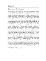
Figure 23.2. Node and freedom configuration of triangular membrane element families.
Only non-hierarchical models with Cartesian node displacements are shown.

4


23–5

§23.4 THE ANDES TRIANGLE WITH DRILLING FREEDOMS

;;; ;;;
;;; ;;;
(a) Parent (LST-6/12C)

(b) Descendant (LST-3/9R)
3

3

z
y

6

5

x

θz

1

1

uy

4

2

2

ux

uy
ux

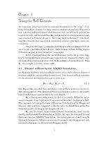
Figure 23.3. Node and freedom configuration of the membrane
triangle LST-3/9R and its parent element LST-6/12C.

configuration of an element:
xST-n/m[variants][-application]

(23.1)

Lead letter x is C, L or Q, which fingers the parent element as indicated below. Integers n and m
give the total number of nodes and freedoms, respectively. Further distinction is made by appending
letters to identify variants. For example QST-10/20C, QST-3/20G and QST-3/20RS identify the QST
parent and two descendants. Here C, G and RS stand for “conventional freedoms”, “gradient freedoms”
and “rotational-plus-strain freedoms,” respectively. The reader may see examples of this identification
scheme arranged in Figure 2.
The three parent elements shown there are generated by complete polynomials. They are:
1.

Constant Strain Triangle or CST. Also called linear triangle and Turner triangle. Developed as
plane stress element by Jon Turner, Ray Clough and Harold Martin in 1952–53 [6]; published 1956
[7].

2.

Linear Strain Triangle or LST. Also called quadratic triangle and Veubeke triangle. Developed by
B. Fraeijs de Veubeke in 1962–63 [8]; published 1965 [9].

3.

Quadratic Strain Triangle or QST. Also called cubic triangle. Developed by the writer in 1965;
published 1966 [10]. Shape functions for QST-10/20RS to QST-3/18G were presented there but

used for plate bending instead of plane stress; e.g., QST-3/18G clones the BCIZ element [11].

Drilling freedoms in triangles were used in static and dynamic shell analysis in Carr’s thesis under
Ray Clough [12,13], using QST-3/20RS as membrane component. The same idea was independently
exploited for rectangular and quadrilateral elements, respectively, in the theses of Abu-Ghazaleh [14]
and Willam [15], both under Alex Scordelis. A variant of the Willam quadrilateral, developed by Bo
Almroth at Lockheed, has survived in the nonlinear shell analysis code STAGS as element 410 [16].
(For access to pertinent old-thesis material through the writer, see References section.)
The focus of this article is on LST-3/9R, shown in the upper right corner of Figure 2 and, in 3D view,
in Figure 3(b). The whole development pertains to the membrane (plane stress) problem. Thus no
additional identifiers are used. Should the model be applied to a different problem, for example plane
strain or axisymmetric analysis, an application identifier would be necessary under scheme (23.1).
§23.4. THE ANDES TRIANGLE WITH DRILLING FREEDOMS
As pictured in in Figure 3(b), the LST-3/9R membrane triangle has 3 corner nodes and 3 DOFs per node:
two inplane translations and a drilling rotation. In the retrofitting approach studied in Section 7 the
parent element is the conventional Linear Strain Triangle, which is technically identified as LST-6/12C.
5


23–6

Chapter 23: OPTIMAL MEMBRANE TRIANGLES WITH DRLLING FREEDOMS

(a)

n6 =n13

(b)

3 (x3 , y3)

3

s6 = s13

t 6 = t13

6

1 (x1, y1 )

6
1

s5 = s32

0

n4 =n 21
x
l21

n 5 = n32

4

t 5 = t32

5

5

y

z

m 6 = m13

4

s4 = s21
2 (x2 , y2) a 3 = a 21

m5 = m 32

t 4= t 21
m4 = m 21

2

Figure 23.4. Triangle geometry.

The direct fabrication approach was used in a three-part 1992 paper [3,17,18] to construct an optimal
version of LST-3/9R. (This work grew out of student term projects in an advanced finite element course.)
Two different techniques were used in that development:
EFF. The Extended Free Formulation, which is a variant of the Free Formulation (FF) of Bergan [19–27].
ANDES. The Assumed Natural DEviatoric Strain formulation, which combines the FF of Bergan and
a variant of the Assumed Natural Strain (ANS) method due to Park and Stanley [28,29]. ANDES has
also been used to develop plate bending and shell elements [30,31].
For the LST-3/9R, these techniques led to stiffness matrices with free parameters: 3 and 7 in the case of

EFF and ANDES, respectively. Free parameters were optimized so that rectangular mesh units are exact
in pure bending for arbitrary aspect ratios, a technique further discussed in Section 5. Surprisingly the
same optimal element was found. In the nomenclature of templates summarized in Section 4.7 the two
elements are said to be clones. This coalescence nurtured the feeling that the optimal form is unique.
More recent studies reported in Section 5.5 verify uniqueness if certain orthogonality constraints are
placed on the higher order response.
§23.4.1. Element Description
The membrane (plane stress) triangle shown in Figure 4 has straight sides joining the corners defined
by the coordinates {xi , yi }, i = 1, 2, 3. Coordinate differences are abbreviated xi j = xi − x j and
yi j = yi − y j . The signed area A is given by
2A = (x2 y3 − x3 y2 ) + (x3 y1 − x1 y3 ) + (x1 y2 − x2 y1 ) = y21 x13 − x21 y13

(and 2 others).

(23.2)

In addition to the corner nodes 1, 2 and 3 we shall also use midpoints 4, 5 and 6 for derivations although
these nodes do not appear in the final equations of the LST-3/9R. Midpoints 4, 5, 6 are located opposite
corners 3, 1 and 2, respectively. The centroid is denoted by 0. As shown in Figure 4, two intrinsic
coordinate systems are used over each side:
n 21 , s21 ,

n 32 , s32 ,

n 13 , s13 ,

(23.3)

m 21 , t21 ,

m 32 , t32 ,

m 13 , t13 .

(23.4)

6


23–7

§23.4 THE ANDES TRIANGLE WITH DRILLING FREEDOMS

Here n and s are oriented along the external normal-to-side and side directions, respectively, whereas
m and t are oriented along the triangle median and normal-to-median directions, respectively. The
coordinate sets (23.3)–(23.4) align only for equilateral triangles. The origin of these systems is left
“floating” and may be adjusted as appropriate. If the origin is placed at the midpoints, subscripts 4, 5
and 6 may be used instead of 21, 32 and 13, respectively, as illustrated in Figure 4.
Other intrinsic dimensions of use in element derivations are
ij

=

ji

=

xi2j + yi2j ,

ai j = ak = 2A/

ij,

mk =

3
2

2
2
xk0
+ yk0
,

bk = 2A/m k ,

(23.5)

Here j and k denote the positive cyclic permutations of i; for example i = 2, j = 3, k = 1. The i j ’s
are the lengths of the sides, ak = ai j are triangle heights, m k are the lengths of the medians, and bk are
side lengths projected on normal-to-median directions.
The well known triangle coordinates are denoted by ζ1 , ζ2 and ζ3 , which satisfy ζ1 + ζ2 + ζ3 = 1.
The degrees of freedom of LST-3/9R are collected in the node displacement vector
u R = [ u x1 u y1 θ1 u x2 u y2 θ2 u x3 u y3 θ3 ]T .

(23.6)

Here u xi and u yi denote the nodal values of the translational displacements u x and u y along x and y,
respectively, and θ ≡ θz are the “drilling rotations” about z (positive counterclockwise when looking
down on the element midplane along −z). In continuum mechanics these rotations are defined by

θ = θz =

1
2

∂u y
∂u x
−
∂x
∂y

.

(23.7)

The triangle will be assumed to have constant thickness h and uniform plane stress constitutive properties.
These are defined by the 3 × 3 elasticity and compliance matrices arranged in the usual manner:

E=

E 11
E 12
E 13

E 12
E 22
E 23

E 13
E 23

E 33

,

C = E−1 =

C11
C12
C13

C12
C22
C23

C13
C23
C33

.

(23.8)

For later use six invariants of the elasticity tensor are listed here:
JE1 = E 11 + 2E 12 + E 22 ,

JE2 = −E 12 + E 33 ,

JE3 = (E 11 − E 22 )2 + 4(E 13 + E 23 )2 ,

JE4 = (E 11 − 2E 12 + E 22 − 4E 33 )2 + 16(E 13 − E 23 )2 ,

2
2
2
JE5 = det(E) = E 11 E 22 E 33 + 2E 12 E 13 E 23 − E 11 E 23
− E 22 E 13
− E 33 E 12
,
3
2
2
2
2
3
+ E 12 E 13 E 22 − E 13 E 22
+ E 11
E 23 + 2E 13
E 23 + E 12 E 22 E 23 − 2E 13 E 23
− 2E 23
+
JE6 = 2E 13
2E 22 (E 13 + E 23 )E 33 − E 11 (E 12 E 13 − E 13 E 22 + E 12 E 23 + E 22 E 23 + 2(E 13 + E 23 )E 33 ).
(23.9)
Of these JE1 , JE2 and JE5 are well known, while the others were found by Mathematica.

7


23–8

Chapter 23: OPTIMAL MEMBRANE TRIANGLES WITH DRLLING FREEDOMS

1

(s)

3

ε21

ε13

(m)

(n)

3

εm2

1

εm3

ε32

1

εm1

2

3

1

2

2

Along side directions

(t)

3

Along medians

Along normal to sides

2
Along normal to medians

Figure 23.5. Four choices for natural strains. Labels (s) through (t) correlate with the notation
(23.3)-(23.4). Although the “natural straingage rosettes” are pictured at the centroid
for viewing convenience, they may be placed at any point on the triangle.

§23.4.2. Natural Strains
In the derivation of the higher order stiffness by ANDES [17] natural strains play a key role. These
are extensional (direct) strains along three directions intrinsically related to the triangle geometry. Four
possible choices are depicted in Figure 5. Choice (s): strains along the 3 side directions, was the one

used in [17] because it matches the direction of neutral axes of the assumed inplane bending modes as
discussed in Section 4.6.
The (s) natural strains are collected in the 3-vector
=[

21

32

13

]T .

(23.10)

Vector at point i is denoted by i . The natural strain jk at point i will be written jk|i , the bar being
used for reading convenience. The natural strains are related to Cartesian strains {ex x , e yy , 2ex y } by the
“straingage rosette” transformation


=

12
23
31

in which
ex x
e yy
2ex y

2
ji

2
x21
/
2
=  x32 /
2
x13
/

2
21
2
32
2
13

2
y21
/
2
y32 /
2
y13
/

2

21
2
32
2
13

x21 y21 /
x32 y32 /
x13 y13 /

2
21
2
32
2
13




ex x
e yy
2ex y

= T−1
e e,

(23.11)

= x 2ji + y 2ji . The inverse relation is



y23 y13 221
1 
=
x23 x13 221
4A2
(y23 x31 + x32 y13 )

2
21

y31 y21 232
x31 x21 232
(y31 x12 + x13 y21 )

2
32

y12 y32 213
x12 x32 213
(y12 x23 + x21 y32 )



2
13

12
23

31

,

(23.12)
or, in compact matrix notation, e = Te . Note that Te is constant over the triangle. The natural
stress-strain matrix Enat is defined by
(23.13)
Enat = TeT ETe ,
which is also constant over the triangle.
8


23–9

§23.4 THE ANDES TRIANGLE WITH DRILLING FREEDOMS
3

3
Total motion

1
1
2

2

3

3

3

Hierarchical
motion

CST motion
1

+

1

~

θ1

~

θ3

1
~

θ2

2

2

2

Figure 23.6. Decomposition of inplane motion into CST (linear displacement) + hierarchical.
The same idea (in 2D or 3D) is also important in corotational formulations.

§23.4.3. Hierarchical Rotations
Hierarchical drilling freedoms are useful for compactly expressing the higher order behavior of the
element. Their geometric interpretation is shown in Figure 6. To extract the hierarchical corner
rotations θ˜i from the total corner rotations θi , subtract the mean or CST rotation θ0 :
θ˜i = θi − θ0 ,

(23.14)

where i = 1, 2, 3 is the corner index and

θ0 =

1
x23 u x1 + x31 u x2 + x12 u x3 + y23 u y1 + y31 u y2 + y12 u y3 .
4A

(23.15)

Applying (23.14)-(23.15) to the three corners we assemble the transformation

u x1
 u y1 


 θ1 



0  u x2 


0  u y2  = T˜ θu u R .


4A  θ2 


 u x3 


u y3
θ3


˜ 
θ1
˜θ =  θ˜2  = 1
4A
θ˜3

x32
x32
x32

y32
y32

y32

4A
0
0

x13
x13
x13

y13
y13
y13

0
4A
0

x21
x21
x21

y21
y21
y21

(23.16)

For some developments it is useful to complete this transformation with the identity matrix for the
9

23–10

Chapter 23: OPTIMAL MEMBRANE TRIANGLES WITH DRLLING FREEDOMS

translational freedoms:
u





1
0
 u y1  
 

x32

 θ˜1   4A


 u x2  
0
 

 0



u
u˜ R =  y2  = 
x32
 ˜  
 θ2  
4A



0
 u x3  
u  

0
y3
x32
θ˜3
4A
x1

0
1
y32
4A
0
0
y32
4A
0
0

y32
4A

0
0
1
0
0
0
0
0
0

0
0
x13
4A
1
0
x13
4A
0
0
x13
4A

0
0
y13
4A

0
1
y13
4A
0
0
y13
4A

0
0
0
0
0
1
0
0
0

0
0
x21
4A
0
0
x21
4A
1
0
x21

4A

0
0
y21
4A
0
0
y21
4A
0
1
y21
4A



0 
u x1
0
  u y1 


0
  θ1 


0
  u x2 



0   u y2 
 = T˜ R u R .


0   θ2 


u 
0
  x3 
0  u y3
θ3
1

(23.17)

−1
−1
The inverse transformation T˜ R that connects u R = T˜ R u˜ R is obtained by simply transposing the
subscripts in the coordinate differences; x32 → −x32 = x23 , etc. The foregoing transformation matrices
are constant over the element.

§23.4.4. The Stiffness Template
The fundamental element stiffness decomposition of the two-stage direct fabrication method is
K = Kb + K h

(23.18)

Here Kb is the basic stiffness, which takes care of consistency, and Kh is the higher order stiffness,

which takes care of stability (rank sufficiency) and accuracy. This decomposition was found by Bergan
and Nyg˚ard [20] as part of the Free Formulation (FF), but actually holds for any element that passes the
Individual Element Test (IET) of Bergan and Hanssen [32]. (The IET is a strong form of the patch test
that demands pairwise cancellation of tractions between adjacent elements in constant stress states.)
Similar elements were constructed by Belytschko and coworkers [33] using an hourglass stabilization
approach. See also Hughes [34, §4.8].
Orthogonality conditions satisfied by Kh are discussed in [4,19,21–27,35–38].
The EFF and ANDES triangles derived in [3] and [17] initially carry along a set of free numerical
parameters, most of which affect the higher order stiffness:
KEFF’91 (αb , αh , γ ) = Kb (αb ) + (1 − γ )Kuh (αh ),

(23.19)

KANDES’91 (αb , β, ρ1 , . . . ρ5 ) = Kb (αb ) + βKuh (ρ1 , . . . ρ5 ),

(23.20)

where Kuh is the unscaled higher order stiffness. Both Kb and Kh must have rank 3. Algebraic forms
such as (23.19)-(23.20) possessing free parameters are called element stiffness templates or simply
templates.
The basic stiffness Kb (αb ) is identical for both (23.19) and (23.20). In fact, patch test and template
theory [5,35–38] says that Kb (αb ) must be shared by all elements that pass the IET although αb may vary
for different models. However αb must be the same for all LST-3/9R elements connected in an assembly,
for otherwise the patch test would be violated. This is called a mixability condition. Parameters other
than αb may, in principle, vary from element to element without affecting convergence.
10


23–11

§23.4 THE ANDES TRIANGLE WITH DRILLING FREEDOMS

§23.4.5. The Basic Stiffness
An explicit form of the basic stiffness for the LST-3/9R configuration was obtained in 1984 and published
the following year [21]. It can be expressed as
Kb = V −1 L E LT .

(23.21)

where V = Ah is the element volume, and L is a 3 × 9 matrix that contains a free parameter αb :


y23
0

1
 6 αb y23 (y13 − y21 )

y31


L = 12 h 
0
1
 6 αb y31 (y21 − y32 )

y12


0

1
α
y
(y
− y13 )
6 b 12 32

0
x32
1
α x (x − x12 )
6 b 32 31
0
x13
1
α x (x − x23 )
6 b 13 12
0
x21
1
α
x
(x
− x31 )
6 b 21 23


x32
y23



1
α (x y − x12 y21 ) 
3 b 31 13

x13


y31
.

1
α (x y − x23 y32 ) 
3 b 12 21

x21


y12
1
α (x y − x31 y13 )
3 b 23 32

(23.22)

In the FF this is called a force-lumping matrix, hence the symbol L. Under certain conditions L can be
related to the mean strain-displacement matrix B0 or B¯ used in one-point reduced integration schemes:
B0 = LT /V , for specific choices of αb . This matrix also appears in the so-called “B-bar” formulation
[34]. If αb = 0 the basic stiffness reduces to the total stiffness matrix of the CST-3/6C, in which case
the rows and columns associated with the drilling rotations vanish.

One interesting result is that

LT = LT T˜ R ,

(also B0 = B0 T˜ R ),

(23.23)

for any αb , which shows that the transformation (23.17) projects out the higher order behavior.
The deep significance of this development is: the basic stiffness of any element with this node-freedom
configuration that passes the IET must have the form (23.21)–(23.22). Most derivation methods produce
the total stiffness K directly, with Kb concealed behind the scenes. This is one of the reasons accounting
for the capricious nature of the fix-up approach. In the direct fabrication approach the decomposition
(23.18) is explicitly used in the two-stage construction of the element: first Kb and then Kh .
§23.4.6. The Higher Order Stiffness
We describe here essentially the ANDES form of Kh developed in [17], with some generalizations in
the set of free parameters discussed at the end of this subsection. The higher order stiffness matrix is
T
Kh = c f ac T˜ θu Kθ T˜ θu .

(23.24)

where Kθ is the 3 × 3 higher order stiffness in terms of the hierarchical rotations θ˜ of (23.14), Tθu
˜ is
the matrix (23.16), and c f ac is a scaling factor to be determined later. To construct Kθ by ANDES one
picks deviatoric natural strain patterns, in which “deviatoric” means change from the constant strain
states.
Since the main objective is to have good inplane bending behavior, it is logical to begin by assuming
patterns associated with three bending-like modes. A key question is, along which directions? For
11

23–12

Chapter 23: OPTIMAL MEMBRANE TRIANGLES WITH DRLLING FREEDOMS

Bending modes
3

3
1

1

1

2

∼ ∼

∼ ∼

∼
−θ1= θ2 =1, θ3 =0

Torsion mode
3

3

2

1

∼ ∼

∼
−θ2= θ3 =1, θ1 =0

∼
−θ3= θ1 =1, θ2 =0

2

∼ ∼ ∼

θ1= θ2 =θ 3 =1

2

Figure 7. Patterns chosen to build the higher order stiffness of the ANDES template (31):
three bending-along-sides modes plus a torsion mode. Although pictured as
displacement motions for visualization convenience, the bending modes were
initially assumed in natural strains as described in Appendix A. The “neutral axes”
of the bending modes are parallel to the sides and pass through the centroid.

a triangle, four choices — already depicted in Figure 5 as regards the definition of natural strains —
satisfy observer invariance:
Along the side directions s4 , s5 , s6
Along the normal directions n 4 , n 5 , n 6

(23.24)

Along the median directions m 4 , m 5 , m 6

(23.26)

Along the normal-to-the-median directions t4 , t5 , t6

(23.27)

(23.25)

Choice (23.24) was adopted in [17]. The three bending strain patterns are sketched on the left of Figure 7
as displacement modes for visualization convenience. (The bending shapes pictured there were obtained
by integrating the assumed strain fields and adjusting for rigid body motions.) It turns out that the three
patterns are not linearly independent: their sum vanishes for any triangle geometry. Thus use of only
those modes would produce a rank deficient Kh .
To attain the correct rank of 3 the “torsion” pattern depicted on the right of Figure 7 is adjoined. This
can be visualized as produced by applying identical hierarchical rotations θ˜1 = θ˜2 = θ˜3 . A cubic
displacement pattern was constructed from the QST-4/20G interpolation. The associated quadratic
strain pattern was transformed to natural strains and filtered to a linear variation by midpoint collocation.
Those derivations are presented in Appendix A for readers interested in the technical details.
To express Kθ compactly, introduce the following matrices, which depend on nine free dimensionless
parameters, β1 through β9 :
 β
 β
 β
β
β 

β
β 
β
β 
1
2
21

2A
Q1 =
3


 β
 4
 2
 32
 β
7
2
13

2
2
21

β5

2
32

β8

2
13

3
2
21

9
2
21



2A 
β6 

 β3
 2
2  , Q2 =
3  32
32 

 β
β9
6
2
13

2
13

12

7
2
21

β1

2
32

β4

2
13

8
2
21

5
2
21




2A 
β2 

 β8
 2
2  , Q3 =
3  32
32 

 β
β5
3
2
13

2
13

6
2
21

β9

2
32

β1

2

13

4
2
21


β7 

2 .
32 
β2 
2
13

(23.28)


23–13

§23.4 THE ANDES TRIANGLE WITH DRILLING FREEDOMS

The scaling by 2A/3 is for convenience in correlating with prior developments. Matrix Qi relates the
˜ At a point of triangular coordinates
natural strains i at corner i to the deviatoric corner curvatures θ.
˜ where Q = Q1 ζ1 + Q2 ζ2 + Q3 ζ3 . Evaluate this at the midpoints:
{ζ1 , ζ2 , ζ3 }, = Q θ,
Q4 = 12 (Q1 + Q2 ),

Q5 = 12 (Q2 + Q3 ),

Q6 = 12 (Q3 + Q1 )

(23.29)

Then
Kθ = h Q4T Enat Q4 + Q5T Enat Q5 + Q6T Enat Q6 ,

(23.30)

and Kh = 34 β0 TθTu Kθ Tθ u , where β0 is an overall scaling coefficient. (This coefficient could be absorbed
into the βi but it is left separate to simplify the incorporation of material behavior into the optimal
element.) So finally K R assumes a template form with 11 free parameters: αb , β0 , β1 , . . . β9 :
T
K R (αb , β0 , β1 , . . . β9 ) = V −1 LELT + 34 β T˜ θu Kθ T˜ θu .

(23.31)

The factor 34 in Kh comes from “historical grandfathering”: as shown in Section 5 the optimal β0 for
isotropic material with ν = 0 becomes 12 , same as in the 1984 FF element [21]. The template (23.31)
will be called the “LST-3/9R ANDES Template” to distinguish it from others alluded to in Section 4.9.
It is easily checked that if the 3 × 3 matrix with {β1 , β2 , β3 }, {β4 , β5 , β6 } and {β7 , β8 , β9 } as rows is
nonsingular, then Q1 , Q2 and Q3 have full rank for A = 0 and nonzero side lengths. With the usual
restrictions on the elasticity matrix E, Kθ has full rank of 3 and K R is rank sufficient.
As remarked previously, the parameter set in (23.28) is more general than that used in [17]. That
development carried only five free parameters in the Qi matrices: ρ1 through ρ5 , cf. (23.20), which
enforced a priori the triangular symmetry conditions
β7 = −β1 ,

β8 = −β3 ,

β9 = −β2 .

(23.32)

These constraints may be derived, for example, by taking an equilateral triangle in which 21 = 32 = 13
and looking at symmetries about the medians as the θ˜i are applied to each corner in turn. Furthermore
the torsional mode was not separately parametrized. The present parameter set is able to encompass
elements, such as the retrofitted LST, where that mode is missing.
§23.4.7. Instances, Signatures, Clones
An element generated by specifying numerical values to the parameters {αb , β0 , β1 , . . . β9 } is a template
instance. The set of parameter values is the template signature. Two elements with the same signature,
possibly derived through different methods, are called clones.
Table 1 lists triangular elements compared later in this paper. Table 2 defines their signatures if they
happen to be instances of the ANDES template (23.31).
By construction all template instances verify exactly the IET for rigid body modes and uniform
strain/stress states. Here we see the key advantage of the direct fabrication approach: any template instance that keeps the correct rank is guaranteed to be consistent and stable. Since surprises are mitigated
the task of optimizing the element, covered in Section 5, is straightforward.
13


23–14

Chapter 23: OPTIMAL MEMBRANE TRIANGLES WITH DRLLING FREEDOMS

Table 1. Identifier of Triangle Element Instances
Name

Description

See

ALL-3I

Allman 88 element integrated by 3-point interior rule.

Section 8

ALL-3M

Allman 88 element integrated by 3-midpoint rule.

Section 8

ALL-EX

Allman 88 element, exactly integrated

Section 8

ALL-LS

Allman 88 element, least-square strain fit.

Section 8

CST

Constant strain triangle CST-3/6C.

Ref. [7]

FF84

1984 Free Formulation element of Bergan and Felippa.

Ref. [21]

LST-Ret

Retrofitted LST with αb = 4/3.

Section 7

OPT

Optimal ANDES Template.

Sections 5.2 and 5.3

Table 2. Signatures of Some LST-3/9R Instances Befitting the ANDES Template (31)
Name

αb

β0

β1

β2

β3

β4

β5

β6

β7

β8

β9

ALL-3I

1

4/9

1/12

5/12

1/2

0

1/3

−1/3

−1/12

−1/2

−5/12

ALL-3M

1

4/9

1/4

5/4

3/2

0

1

−1

−1/4

−3/2

−5/4

ALL-EX

not an instance of ANDES template
−3/20 −9/10

−3/4

ALL-LS

1

4/9

3/20

3/4

9/10

0

3/5

−3/5

CST

0

any

0

0

0

0

0

0

0

0

0

FF84

not an instance of ANDES template

LST-Ret

4/3

1/2

2/3

−2/3

0

0

−4/3

4/3

−2/3

0

2/3

OPT

3/2

see §5.2

1

2

1

0

1

−1

−1

−1

−2

§23.4.8. Energy Orthogonality
For future use the following definition is noted. An element with linearly varying higher order strains
is called energy orthogonal in the sense of Bergan [19] if Q = Q1 ζ1 + Q2 ζ2 + Q3 ζ3 vanishes at the
centroid ζ1 = ζ2 = ζ3 = 1/3. This gives the algebraic condition
Q1 + Q2 + Q3 = 0.

(23.33)

For the matrices (23.28), condition (23.33) translates to β1 +β5 +β9 = β2 +β6 +β7 = β3 +β4 +β8 = 0.
These conditions are not enforced a priori. The optimal element derived in Section 5, however, is found
to satisfy energy orthogonality.
For more general strain variations energy orthogonality conditions are discussed in [19,21–27,35–38].
§23.4.9. Other Templates
Three more templates for Kh may be generated by choosing bending patterns according to the prescriptions (23.24), (23.25) and (23.26) for the bending modes. This has not been done to date and remains
14

23–15

Mx

Mx

y

z

;;
;;

§23.5 FINDING THE BEST

y

z

b

Cross
section

x

h

y

3

b = a/γ

b

x

1

a

a

2

Figure 8. Constant-moment inplane bending test along the x direction.

an open research problem. The closest attempt in this direction was the development of the 1984 FF
element described in [21,22] by assuming bending modes along the 3 median directions. Because the
FF was used, the modes were initially constructed in displacement form. An advantage of this choice
is that the three modes are linearly independent and there is no need to adjoin the torsional mode. But
perfect optimality in the sense discussed below was not attainable. As there are indications that the
optimal element derivable from (23.31) is unique, as discussed in Section 5.5, there seems to be no
compelling incentive for exploring other templates.
§23.5. FINDING THE BEST
A template such as (23.31) generates an infinity of element instances by assigning numeric values to
the free parameters. The obvious question is: among all those instances, is there a best one? Because
all template instances pass the IET for basic modes (rigid body motions and constant strain states) any
optimality criterion must necessarily rely on higher order patch tests. The obvious tests involve the

response of regular mesh units to inplane bending along the side directions. This leads to element
bending tests expressed as energy ratios. These have been used since 1984 to tune up the higher order
stiffness of triangular elements [21,24].
§23.5.1. The Bending Test
The x-bending test is defined in Figure 8. A Bernoulli-Euler plane beam of thin rectangular crosssection with span L, height b and thickness h (normal to the plane of the figure) is bent under applied
end moments Mx . The beam is fabricated of isotropic material with elastic modulus E and Poisson’s
ratio ν. Except for possible end effects the exact solution of the beam problem (from both the theoryof-elasticity and beam-theory standpoints) is a constant bending moment M(x) = Mx along the span.
1
The stress field is σx x = Mx y/Izz , σ yy = σx y = 0, where Izz = 12
hb3 . Computing the strain field
e = E−1 σ and integrating it one finds the associated displacement field
u x = −κ x y,

u y = 12 κ(x 2 + νy 2 ),

(23.34)

where κ is the deformed beam curvature Mx /E Izz . The internal energy taken up by a Bernoulli-Euler
beam segment of length a is Uxbeam = Mx κa = 6a E Mx2 /(b3 h).
15


23–16

Chapter 23: OPTIMAL MEMBRANE TRIANGLES WITH DRLLING FREEDOMS

To test the ANDES template, the beam is modeled with one layer of identical rectangular mesh units
dimensioned a × b and made up of two LST-3/9R triangles, as illustrated in Figure 9. The aspect ratio
a/b is called γ . All rectangles will undergo the same deformations and stresses. We can therefore
consider a typical mesh unit. Both triangles will absorb the same energy so it is sufficient to take one

triangle and multiply by two. For simplicity begin by taking ν = 0. Evaluating (23.34) at nodes 1-2-3
of the triangle shown at the bottom right of Figure 8 we get the node displacement vector
utrig
x =

3Mx Eγ 2
[ −a
a2h

1
γa
2

−2γ

a

1
γa
2

2γ

a

1
γa
2

(23.35)

−2γ ]T

trig

=
The strain energy absorbed by the triangle under these applied node displacements is Ux
trig
trig
quad
1 trig T
(u
)
Ku
.
That
absorbed
by
the
two-triangle
mesh
unit
is
U
=
2U
.
The
bending
enx

x
x
x
2
ergy ratio computed by Mathematica can be expressed as
quad

Ux
r = beam = c0 + c2 γ 2 + c4 γ 4 ,
Ux

(23.36)

where c0 , c2 and c4 are only functions of the free parameters. For the ensuing derivation we use
the parameters of (23.31), but under the symmetry constraints (23.32) that effectively reduce the 11
parameters to 8: αb , β0 , β1 , . . . β6 . Introduce the 6-vector β = [ β1 β2 β3 β4 β5 β6 ]. Then a
compact form of the coefficients is
c0 =

1
β0
(αb − 6)αb + (βT C0 β),
3
64

c2 =

2
β0
(αb − 3)αb + (βT C2 β),

3
64

c4 =

β0 T
(β C4 β), (23.37)
64

in which C are the symmetric matrices
 13 −11 −1 2 2 −6 
 26 −20 −4 −10 12 −6 
 1 1 −3
 −11 13 −1 −2 −2 6 
 −20 22 −2 8 −14 8 
 1 1 −3
 −1 −1 1 0 0 0 
 −4 −2 6 0 2 0 

 , C2 = 
 , C4 =  −3 −3 9
C0 = 
 2 −2 0 1 1 −3 
 −10 8 0 5 −5 1 
 0 0 0






2 −2
−6
6

0 1 1 −3
0 −3 −3 9

12 −14
−6
8

2 −5
9 −5
0
1 −5 5

0
0

0
0



0 0 0
0 0 0
0 0 0

9 −3 −3 


0 −3 1 1
0 −3 1 1
(23.38)

The energy ratio (23.36) happens to be the ratio of the exact (beam) displacement solution to that of
the 2D solution. Hence r = 1 means that we get the exact answer, that is, the LST-3/9R element is
x-bending exact. If r > 1 or r < 1 the triangle is overstiff or overflexible in x bending, respectively.
In particular, if r >> 1 as a/b = γ grows the element is said to experience aspect ratio locking along
the x direction.
The treatment of energy balance in y bending for rectangular mesh units stacked in the y direction only
entails replacing γ by 1/γ . Therefore if the element is x-bending optimal in the sense discussed below
it is also y-bending optimal and the analysis need not be repeated.
§23.5.2. Optimality for Isotropic Material
If r = 1 for any aspect ratio γ the element is called bending optimal. From (23.36) optimality requires
c0 = 1,

c2 = 0,

c4 = 0,

for all γ = a/b and real parameter values.
16

(23.39)


23–17

§23.5 FINDING THE BEST
Table 3 Bending Energy Ratios r for Triangular Elements of Table 1

γ =0 γ =1
ν = 14 ν = 14

γ =4
ν = 14

584 + (79 − 91ν)γ 2 + 6γ 4
432(1 − ν 2 )

1.442 1.595

7.457 1007.901

ALL-3M

24 + (5 − 9ν)γ 2 + 2γ 4
16(1 − ν 2 )

1.600 1.916 38.667 8786.667

ALL-EX

84 + (15 − 19ν)γ 2 + 2γ 4
60(1 − ν 2 )

1.493 1.711 13.511 2378.311

ALL-LS

1672 + (263 − 371ν)γ 2 + 54γ 4

1200(1 − ν 2 )

1.486 1.686 16.196 3185.956

CST

6 + 3(1 − ν)γ 2
2(1 − ν 2 )

3.200 4.400 22.400

FF84

13 + 54γ 2 + 119γ 4 + 70γ 6 + 13γ 8
3+
13
+
4 96(1 − ν)
96(1 + 3γ 2 + γ 4 )2 (1 + ν)

1.039 1.020

1.035

1.039

LST-Ret

34 + 5(1 − ν)γ 2
27(1 − ν 2 )

1.343 1.491

3.714

39.269

OPT

1

1.000 1.000

1.000

1.000

Triangle

Bending ratio r for isotropic material

ALL-3I

γ = 16
ν = 14

310.400

The last proviso means that complex solutions for template parameters are not admissible. The solution
method is explained in Appendix B. It gives the optimal parameter set

αb = 32 , β0 = 12 , β1 = β3 = β5 = 1, β2 = 2, β4 = 0, β6 = β7 = β8 = −1, β9 = −2,

(23.40)

and the Qi matrices found in [17] are recovered. It is easily verified that r = rb + rh = 3/4 + 1/4,
where rb and rh come from energy taken by the basic and higher-order stiffnesses, respectively. That
is, for the optimal element the basic energy accounts for 75% of the exact beam energy.
The symbolic analysis for an arbitrary ν is similar and shows that only β0 needs to be changed:
αb = 32 , β0 = 12 (1 − 4ν 2 ), β1 = β3 = β5 = 1, β2 = 2, β4 = 0, β6 = β7 = β8 = −1, β9 = −2.
(23.41)
1
1
2
In this case rh = 4 (1 − 4ν ) so for ν = 2 the basic stiffness takes up all the bending energy. Since for
ν = 12 the optimal β0 is 0, the higher order stiffness would vanish and the element is rank deficient. To
maintain stability one sets a tiny minimum β0 , for example β0 = max( 12 (1 − 4ν 2 ), 0.01) is used in our
shell codes. The case of a non-isotropic material is treated in the next subsection.
Table 3 gives bending ratios for the elements listed in Table 1, along with numerical values for ν = 1/4
and γ = 1, 2, 4, 16. Those quoted for elements other than OPT are derived in Sections 7 and 8.
§23.5.3. Optimality for Non-Isotropic Material
If the elasticity matrix takes up the general form (23.8) the analysis of bending optimality becomes more
elaborate, but follows essentially the same steps. Only the final results are stated here. For optimal
17


Chapter 23: OPTIMAL MEMBRANE TRIANGLES WITH DRLLING FREEDOMS

23–18

bending behavior along a direction xϕ that forms an angle ϕ (positive ccw) from x, the optimal parameter

set is still given by (23.41) except for the overall scaling parameter β0 :
2
3
− , ϒ = E 11ϕ C11ϕ ,
ϒ
2
4
= E 11 cϕ + 4E 13 cϕ3 sϕ + (2E 12 + 4E 33 )cϕ2 sϕ2 + 4E 23 cϕ sϕ3 + E 22 sϕ4 ,

β0ϕ =
E 11ϕ

(23.42)

C11ϕ = C11 cϕ4 + 2C13 cϕ3 sϕ + (2C12 + C33 )cϕ2 sϕ2 + 2C23 cϕ sϕ3 + C22 sϕ4 ,
with sϕ = sin ϕ and cϕ = cos ϕ. Here E 11ϕ and C11ϕ are the elasticity and compliance along xϕ ,
respectively, when (23.8) are rotated by ϕ. For isotropic material of Poisson’s ratio ν, ϒ = 1/(1 − ν 2 )
and the rule (23.41) is recovered for any ϕ. Two difficulties, however, arise in the general case:
1.

The optimal β0 depends on orientation of bending actions with respect the element axis. That
information is not likely to be known a priori.

2.

There is no guarantee that ϒ < 4/3, so β0ϕ may turn out to be negative.

The first obstacle is overcome by adopting an invariant measure that involves the average of E 11ϕ C11ϕ
over a 2π sweep:
ϒ¯ =

1
2π

2π

E 11ϕ C11ϕ dϕ =

0

W
,
128 det(E)

β¯0 =

2
3
− .
2
ϒ¯

(23.43)

Mathematica gives W as the complicated expression listed in Figure 12. In terms of the elasticity
3
2
2
3
+ 48JE1

JE2 + JE1 (80JE2
− 10JE3 + JE4 ) + 8(16JE2
−
tensor invariants listed in (23.9), 8W = 9JE1
¯
JE2 (JE3 + JE4 ) + 72JE5 ) so the invariance of β0 is confirmed. The second difficulty is handled by
checking whether β¯0 is less that a positive treshold, say, 0.01 and if so setting β¯0 = 0.01.
What is the effect of setting a β0 that is not exactly optimal? Choosing αb , β1 , . . . β9 as listed in (23.40)
or (23.41) guarantees that c2 = c4 = 0 for any E. Consequently the element cannot lock as the aspect
ratio γ increases. On the other hand c0 will generally differ from one so suboptimal performance can
be expected if the material is not isotropic.
§23.5.4. Multiple Element Layers
Results of the energy bending test can be readily extended to predict the behavior of 2n (n = 1, 2, . . .)
identical layers of elements symmetrically placed through the beam height. If γ stays constant, the
energy ratio becomes
22n − 1 + r
r (2n) =
,
(23.44)
22n
where r is the ratio (23.38) for one layer, as in the configuration of Figure 8. If r ≡ 1, r 2n ≡ 1 so
bending exactness is maintained, as can be expected. For example, if n = 1 (two element layers),
r (2) = (3 + r )/4. This is actually the ratio reported in Table 2 of [18].
§23.5.5. Is the Optimal Element Unique?
To investigate whether the optimal element is unique, the common factor A in the matrices (23.30) was
replaced by nine values A jk , j = 1, 2, 3, k = 1, 2, 3. These have dimensions of area but are otherwise
arbitrary. A jk is assigned to the { j, k} entry of Q1 and then cyclically carried through Q2 and Q3 . If
the energy orthogonality condition (23.36) is enforced a priori, a complete symbolic analysis of the
18

23–19

§23.5 FINDING THE BEST

;;

u− x 2

y
z
Cross
section

4

3

b = a/γ

morphing

2

1

h

u−x1

−

θ1

u y1
1

−

θ2
−
uy2

x
2

a=L

a

E, A, Izz

Figure 9. Morphing a 12-DOF two-triangle mesh unit to a 6-DOF beam-column element.

bending ratio was possible with Mathematica. Except for β0 the previous solution (23.43) re-emerges
for r ≡ 1 in the sense that the A jk = A and the βi are recovered except for a scaling factor. Absorbing
this factor into β0 the same element is obtained.
If the orthogonality constraint (23.36) is not enforced a priori, the energy balance conditions become
highly complicated (a system of three quartic polynomial equations emerges with unknown terms
βi β j Ak Amn ) and no simple solution was found. Thus the question of whether non-energy-orthogonal

optimal elements of this configuration exist remains open.
§23.5.6. Morphing
Morphing means transforming an individual element or macroelement into a simpler model using
kinematic constraints. Often the simpler element has lower dimensionality. For example a plate
bending macroelement may be morphed to a beam or a torqued shaft [5]. To illustrate the idea consider
transforming the rectangular panel of Figure 9 into the two-node Bernoulli-Euler beam-column element
shown on the right of that Figure. The length, cross sectional area and moment of inertia of the beamcolumn element, respectively, are denoted by L = a, A = bh and Izz = b3 h/12 = a 3 h/(12γ 3 ),
respectively.
The transformation between the freedoms of the mesh unit and those of the beam-column is
 
1
u x1
 u y1   0
 

 θ1   0
 

 u x2   0
 

 u y2   0
 

 θ  0
uR =  2  = 
 u x3   0
 

 u y3   0

 

 θ3   0
 

 u x4   1
 

0
u y4
0
θ4


0 12 b
1
0
0
1
0
0
0
0
0
0
0
0
0
0
0

0
0 − 12 b
1
0
0
1

0
0
0
1
0
0
1
0
0
0
0
0


0
0
0
0 

0
0 



0 12 b  u¯ x1
 u¯ 
y1
1
0 



¯
0
1   θ1 
 = Tm u¯ m .

0 − 12 b  
u¯ x2 



1
0   u¯ y2 

0
1  θ¯2

0
0 

0
0
0

0

(23.45)

where a superposed bar distinguishes the beam-column freedoms grouped in array u¯ m . Let Kunit
R denote
the 12 × 12 stiffness of the mesh unit of Figure 9 assembled with two optimal LST-3/9R triangles
19


Chapter 23: OPTIMAL MEMBRANE TRIANGLES WITH DRLLING FREEDOMS

23–20

triangles. For isotropic material with ν = 0 a symbolic calculation gives the morphed stiffness


A
0
0
−A
0
0
12c22 Izz /L 2 6c23 Izz /L
0
−12c22 Izz /L 2 6c23 Izz /L 
 0


E 0

6c23 Izz /L
4c33 Izz
0
−6c23 Izz /L
4c33 Izz 
Km = TmT Kunit
T
=
,

m
R
0
0
A
0
0

L  −A


0
12c22 Izz /L 2 6c23 Izz /L
0
−12c22 Izz /L 2 6c23 Izz /L
0
6c23 Izz /L
4c33 Izz
0
−6c23 Izz /L

4c33 Izz
(23.46)
2
4
2
4
in which c22 = c23 = (1 + 8γ + γ )/12 and c33 = (5 + 8γ + γ )/16. The entries in rows/columns
1 and 4 form the well known two-node bar stiffness. Those in rows and columns 2, 3, 5 and 6 are
dimensionally homogeneous to those of a C 1 beam, and may be grouped into the following matrix
configuration:




0 0 0 0
12/L 2
6/L −12/L 2 6/L
E Izz  0 1 0 −1 
3
−6/L
3 
 6/L
Kbeam
=
(23.47)

 + β¯ 

2
2

m
0 0 0 0
−12/L −6/L 12/L
−6/L
L
0 −1 0 1
6/L
3
−6/L
3
with β¯ = c22 = c23 = (4c33 − 1)/3 = (1 + 8γ 2 + γ 4 )/12. For arbitrary Poisson’s ratio, β¯ =
((1 − 4ν 2 )(1 + γ 4 ) + γ 2 (8 − 9ν + 8ν 2 − 12ν 3 ))/(12(1 − ν 2 )).
Now (23.47) happens to be the universal template of a prismatic beam, first presented in [4] and further
studied, for the C 1 case, in [39,40] using Fourier methods. The basic stiffness on the left characterizes the
pure-bending symmetric response to a uniform bending moment, whereas the higher-order stiffness on
the right characterizes the antisymmetric response to a linearly-varying, bending moment of zero mean.
For the C 1 Bernoulli-Euler beam constructed with cubic shape functions, β¯ = 1. For the C 0 Timoshenko
beam, the exact equilibrium model [41, p. 80] is matched by β¯ = 1/(1 + φ), φ = 12E Iz /(G As L 2 ), in
which As = 5bh/6 is the shear area and G = 12 E/(1 + ν) the shear modulus.
¯ stiffens
As γ grows the morphed beam template shows that the antisymmetric response, as scaled by β,
rapidly. However, the symmetric response is exact for any γ , which confirms the optimality of the
triangular macroelement. Observe also that what was a higher order patch test on the two-triangle mesh
unit becomes a basic (constant-moment) patch test on the morphed element. This is typical of morphing
transformations that reduce spatial dimensionality.
What is the difference between morphing and retrofitting? They share reduction techniques but have
different goals: the morphed element is not used as a product but as a way to learn about the source
element.
§23.5.7. Strain and Stress Recovery
Once node displacements are computed, element strains and stresses can be recovered using the following scheme. Let ue denote the compute node displacements. The Cartesian stresses at a point {ζ1 , ζ2 , ζ3 }

are σ = Ee, in which the Cartesian strains are computed from
e
e = (LT /(Ah) ue + Te β0e (Q1 ζ1 + Q2 ζ2 + Q3 ζ3 )Tθu
˜ u ,

(23.48)

Here L is the lumping matrix (23.22) with αb = 3/2, and Qi are the matrices (23.28) computed with
the optimal parameters (23.41). However β0e is not that recommended for K(e) . Least-square fit studies
using the method outlined in [42] suggest using β0e = 3/2 for isotropic material. (For the non-isotropic
case the best β0(e) is still unknown.) This value is used in the stress results reported in Sections 9ff.
20


23–21

§23.6 A MATHEMATICA IMPLEMENTATION

§23.6. A MATHEMATICA IMPLEMENTATION
Figure 10 lists a Mathematica implementation of (23.31) as Module LST39RMembTemplateStiffness.
The four module arguments are the node coordinates xycoor ordered { { x1,y1 },{ x2,y2 },{ x3,y3 } },
the 3 × 3 stress-strain matrix Emat, the thickness h and the set of free parameters ordered
{αb , β0 , β1 , β2 , . . . β9 }. The module returns matrices Kb and Kh as list { Kb,Kh }, a separate return
of the two matrices being useful for research work.
LST39RMembTemplateStiffness [xycoor_,Emat_,h_,fpars_]:=Module[
{x1,y1,x2,y2,x3,y3,x12,y12,x21,y21,x23,y23,x32,y32,x31,y31,
x13,y13,A,A4,V,LL21,LL32,LL13,αb,β0,β1,β2,β3,β4,β5,β6,β7,β8,β9,
Te,Tθu,Q1,Q2,Q3,Q4,Q5,Q6,c,L,Enat,Kθ,Kh,Kb,Ke},
{{x1,y1},{x2,y2},{x3,y3}}=xycoor;
{αb,β0,β1,β2,β3,β4,β5,β6,β7,β8,β9}=fpars;

x12=x1-x2; x23=x2-x3; x31=x3-x1; x21=-x12; x32=-x23; x13=-x31;
y12=y1-y2; y23=y2-y3; y31=y3-y1; y21=-y12; y32=-y23; y13=-y31;
A=(y21*x13-x21*y13)/2; A2=2*A; A4=4*A;
L= {{y23,0,x32},{0,x32,y23},
{y23*(y13-y21),x32*(x31-x12),(x31*y13-x12*y21)*2}*αb/6,
{y31,0,x13},{0,x13,y31},
{y31*(y21-y32),x13*(x12-x23),(x12*y21-x23*y32)*2}*αb/6,
{y12,0,x21},{0,x21,y12},
{y12*(y32-y13),x21*(x23-x31),(x23*y32-x31*y13)*2}*αb/6}*h/2;
Kb=(L.Emat.Transpose[L])/(h*A);
Tθu={{x32,y32,A4,x13,y13, 0,x21,y21, 0},
{x32,y32, 0,x13,y13,A4,x21,y21, 0},
{x32,y32, 0,x13,y13, 0,x21,y21,A4}}/A4;
LL21=x21^2+y21^2; LL32=x32^2+y32^2; LL13=x13^2+y13^2;
Te={{y23*y13*LL21,
y31*y21*LL32,
y12*y32*LL13},
{x23*x13*LL21,
x31*x21*LL32,
x12*x32*LL13},
{(y23*x31+x32*y13)*LL21,(y31*x12+x13*y21)*LL32,
(y12*x23+x21*y32)*LL13}}/(A*A4);
Q1={{β1,β2,β3}/LL21,{β4,β5,β6}/LL32,{β7,β8,β9}/LL13}*A2/3;
Q2={{β9,β7,β8}/LL21,{β3,β1,β2}/LL32,{β6,β4,β5}/LL13}*A2/3;
Q3={{β5,β6,β4}/LL21,{β8,β9,β7}/LL32,{β2,β3,β1}/LL13}*A2/3;
Q4=(Q1+Q2)/2; Q5=(Q2+Q3)/2; Q6=(Q3+Q1)/2;
Enat=Transpose[Te].Emat.Te;
Kθ=(3/4)*β0*h*A*(Transpose[Q4].Enat.Q4+Transpose[Q5].Enat.Q5+
Transpose[Q6].Enat.Q6);
Kh=Transpose[Tθu].Kθ.Tθu;

Return[{Kb,Kh}]];

Figure 10. A Mathematica implementation of the LST-3/9R ANDES template (31). A f77 version
clocked at over 380000 trigs/sec on a 3GHz P4 is available from the writer by e-mail.

This implementation emphasizes readibility and may be further streamlined. A carefully coded Fortran
or C implementation can form Kb +Kh in about 500 floating point operations. A f77 version is available
from the writer by e-mail. On a 3GHz P4 processor under SUSE Linux, that version was clocked at
over 380000 triangles per second. A 18-DOF shell element using this triangle as membrane component
can be formed in roughly 2400 floating-point operations.
To expedite “cloning tests” discussed in the Conclusions, the optimal stiffness of a triangle with x1 =
y1 = 0, x2 = 4.08, y2 = −3.44, x3 = 3.4, y3 = 1.14, E = 120, ν = 1/4 and h = 1/8 is formed
21


Chapter 23: OPTIMAL MEMBRANE TRIANGLES WITH DRLLING FREEDOMS

23–22

and displayed by the statements in Figure 11. (Module LST39ANDESTemplateSignature referenced
therein is listed in Figure 12.) SetPrecision keeps output entries down to 5 significant places so
matrices fit across the page. The results are
 10.350
 0.95258
 7.7327

 −2.1309

Kb =  1.7629
 2.1745


 −8.2194


7.7327 −2.1309
1.7629 2.1745 −8.2194 −2.7155 −9.9073 
8.1695
2.7629 0.17327 −5.7458 −3.7155 −4.2491 −2.4237 
19.723
3.9414
1.3377 −9.4943 −11.674 −9.5072 −10.229 

3.9414
2.7575 −1.1855 −4.1179 −0.62660 −1.5774 0.17657 

1.3377 −1.1855
5.8957 −4.6390 −0.57737 −6.0690
3.3013 
−9.4943 −4.1179 −4.6390 13.777
1.9434
10.385 −4.2825 

−11.674 −0.62660 −0.57737 1.9434
8.8460
4.2928
9.7307 

−9.5072 −1.5774 −6.0690 10.385
4.2928
10.318 −0.87754

−10.229 0.17657
3.3013 −4.2825
9.7307 −0.87754
14.512
(23.49)
−0.27977 −0.63728 0.20769 0.069638 −0.52781 −0.24923 0.21014 −0.83208 
1.8844
4.2923 −1.3989 −0.46903
3.5549
1.6786 −1.4153
5.6043 
4.2923
12.833 −3.1864 −1.0684
7.7151
3.8237 −3.2239
10.092 

−1.3989 −3.1864 1.0385 0.34819 −2.6390 −1.2462 1.0507 −4.1604 

−0.46903 −1.0684 0.34819 0.11675 −0.88485 −0.41783 0.35229 −1.3950 
3.5549
7.7151 −2.6390 −0.88485
7.9515
3.1668 −2.6701
9.7104 

1.6786
3.8237 −1.2462 −0.41783
3.1668
1.4954 −1.2608

4.9925 

−1.4153 −3.2239 1.0507 0.35229 −2.6701 −1.2608 1.0630 −4.2093
5.6043
10.092 −4.1604 −1.3950
9.7104
4.9925 −4.2093
20.204
(23.50)

0.95258
4.0758
8.1695
2.7629
0.17327
−5.7458
−3.7155
−2.7155 −4.2491
−9.9073 −2.4237

 0.041538
 −0.27977
 −0.63728

 0.20769

Kh =  0.069638
 −0.52781

 −0.24923



0.21014
−0.83208

K R = Kb + Kh =
 10.392 0.67281
7.0955 −1.9232
1.8325
0.67281
5.9602
12.462
1.3640
−0.29577

 7.0955
12.462
32.557 0.75498 0.26929

 −1.9232
1.3640 0.75498
3.7959 −0.83734

6.0125
 1.8325 −0.29577 0.26929 −0.83734
 1.6467 −2.1909 −1.7792 −6.7570 −5.5238

 −8.4687 −2.0368 −7.8504 −1.8728 −0.99520

−2.5053 −5.6644 −12.731 −0.52670 −5.7167

−10.739
3.1805 −0.13702 −3.9838
1.9063

1.6467 −8.4687 −2.5053 −10.739 
−2.1909 −2.0368 −5.6644
3.1805 
−1.7792 −7.8504 −12.731 −0.13702 

−6.7570 −1.8728 −0.52670 −3.9838 

−5.5238 −0.99520 −5.7167
1.9063 
21.728
5.1102
7.7147
5.4278 

5.1102
10.341
3.0320
14.723 

7.7147
3.0320
11.381 −5.0869
5.4278
14.723 −5.0869
34.716
(23.51)

The eigenvalues of K R to 5 places are [ 52.913 43.834 26.434 11.181 1.8722 0.64900 0 0 0 ].
When doing element comparison studies as in Section 9 it is convenient to pass from a
user supplied mnemonic name to the set of free parameters (template signature). Module
LST39ANDESTemplateSignature, listed in Figure 12, returns the template signature given an
mnemonic type name. The second argument, which is the stress-strain matrix E, is only used for
type "OPT". For example LST39ANDESTemplateSignature["LSTRet",0] returns
{4/3, 1/2, 2/3, −2/3, 0, 0, −4/3, 4/3, −2/3, 0, 2/3} as the set of free parameters for the retrofitted
LST derived in the next section.

22