The proper generalized decomposition for advanced numerical simulations ch24

24

.

Kirchhoff Plates:
Field Equations

24–1


24–2

Chapter 24: KIRCHHOFF PLATES: FIELD EQUATIONS

TABLE OF CONTENTS
Page

§24.1. INTRODUCTION

24–3

§24.2. BASIC CONCEPTS
§24.2.1. Structural Function
. . . . .
§24.2.2. Plate Terminology
. . . . . .
§24.2.3. Mathematical Models . . . . .
§24.3. THE KIRCHHOFF PLATE
§24.3.1. Kinematic Equations
. . . . .
§24.3.2. Moment-Curvature Relations . .

§24.3.3. Transverse Shear Forces and Stresses
§24.3.4. Equilibrium Equations
. . . .
§24.3.5. Indicial and Matrix Forms . . . .
§24.3.6. Skew Cuts
. . . . . . . .
§24.3.7. The Strong Form Diagram
. . .
§24.4. *THE BIHARMONIC EQUATION
§24.5. BIBLIOGRAPHY
EXERCISES

24–3
24–3
24–4
24–4
24–6
. . .
24–7
. . . 24–9
. . . 24–10
. . . 24–11
. . . 24–12
. . . 24–12
. . . 24–13

. . . . . . . . . .
. . . . . . . . .
. . . . . . . . . .
.

. .
.
. .
.
. .
.

. .
.
. .
.
. .
.
. .

.
. .
.
. .
.
. .
.

. .
. .
. .
. .
. .
. .
. .

24–14
24–14

. . . . . . . . . . . . . . . . . . . . . . 24–17

24–2


24–3

§24.2

BASIC CONCEPTS

§24.1. INTRODUCTION
Multifield variational principles were primarily motivated by “difficult” structural models, such as
plate bending, shells and near incompressible behavior. In this Chapter we begin the study of one
of those difficult problems: plate bending.
Following a review of the wide spectrum of plate models, attention is focused on the Kirchhoff
model for bending of thin (but not too thin) plates. The field equations for isotropic and anisotropic
plates are then discussed. The Chapter closes with an annotated bibliography.
§24.2. BASIC CONCEPTS
In the IFEM course a plate was defined as a three-dimensional body endowed with special geometric
features. Prominent among them are
Thinness: One of the plate dimensions, called its thickness, is much smaller than the other two.
Flatness: The midsurface of the plate, which is the locus of the points that halve the thickness
“fibers” or “filaments”, is a plane.
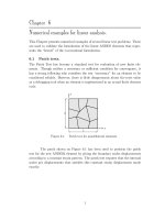
In that course we studied plates in a plane stress state, also called membrane or lamina state, which
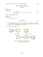
occurs if the external loads act on the plate midsurface as sketched in Figure 24.1(a). Under these

conditions the distribution of stresses and strains across the thickness may be viewed as uniform,
and the three dimensional problem can be reduced to two dimensions. If the plate displays linear
elastic behavior under the range of applied loads then we have effectively reduced the problem to
one of two-dimensional elasticity.
§24.2.1. Structural Function
In this Chapter we study plates subjected to transverse loads, that is, loads normal to its midsurface
as sketched in Figure 24.1(b). As a result of such actions the plate displacements out of its plane
and the distribution of stresses and strains across the thickness is no longer uniform. Finding those
displacements, strains and stresses is the problem of plate bending.
Plate bending components occur when plates function as shelters or roadbeds: flat roofs, bridge
and ship decks. Their primary function is to carry out lateral loads to the support by a combination
of moment and shear forces. This process is often supported by integrating beams and plates. The
beams act as stiffeners and edge members.
If the applied loads contain both loads and in-plane components, plates work simultaneously in
membrane and bending. An example where that happens is in folding plate structures common
in some industrial buildings. Those structures are composed of repeating plates that transmit roof
loads to the edge beams through a combination of bending and “arch” actions; if so all plates
experience both types of action. Such a combination is treated in finite element methods by flat
shell elements. Plates designed to resist both membrane and bending actions are sometimes called
slabs.

24–3


24–4

Chapter 24: KIRCHHOFF PLATES: FIELD EQUATIONS

z

z
(b)

(a)

y

y
x

x

Figure 24.1. A flat plate structure in: (a) plane stress or membrane state, (b) bending state.

§24.2.2. Plate Terminology
This subsection defines a plate structure in a more precise form and introduces terminology.
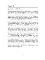
Consider first a flat surface, called the plate reference surface or simply its midsurface or midplane.
See Figure 24.2. We place the axes x and y on that surface to locate its points. The third axis, z is
taken normal to the reference surface forming a right-handed Cartesian system. Axis x and y are
placed in the midplane, forming a right-handed Rectangular Cartesian Coordinate (RCC) system.
If the plate is shown with an horizontal midsurface, as in Figure 24.2, we shall orient z upwards.
Next, imagine material normals, also called material filaments, directed along the normal to the
reference surface (that is, in the z direction) and extending h/2 above and h/2 below it. The
magnitude h is the plate thickness. We will generally allow the thickness to be a function of x, y,
that is h = h(x, y), although of course most plates used in practice are of uniform thickness because
of fabrication considerations. The end points of these filaments describe two bounding surfaces,
called the plate surfaces; the one in the +z direction is by convention called the top surface whereas
the one in the −z direction is the bottom surface.
Such a three dimensional body is called a plate if the thickness dimension h is everywhere small,
but not too small, compared to a characteristic length L c of the plate midsurface. The term “small”

is to be interpreted in the engineering sense and not in the mathematical sense. For example, h/L c
is typically 1/5 to 1/100 for most plate structures. A paradox is that an extremely thin plate, such
as the fabric of a parachute or a hot air balloon, ceases to function as a thin plate!
A plate is bent if it carries loads normal to its midsurface as shown in Figure 24.1(b). The resulting
problems of structural mechanics are called:
Inextensional bending: if the plate does not experience appreciable stretching or contractions of its
midsurface. Also called simply plate bending.
Extensional bending: if the midsurface experiences significant stretching or contraction. Also
called combined bending-stretching, coupled membrane-bending, or shell-like behavior.
The bent plate problem is reduced to two dimensions as sketched in Figure 24.2(c). The reduction
is done through a variety of mathematical models discussed next.

24–4


24–5

§24.2
Midsurface

BASIC CONCEPTS

y

(b)

Mathematical
Idealization

Plate

Γ
x

(c)

Ω

(a)
Thickness h
Material normal, also
called material filament

Figure 24.2. Idealization of plate as two-dimensional problem.

§24.2.3. Mathematical Models
The behavior of plates in the membrane state of Figure 24.1(a) is adequately covered by twodimensional continuum mechanics models. On the other hand, bent plates give rise to a wider
range of physical behavior because of possible coupling of membrane and bending actions. As
a result, several mathematical models have been developed to cover that spectrum. The more
important models are listed next.
Membrane shell model: for extremely thin plates dominated by membrane effects, such as inflatable
structures and fabrics (parachutes, sails, etc).
Von-Karman model: for very thin bent plates in which membrane and bending effects interact
strongly on account of finite lateral deflections.1 Important model for post-buckling analysis.
Kirchhoff model: for thin bent plates with small deflections, negligible shear energy and uncoupled
membrane-bending action.2
Reissner-Mindlin model: for thin and moderately thick bent plates in which first-order transverse
shear effects are considered.3 Particularly important in dynamics as well as honeycomb and composite wall constructions.
High order composite models: for detailed (local) analysis of layered composites including inter1

Th. v. K´arm´an, Festigkeistprobleme im Maschinenbau., Encyklop¨adie der Mathematischen Wissenschaften, 4/4, 311–
385, 1910.

2

¨
G. Kirchhoff, Uber
das Gleichgewicht und die Bewegung einer elastichen Scheibe, Crelles J., 40, 51-88, 1850. Also his
Vorlesungen u¨ ber Mathematischen Physik, Mechanik, 1877., translated to French by Clebsch.

3

E. Reissner, The effect of transverse shear deformation on the bending of elastic plates, J. Appl. Mech., 12, 69–77, 1945;
also E. Reissner, On bending of elastic plates, Quart. Appl. Math., 5, 55–68, 1947. Mindlin’s version, intended for
dynamics, was published in R. D. Mindlin, Influence of rotary inertia and shear on flexural vibrations of isotropic, elastic
plates, J. Appl. Mech., 18, 31–38, 1951. Timoshenko and Woinowsky-Krieger, cited in §24.5, follow A. E. Green, On
Reissner’s theory of bending of elastic plates, Quart. Appl. Math., 7, 223–228, 1949.

24–5


24–6

Chapter 24: KIRCHHOFF PLATES: FIELD EQUATIONS

θy

θy

y

Deformed
misurface

Γ

θx

w(x,y)

x

Original
misurface
x

Section y = 0

Ω

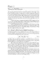
Figure 24.3. Kinematics of a Kirchhoff plate. Lateral deflection w greatly exaggerated
for visibility. In practice w << h for the Kirchhoff model to be valid.

lamina shear effects.4
Exact models: for the analysis of additional effects using three dimensional elasticity.5
The first two models are geometrically nonlinear and thus fall outside the scope of this course. The
last four models are geometrically linear in the sense that all governing equations are set up in the
reference or initially-flat configuration. The last two models are primarily used in detailed or local
stress analysis near edges, point loads or openings.
All models may incorporate other types of nonlinearities due, for example, to material behavior,
composite fracture, cracking or delamination, as well as certain forms of boundary conditions. In

this course, however, we shall look only at the linear versions. Furthermore, we shall focus attention
only on the Kirchhoff and Reissner-Mindlin plate models because these are the most commonly
global used in statics and vibrations, respectively.
§24.3. THE KIRCHHOFF PLATE
Historically the first model of thin plate bending was developed by Lagrange, Poisson and Kirchhoff.
It is known as the Kirchhoff plate model, of simply Kirchhoff plate, in honor of the German
scientist who “closed” the mathematical formulation through the variational treatment of boundary
conditions. In the finite element literature Kirchhoff plate elements are often called C 1 plate
elements because that is the continuity order nominally required for the transverse displacement
shape functions.
The Kirchhoff model is applicable to elastic plates that satisfy the following conditions.
4

See for example the book by J. N. Reddy cited in §24.5.

5

The book of Timoshenko and Woinowsky-Krieger cited in §24.5 contains a brief treatment of the exact analysis in Chapter
4.

24–6


24–7

§24.3

THE KIRCHHOFF PLATE

•

The plate is thin in the sense that the thickness h is small compared to the characteristic
length(s), but not so thin that the lateral deflection w become comparable to h.

•

The plate thickness is either uniform or varies slowly so that three-dimensional stress effects
are ignored.

•

The plate is symmetric in fabrication about the midsurface.

•

Applied transverse loads are distributed over plate surface areas of dimension h or greater.6

•

The support conditions are such that no significant extension of the midsurface develops.

We now describe the field equations for the Kirchhoff plate.
§24.3.1. Kinematic Equations
The kinematics of a Bernoulli-Euler beam is based on the assumption that plane sections remain
plane and normal to the deformed longitudinal axis. The kinematics of the Kirchhoff plate is based
on the extension of this assumption to biaxial bending:

“Material normals to the original reference surface remain straight and
normal to the deformed reference surface.”

This assumption is illustrated in Figure 24.3. Upon bending, particles that were on the midsurface
z = 0 undergo a deflection w(x, y) along z. The slopes of the midsurface in the x and y directions
are ∂w/∂ x and ∂w/∂ y. The rotations of the material normal about x and y are denoted by θx and
θ y , respectively. These are positive as per the usual rule; see Figure 24.3. For small deflections and
rotations the foregoing kinematic assumption relates these rotations to the slopes:

θx =

∂w
,
∂y

θy = −

∂w
.
∂x

(24.1)

The displacements { u x , u y , u z } of a plate particle P(x, y, z) not necessarily located on the midsurface are given by

u x = −z

6

∂w
= zθ y ,
∂x

u y = −z

∂w
= −zθx ,
∂y

u z = w.

(24.2)

The Kirchhoff model can accept point or line loads and still give reasonably good deflection and bending stress
predictions for homogeneous wall constructions. A detailed stress analysis is generally required, however, near the point
of application of the loads using more refined models.

24–7


24–8

Chapter 24: KIRCHHOFF PLATES: FIELD EQUATIONS
Bending stresses
(+ as shown)
Inplane shear stresses

Normal stresses

dy

dx
h

Top surface

z

dy

dx

y

y
dx

dy

x

σyy

σxx

σxy = σ yx

x

y

y
x

Myx

Bottom surface

Myy

Myy
Bending moments
(+ as shown)

Mxx

Mxx

Mxy

y
Mxy

x

Mxx

Myy

Mxy = Myx

x

Myx

2D view

Figure 24.4. Bending stresses and moments in a Kirchhoff plate.

The strains associated with these displacements are obtained from the elasticity equations:
ex x =
e yy =
ezz =
2ex y =
2ex z =
2e yz =

∂u x
∂x
∂u y
∂y
∂u z
∂z
∂u x
∂y
∂u x
∂z
∂u y
∂z

∂ 2w
= −z 2 = −z κx x ,
∂x

∂ 2w
= −z 2 = −z κ yy ,
∂y
∂ 2w
= −z 2 = 0,
∂z
∂u y
∂ 2w
+
= −2z
= −2z κx y ,
∂x
∂ x∂ y
∂u z
∂w ∂w
+
=−
+
= 0,
∂x
∂x
∂x
∂u z
∂w ∂w
+
=−
+
= 0.
∂y
∂y

∂y

(24.3)

Here
κx y =

∂ 2w
,
∂x2

κ yy =

∂ 2w
,
∂ y2

κx y =

∂ 2w
.
∂ x∂ y

(24.4)

are the curvatures of the deflected midsurface. It is seen that the entire displacement and strain field
are fully determined if w(x, y) is given.
REMARK 24.1

Many entry-level textbooks on plates introduce the foregoing relations gently through geometric arguments,

because students may not be familiar with 3D elasticity theory. The geometric approach has the advantage

24–8


24–9

§24.3

THE KIRCHHOFF PLATE

that the kinematic limitations of the plate bending model are more easily visualized. On the other hand the
direct approach followed here is more compact.
REMARK 24.2

Some inconsistencies of the Kirchhoff model emerge on studying (24.3). For example, the transverse shear
strains are zero. If the plate is isotropic and follows Hooke’s law, this implies σx z = σ yz = 0 and consequently
there are no transverse shear forces. But these forces appear necessarily from the equilibrium equations as
discussed in §24.3.4.
Similarly, ezz = 0 says that the plate is in plane strain whereas plane stress: σzz = 0, is a closer approximation
to the physics. For a homogeneous isotropic plate, plane strain and plane stress coalesce if and only if Poisson’s
ratio is zero. Both inconsistencies are similar to those encountered in the Bernoulli-Euler beam model.

§24.3.2. Moment-Curvature Relations
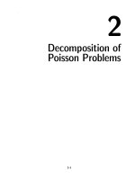
The nonzero bending strains ex x , e yy and ex y produce bending stresses σx x , σ yy and σx y as depicted
in Figure 24.4. The stress σx y is sometimes referred to as the in-plane shear stress or the bending
shear stress, to distinguish it from the transverse shear stresses σx z and σ yz studied later.
To establish the plate constitutive equations in moment-curvature form, it is necessary to make
several assumptions as to plate material and fabrication. We shall assume:
•

The plate is homogeneous, that is, fabricated of the same material through the thickness.

•

Each plate lamina z = constant is in plane stress.

•

The plate material obeys Hooke’s law for plane stress, which in matrix form is
σx x
σ yy
σx y

=

E 11
E 12
E 13

E 12
E 22
E 23

E 13
E 23
E 33

ex x
e yy

2ex y

= −z

E 11
E 12
E 13

E 12
E 22
E 23

E 13
E 23
E 33

κx x
κ yy
2κx y

.

(24.5)

The bending moments Mx x , M yy and Mx y are stress resultants with dimension of moment per unit
length, that is, force. The positive sign conventions are shown in Figure 24.4. The moments are
calculated by integrating the elementary stress couples through the thickness:
Mx x dy =
M yy d x =
Mx y dy =

M yx d x =

h/2
−h/2
h/2
−h/2
h/2
−h/2
h/2
−h/2

−σx x z dy dz,

Mx x = −

−σ yy z d x dz,

M yy = −

−σx y z dy dz,

Mx y = −

−σ yx z d x dz,

M yx = −

h/2
−h/2
h/2

−h/2
h/2
−h/2
h/2
−h/2

σx x z dz,
σ yy z dz,
(24.6)
σx y z dz,
σ yx z dz.

It will be shown later that rotational moment equilibrium implies Mx y = M yx . Consequently only
Mx x , M yy and Mx y need to be calculated. Inserting (24.5) into (24.6) and integrating, one obtains
24–9


24–10

Chapter 24: KIRCHHOFF PLATES: FIELD EQUATIONS

the moment-curvature relation
Mx x
M yy
Mx y

=

h3
12

E 11
E 12
E 13

E 12
E 22
E 23

E 13
E 23
E 33

κx x
κ yy
2κx y

=

D11
D12
D13

D12
D22
D23

D13
D23
D33

κx x
κ yy
2κx y

.

(24.7)

The Di j = E i j h 3 /12 for i, j = 1, 2, 3 are called the plate rigidity coefficients. They have dimension
of force × length. For an isotropic material of elastic modulus E and Poisson’s ratio ν, (24.7)
specializes to
κx x
1 ν
0
Mx x
(24.8)
0
M yy = D ν 1
κ yy .
Mx y
2κx y
0 0 12 (1 + ν)
Here D =

1
Eh 3 /(1
12

− ν 2 ) is called the isotropic plate rigidity.

If the bending moments Mx x , M yy and Mx y are given, the maximum values of the corresponding
in-plane stress components can be recovered from
σxmax,min
=±
x

6Mx x
,
h2

max,min
σ yy
=±

6M yy
,
h2

σxmax,min
=±
y

6Mx y
max,min
= σ yx
.
2
h

(24.9)

These max/min values occur on the plate surfaces as illustrated in Figure 24.4. Formulas (24.9) are
useful for stress design.
REMARK 24.3

For non-homogeneous plates, which are fabricated with different materials, the essential steps are the same but
the integration over the plate thickness may be significantly more laborious. (For common structures such as
reinforced concrete slabs or laminated composites, the integration process is explained in specialized books.)
If the plate fabrication is symmetric about the midsurface, inextensional bending is possible, and the end result
is a moment-curvature relation such as (24.8). If the wall fabrication is not symmetric, however, coupling
occurs between membrane and bending effects even if the plate is only laterally loaded. The Kirchhoff and
the plane stress model need to be linked to account for those effects. This coupling is examined further in
chapters dealing with shell models.

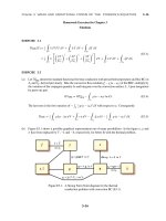
§24.3.3. Transverse Shear Forces and Stresses
The equilibrium equations derived in §24.3.4 require the presence of transverse shear forces. The
components of these forces in the { x, y } system are called Q x and Q y . These are defined as shown
in Figure 24.5. These are forces per unit of length, with physical dimensions such as N/cm or
kips/in.
Associated with these shear forces are transverse shear stresses σx z and σ yz . For a homogeneous
plate and using an equilibrium argument similar to Euler-Bernoulli beams, the stresses may be
shown to vary parabolically over the thickness, as illustrated in Figure 24.5:
σx z =

σxmax
z

4z 2
1− 2 ,

h

σ yz =

24–10

max
σ yz

4z 2
1− 2 .
h

(24.10)


24–11

§24.3
dy

dx
z

dy

dx

Parabolic distribution
across thickness

h

Top surface

THE KIRCHHOFF PLATE

Transverse shear stresses

σxz

x

y

σyz

y

y

x
Bottom surface

Qy

Qy

Qx

x

Transverse shear forces
(+ as shown)

y

Qx
2D view

x
Figure 24.5. Transverse shear forces and stresses in a Kirchhoff plate.
max
in which the peak values σxmax
and σ yz
, which occur on the midsurface z = 0, are only function
z
of x and y. Integrating over the thickness gives

Qx =

h/2
−h/2

σx z dz =

2 max
σ
3 xz

Qy =

h,

h/2
−h/2

max
σ yz dz = 23 σ yz
h,

(24.11)

If Q x and Q y are given,
=
σxmax
z

3
2

Qx
,
h

max
=
σ yz

3

2

Qy
.
h

(24.12)

As in the case of Bernoulli-Euler beams, predictions such as (24.12) must come entirely from
equilibrium analysis. The Kirchhoff plate model ignores the transverse shear energy, and in fact
predicts σx z = σ yz = 0 from the kinematic equations (24.3). Cf. Remark 24.2. In practical terms
this means that stresses (24.12) should be significantly smaller than (24.9). If they are not, the
Kirchhoff model does not apply.
§24.3.4. Equilibrium Equations
To derive the interior equilibrium equations we consider differential midsurface elements d x × dy
aligned with the { x, y } axes as illustrated in Figure 24.6. Consideration of force equilibrium along
the z direction in Figure 24.6(a) yields the shear equilibrium equation
∂ Qy
∂ Qx
+
= −q.
∂x
∂y

(24.13)

where q is the applied lateral force per unit of area. Force equilibrium along the x and y axes is
automatically satisfied and does not give additional equilibrium equations.
24–11

24–12

Chapter 24: KIRCHHOFF PLATES: FIELD EQUATIONS

z

(a)

Qx

Qy

q

Q y+
Q x+

Myy

dy

dx

x

z

(b)

∂ Qx
dx
∂x

∂ Qy
dy
∂y

y

M yx

Mxy

Mxx
dy

y

dx

Myy+

x
Mxx +

∂ M yx
∂ Mx x
dx
M yx +

dx
∂x
∂x
∂ Mx y
Mxy +
dy
∂y

∂ M yy
dy
∂y

Figure 24.6. Differential midsurface elements used to derive the
equilibrium equations of a Kirchhoff plate.

Consideration of moment equilibrium about y and x in Figure 24.6(b) yields two moment differential
equations:
∂ Mx y
∂ Mx x
+
= −Q x ,
∂x
∂y

∂ M yx
∂ M yy
+
= −Q y .
∂x
∂y

(24.14)

Moment equilibrium about z gives7
Mx y = M yx .

(24.15)

The four equilibrium equations (24.13)–(24.15) relate six fields: Mx x , Mx y , M yx , M yy , Q x and Q y .
Hence plate problems are statically indeterminate.
Eliminating Q x and Q y form (24.13) and (24.14), and setting M yx = Mx y , gives the following
moment equilibrium equation in terms of the load:
∂ 2 M yy
∂ 2 Mx y
∂ 2 Mx x
+
+
2
= q.
∂x2
∂ x∂ y
∂ y2

(24.16)

For cylindrical bending in the x direction we recover the Bernoulli-Euler beam equilibrium equation
M = q, where M ≡ Mx x and q are understood as given per unit of y width.
§24.3.5. Indicial and Matrix Forms
The foregoing field equations have been given in full Cartesian form. To facilitate reading the
existing literature and the working out the finite element formulation, the matrix and indicial forms

are displayed in Table 24.1.
7

Timoshenko’s book (cited in §24.5) unfortunately defines M yx so that Mx y = −M yx . The present convention is far more
common in recent books and agrees with the shear reciprocity σx y = σ yx of elasticity theory.

24–12


24–13

§24.3
Table 24.1

THE KIRCHHOFF PLATE

Kirchhoff Plate Field Equations in Matrix and Indicial Form

Field
eqn

Matrix
form

Indicial
form

Equation name
for plate problem

KE
CE
BE

κ = Pw
M = Dκ
PT M = q

καβ = w,αβ
Mαβ = Dαβγ δ κγ δ
Mαβ,αβ = q

Kinematic equation
Moment-curvature equation
Internal equilibrium equation

Here PT = [ ∂ 2 /∂ x 2 ∂ 2 /∂ y 2 2 ∂ 2 /∂ x∂ y ] = [ ∂ 2 /∂ x1 ∂ x1 ∂ 2 /∂ x2 ∂ x2 2 ∂ 2 /∂ x1 ∂ x2 ],
MT = [ Mx x M yy Mx y ] = [ M11 M22 M12 ],
κT = [ κx x κ yy 2κx y ] = [ κ11 κ22 2κ12 ].
Greek indices, such as α, run over 1,2 only.

§24.3.6. Skew Cuts
The preceding relations were obtained by assuming that differential elements were aligned with x
and y. Consider now the case of stress resultants acting on a plane section skewed with respect to
the x and y axes. This is illustrated in Figure 24.7, which defines notation and sign conventions.
The exterior normal n to this cut forms an angle φ with x, positive counterclockwise about z. The
tangential direction s forms an angle 90◦ + φ with x.
The bending moments and transverse shear forces defined in Figure 24.7 are related to the Cartesian
components by
Q n = Q x cφ + Q y sφ ,

Mnn = Mx x cφ2 + M yy sφ2 + 2Mx y sφ cφ ,
Mns = (M yy − Mx x )sφ cφ +

Mx y (cφ2

−

(24.17)
sφ2 ),

in which cφ = cos φ and sφ = sin φ.
These relations can be obtained directly by considering the equilibrium of the midsurface triangles
shown in the bottom of Figure 24.7. Alternatively they can be derived by transforming the wall
stresses σx x , σx y , σx y , σx z and σ yz to an oblique cut, and then integrating through the thickness.
§24.3.7. The Strong Form Diagram
Figure 24.8 shows the Strong Form diagram for the field equations of the Kirchhoff plate.
The boundary conditions are omitted since those are treated in the next Chapter.

24–13


24–14

Chapter 24: KIRCHHOFF PLATES: FIELD EQUATIONS

Parabolic distribution
across thickness

z
dy

dx ds

dx ds

s
y
n

σnz

φ

x

z

Top surface

Stresses σnn and σns
are + as shown

z

dx

ds

dy

φ

y
n

(b)

s

n
φ
dy

n

n
Mns

Mxx

x

Qn

ds

φ

x
y

y
Qy

y

σns

y
s

(a)

s

s
σnn

x

dy

x

ds

Mxy

φ

Mnn

dy
dx

dx

Myy

Qx

Myx

Figure 24.7. Skew plane sections in Kirchhoff plate.

§24.4. *THE BIHARMONIC EQUATION
Consider a homogeneous isotropic plate of constant rigidity D. Elimination of the bending moments and
curvatures from the field equations yields the famous equation for thin plates, first derived by Lagrange8
D∇ 4 w = D∇ 2 ∇ 2 w = q,
in which
∇4 ≡

∂4
∂4
∂4
+
2
+
,
∂x4

∂ x 2∂ y2
∂ y4

(24.18)

(24.19)

is the biharmonic operator. Thus, under the foregoing constitutive and fabrication assumptions the plate
deflection w(x, y) satisfies a non-homogeneous biharmonic equation. If the lateral load q vanishes, as happens
with plates loaded only on their boundaries, the deflection w satisfies the homogeneous biharmonic equation.
The biharmonic equation is the analog of the Bernoulli-Euler beam equation for uniform bending rigidity E I :
E I w I V = q, where w I V = d 4 w/d x 4 . Equation (24.18) was the basis of much of the early work in plates,
both analytical and numerical (the latter by either finite difference or Galerkin methods). After the advent of
finite elements it is largely a mathematical curiosity.
§24.5. BIBLIOGRAPHY
There is not shortage of material on plates. The problem is one of selection. Some of the best known English
textbooks and monographs are listed below. Only books examined by the writer are commented upon. Others
are simply listed. Emphasis is on technology oriented books of interest to engineers.
S. Ambartsumyan, Theory of Anisotropic Plates: Strength, Stability, and Vibrations, Hemisphere Pubs. Corp.,
1991
8

Never published; found posthumously in his Notes (1813).

24–14


24–15

§24.5 BIBLIOGRAPHY

Lateral
load
q

Deflection
w

Kinematic

κ=Pw
in Ω

Equilibrium

PT M = q
in Ω

Γ
Ω

Constitutive

Curvatures
κ

M=Dκ
in Ω

Bending

moments
M

Figure 24.8. Strong Form diagram of the field equations of the
Kirchhoff plate. Boundary condition links omitted.
C. R. Calladine, Engineering Plasticity, Pergamon Press, 1969. A textbook containing a brief treatment of
plastic behavior of homogeneous (metal) plates. Many exercises, well written.
L. H. Donnell, Beams, Plates and Shells, McGraw-Hill, 1976. Unlike Timoshenko, largely obsolete.
D. J. Gorman, Vibration Analysis of Plates by the Superposition Method, World Scientific Pub. Co, 1999
R. Hussein, Composite Panels and Plates: Analysis and Design, Technomic, Lancaster, PA, 1986.
S. G. Letnitskii, Theory of Elasticity of an Anisotropic Elastic Body, Holden-Day, 1963. Translated from
Russian. See comments for next one.
S. G. Letnitskii, Anisotropic Plates, Gordon and Breach, 1968. Translated from Russian. One of the earliest
monographs devoted to the title subject. Focus is on analytical solutions of tractable problems of anisotropic
plates.9
K. M. Liew et al. (eds.), Vibration of Mindlin Plates: Programming the P-Version Ritz Method, Elsevier
Science Ltd, 1998.
F. F. Ling (ed.), Vibrations of Elastic Plates : Linear and Nonlinear Dynamical Modeling of Sandwiches,
Laminated Composites, and Piezoelectric Layers, Springer-Verlag, New York, 1995.
A. E. H. Love, Theory of Elasticity, Cambridge, 4th ed 1927, still reprinted as a Dover book. A classical
(late XIX century) treatment of elasticity by a renowned applied mathematician contains several sections on
thin plates. Material and notation is outdated. Don’t expect any physical insight; Love has no interest in
engineering applications. Useful for tracing historical references to specific problems.
P. G. Lowe, Basic Principles of Plate Theory, Surrey Univ. Press, Blackie Group, London, 1982. An
elementary treatment of plate mechanics that covers a lot of ground, including plastic and optimal design, in
175 pages. Appropriate for supplementary reading in a senior level course.
L. S. D. Morley, Skew Plates and Structures, Pergamon Press, 1963. This tiny monograph was motivated by
the increasing importance of skew shapes in high speed aircraft after WWII. Compact and well written, still
worth consulting for benchmarks.
J. N. Reddy, Mechanics of Laminated Composite Plates, CRC Press, Boca Raton, FL, 1997. Good coverage

of methods for composite wall constructions.
9

The advent of finite elements has made the distinction between isotropic and anisotropic plates unimportant from a
computational viewpoint.

24–15


Chapter 24: KIRCHHOFF PLATES: FIELD EQUATIONS

24–16

W. Soedel, Vibrations of Plates and Shells, Marcel Dekker, 1993.
R. Szilard, Theory and Analysis of Plates, Prentice-Hall, 1974. A massive work (710 pages) similar in level
to Timoshenko’s but covering more ground: numerical methods, dynamics, vibration and stability analysis.
Although intended as a graduate textbook it contains no exercises, which detracts from its usefulness. The
treatment of numerical methods is obsolete, with many pages devoted to finite difference methods in vogue
before 1960.
S. P. Timoshenko and S. Woinowsky-Krieger, Theory of Plates and Shells, McGraw-Hill, New York, 2nd
edition, 1959. A classical reference book. Not a textbook (it lacks exercises) but case-by-case driven. It is
quintaessential Timoshenko: a minimum of generalities and lots of examples. The title is a bit misleading:
only shells of special geometries are dealt with, in 3 chapters out of 16. As for plates, the emphasis is on linear
static problems using the Kirchhoff model. There are only two chapters treating moderately large deflections,
one with the von Karman model. There is no treatment of buckling or vibration, which are covered in other
Timoshenko books.10 The reader will find no composite walls, only one chapter on orthotropic plates (called
“anisotropic” in the book) and a brief description of the Reissner-Mindlin model, which had appeared in
between the 1st and 2nd editions. Despite these shortcomings it is still the reference book to have for solution
of specific plate problems. The physical insight is unmatched. Old-fashioned full notation is used (no matrices,
vectors or tensors). Strangely, this long-windedness fits nicely with the deliberate pace of engineering before

computers, where understanding of the physics was more important than numbers. The vast compendium of
solutions comes handy when checking FEM codes, and for preliminary design work. Exhaustive reference
source for all work before 1959.
J. K. Whitney, Structural Analysis of Laminated Anisotropic Plates, Technomic Pubs Co, Lancaster, PA, 1987.
Expanded version of an 1970 book by Ashton and Whitney. Concentrates on layered composite and sandwich
wall constructions of interest in aircraft structures.
R. H. Wood, Plastic Analysis of Slabs and Plates, Thames and Hudson, 1961. Focuses on plastic analysis
of reinforced concrete plates by yield line methods. Long portions are devoted to the author’s research and
supporting experimental work. Oriented to civil engineers.
The well known handbook by Roark contains chapters collecting specific solutions of plate statics and vibration.
For general books on composite materials and their use in aerospace, civil, marine, and mechanical engineering,
a web search on new and used titles is recommended.

10

In the companion volumes Vibrations of Engineering Structures and Theory of Elastic Stability.

24–16


24–17

Exercises

Homework Exercises for Chapter 24
Kirchhoff Plates: Field Equations

EXERCISE 24.1

[A:15] The biharmonic operator (24.19) can be written symbolically as ∇ 4 = PT WP, where W is a diagonal

weighting matrix and P is defined in Table 24.1. Find W.
EXERCISE 24.2

[A:15] Using the matrix form of the Kirchhoff plate equations given in Table 24.1, eliminate the intermediate
variables κ and M to show that the generalized form of the biharmonic plate equation (24.18) is PT DP w = q.
This form is valid for anisotropic plates of variable thickness.
EXERCISE 24.3

[A:15] Rewrite PT DP w = q in indicial notation, assuming that D is constant over the plate.
EXERCISE 24.4

[A:20] Rewrite PT DP w = q in glorious full form in Cartesian coordinates, assuming that D is constant over
the plate.
EXERCISE 24.5

[A:20] Express the rotations θn and θs about the normal and tangential directions, respectively, in terms of θx ,
θ y and the angle φ defined in Figure 24.7.

24–17