Machine learning for developers uplift your regular applications with the power of statistics, analytics, and machine learning
Bạn đang xem bản rút gọn của tài liệu. Xem và tải ngay bản đầy đủ của tài liệu tại đây (24 MB, 234 trang )
Contents
1: Introduction - Machine Learning and Statistical Science
b'Chapter 1: Introduction - Machine Learning and Statistical Science'
b'Machine learning in the bigger picture'
b'Tools of the trade\xe2\x80\x93programming language and libraries'
b'Basic mathematical concepts'
b'Summary'
2: The Learning Process
b'Chapter 2: The Learning Process'
b'Understanding the problem'
b'Dataset definition and retrieval'
b'Feature engineering'
b'Dataset preprocessing'
b'Model definition'
b'Loss\xc2\xa0function definition'
b'Model fitting and evaluation'
b'Model implementation and results interpretation'
b'Summary'
b'References'
3: Clustering
b'Chapter 3: Clustering'
b'Grouping as a human activity'
b'Automating the clustering process'
b'Finding a common center - K-means'
b'Nearest neighbors'
b'K-NN sample implementation'
b'Summary'
b'References'
4: Linear and Logistic Regression
b'Chapter 4: Linear and Logistic Regression'
b'Regression analysis'
b'Linear regression'
b'Data exploration and linear regression in practice'
b'Logistic regression'
b'Summary'
b'References'
5: Neural Networks
b'Chapter 5: Neural Networks'
b'History of neural models'
b'Implementing a simple function with a single-layer perceptron'
b'Summary'
b'References'
6: Convolutional Neural Networks
b'Chapter 6: Convolutional Neural Networks'
b'Origin of convolutional neural networks'
b'Deep neural networks'
b'Deploying a deep neural network with Keras'
b'Exploring a convolutional model with Quiver'
b'References'
b'Summary'
7: Recurrent Neural Networks
b'Chapter 7: Recurrent Neural Networks'
b'Solving problems with order \xe2\x80\x94\xc2\xa0RNNs'
b'LSTM'
b'Univariate time series prediction with energy consumption data'
b'Summary'
b'References'
8: Recent Models and Developments
b'Chapter 8: Recent Models and Developments'
b'GANs'
b'Reinforcement learning'
b'Basic RL techniques: Q-learning'
b'References'
b'Summary'
9: Software Installation and Configuration
b'Chapter 9: Software Installation and Configuration'
b'Linux installation'
b'macOS X environment installation'
b'Windows installation'
b'Summary'
Chapter 1. Introduction - Machine Learning and
Statistical Science
Machine learning has definitely been one of the most talked about fields in recent years, and for
good reason. Every day new applications and models are discovered, and researchers around the
world announce impressive advances in the quality of results on a daily basis.
Each day, many new practitioners decide to take courses and search for introductory materials so
they can employ these newly available techniques that will improve their applications. But in
many cases, the whole corpus of machine learning, as normally explained in the
literature, requires a good understanding of mathematical concepts as a prerequisite, thus
imposing a high bar for programmers who typically have good algorithmic skills but are less
familiar with higher mathematical concepts.
This first chapter will be a general introduction to the field, covering the main study areas of
machine learning, and will offer an overview of the basic statistics, probability, and calculus,
accompanied by source code examples in a way that allows you to experiment with the provided
formulas and parameters.
In this first chapter, you will learn the following topics:
What is machine learning?
Machine learning areas
Elements of statistics and probability
Elements of calculus
The world around us provides huge amounts of data. At a basic level, we are continually
acquiring and learning from text, image, sound, and other types of information surrounding us.
The availability of data, then, is the first step in the process of acquiring the skills to perform a
task.
A myriad of computing devices around the world collect and store an overwhelming amount of
information that is image-, video-, and text-based. So, the raw material for learning is clearly
abundant, and it's available in a format that a computer can deal with.
That's the starting point for the rise of the discipline discussed in this book: the study of
techniques and methods allowing computers to learn from data without being explicitly
programmed.
A more formal definition of machine learning, from Tom Mitchell, is as follows:
"A computer program is said to learn from experience E with respect to some class of tasks
T and performance measure P, if its performance at tasks in T, as measured by P, improves
with experience E."
This definition is complete, and reinstates the elements that play a role in every machine learning
project: the task to perform, the successive experiments, and a clear and appropriate performance
measure. In simpler words, we have a program that improves how it performs a task based on
experience and guided by a certain criterion.
Machine learning in the bigger picture
Machine learning as a discipline is not an isolated field—it is framed inside a wider
domain, Artificial Intelligence (AI). But as you can guess, machine learning didn't appear from
the void. As a discipline it has its predecessors, and it has been evolving in stages of increasing
complexity in the following four clearly differentiated steps:
1. The first model of machine learning involved rule-based decisions and a simple level of
data-based algorithms that includes in itself, and as a prerequisite, all the possible
ramifications and decision rules, implying that all the possible options will be hardcoded
into the model beforehand by an expert in the field. This structure was implemented in the
majority of applications developed since the first programming languages appeared in
1950. The main data type and function being handled by this kind of algorithm is the
Boolean, as it exclusively dealt with yes or no decisions.
2. During the second developmental stage of statistical reasoning, we started to let the
probabilistic characteristics of the data have a say, in addition to the previous choices set
up in advance. This better reflects the fuzzy nature of real-world problems, where outliers
are common and where it is more important to take into account the nondeterministic
tendencies of the data than the rigid approach of fixed questions. This discipline adds to
the mix of mathematical tools elements of Bayesian probability theory. Methods
pertaining to this category include curve fitting (usually of linear or polynomial), which
has the common property of working with numerical data.
3. The machine learning stage is the realm in which we are going to be working throughout
this book, and it involves more complex tasks than the simplest Bayesian elements of the
previous stage. The most outstanding feature of machine learning algorithms is that they
can generalize models from data but the models are capable of generating their own
feature selectors, which aren't limited by a rigid target function, as they are generated and
defined as the training process evolves. Another differentiator of this kind of model is that
they can take a large variety of data types as input, such as speech, images, video, text, and
other data susceptible to being represented as vectors.
4. AI is the last step in the scale of abstraction capabilities that, in a way, include all previous
algorithm types, but with one key difference: AI algorithms are able to apply the learned
knowledge to solve tasks that had never been considered during training. The types of data
with which this algorithm works are even more generic than the types of data supported by
machine learning, and they should be able, by definition, to transfer problem-solving
capabilities from one data type to another, without a complete retraining of the model. In
this way, we could develop an algorithm for object detection in black and white images
and the model could abstract the knowledge to apply the model to color images.
In the following diagram, we represent these four stages of development towards real AI
applications:
Types of machine learning
Let's try to dissect the different types of machine learning project, starting from the grade of
previous knowledge from the point of view of the implementer. The project can be of the
following types:
Supervised learning: In this type of learning, we are given a sample set of real data,
accompanied by the result the model should give us after applying it. In statistical terms,
we have the outcome of all the training set experiments.
Unsupervised learning: This type of learning provides only the sample data from the
problem domain, but the task of grouping similar data and applying a category has no
previous information from which it can be inferred.
Reinforcement learning: This type of learning doesn't have a labeled sample set and has a
different number of participating elements, which include an agent, an environment, and
learning an optimum policy or set of steps, maximizing a goal-oriented approach by using
rewards or penalties (the result of each attempt).
Take a look at the following diagram:
Main areas of Machine Learning
Grades of supervision
The learning process supports gradual steps in the realm of supervision:
Unsupervised Learning doesn't have previous knowledge of the class or value of any
sample, it should infer it automatically.
Semi-Supervised Learning, needs a seed of known samples, and the model infers the
remaining samples class or value from that seed.
Supervised Learning: This approach normally includes a set of known samples, called
training set, another set used to validate the model's generalization, and a third one, called
test set, which is used after the training process to have an independent number of samples
outside of the training set, and warranty independence of testing.
In the following diagram, depicts the mentioned approaches:
Graphical depiction of the training techniques for Unsupervised, Semi-Supervised and
Supervised Learning
Supervised learning strategies - regression versus classification
This type of learning has the following two main types of problem to solve:
Regression problem: This type of problem accepts samples from the problem domain
and, after training the model, minimizes the error by comparing the output with the real
answers, which allows the prediction of the right answer when given a new unknown
sample
Classification problem: This type of problem uses samples from the domain to assign a
label or group to new unknown samples
Unsupervised problem solving–clustering
The vast majority of unsupervised problem solving consist of grouping items by looking at
similarities or the value of shared features of the observed items, because there is no certain
information about the apriori classes. This type of technique is called clustering.
Outside of these main problem types, there is a mix of both, which is called semi-supervised
problem solving, in which we can train a labeled set of elements and also use inference to assign
information to unlabeled data during training time. To assign data to unknown entities, three
main criteria are used—smoothness (points close to each other are of the same class), cluster
(data tends to form clusters, a special case of smoothness), and manifold (data pertains to a
manifold of much lower dimensionality than the original domain).
Tools of the trade–programming language and
libraries
As this book is aimed at developers, we think that the approach of explaining the mathematical
concepts using real code comes naturally.
When choosing the programming language for the code examples, the first approach was to use
multiple technologies, including some cutting-edge libraries. After consulting the community, it
was clear that a simple language would be preferable when explaining the concepts.
Among the options, the ideal candidate would be a language that is simple to understand, with
real-world machine learning adoption, and that is also relevant.
The clearest candidate for this task was Python, which fulfils all these conditions, and especially
in the last few years has become the go-to language for machine learning, both for newcomers
and professional practitioners.
In the following graph, we compare the previous star in the machine learning programming
language field, R, and we can clearly conclude the huge, favorable tendency towards using
Python. This means that the skills you acquire in this book will be relevant now and in the
foreseeable future:
Interest graph for R and Python in the Machine Learning realm.
In addition to Python code, we will have the help of a number of the most well-known numerical,
statistical, and graphical libraries in the Python ecosystem, namely pandas, NumPy, and
matplotlib. For the deep neural network examples, we will use the Keras library, with
TensorFlow as the backend.
The Python language
Python is a general-purpose scripting language, created by the Dutch programmer Guido Van
Rossum in 1989. It possesses a very simple syntax with great extensibility, thanks to its
numerous extension libraries, making it a very suitable language for prototyping and general
coding. Because of its native C bindings, it can also be a candidate for production deployment.
The language is actually used in a variety of areas, ranging from web development to scientific
computing, in addition to its use as a general scripting tool.
The NumPy library
If we had to choose a definitive must-use library for use in this book, and a non-trivial
mathematical application written in Python, it would have to be NumPy. This library will help us
implement applications using statistics and linear algebra routines with the following
components:
A versatile and performant N-dimensional array object
Many mathematical functions that can be applied to these arrays in a seamless manner
Linear algebra primitives
Random number distributions and a powerful statistics package
Compatibility with all the major machine learning packages
Note
The NumPy library will be used extensively throughout this book, using many of
its primitives to simplify the concept explanations with code.
The matplotlib library
Data plotting is an integral part of data science and is normally the first step an analyst performs
to get a sense of what's going on in the provided set of data.
For this reason, we need a very powerful library to be able to graph the input data, and also to
represent the resulting output. In this book, we will use Python's matplotlib library to describe
concepts and the results from our models.
What's matplotlib?
Matplotlib is an extensively used plotting library, especially designed for 2D graphs. From this
library, we will focus on using the pyplot module, which is a part of the API of matplotlib and
has MATLAB-like methods, with direct NumPy support. For those of you not familiar with
MATLAB, it has been the default mathematical notebook environment for the scientific and
engineering fields for decades.
The method described will be used to illustrate a large proportion of the concepts involved, and
in fact, the reader will be able to generate many of the examples in this book with just these two
libraries, and using the provided code.
Pandas
Pandas complements the previously mentioned libraries with a special structure, called
DataFrame, and also adds many statistical and data mangling methods, such as I/O, for many
different formats, such as slicing, subsetting, handling missing data, merging, and reshaping,
among others.
The DataFrame object is one of the most useful features of the whole library, providing a special
2D data structure with columns that can be of different data types. Its structure is very similar to
a database table, but immersed in a flexible programming runtime and ecosystem, such as SciPy.
These data structures are also compatible with NumPy matrices, so we can also apply highperformance operations to the data with minimal effort.
SciPy
SciPy is a stack of very useful scientific Python libraries, including NumPy, pandas, matplotlib,
and others, but it also the core library of the ecosystem, with which we can also perform many
additional fundamental mathematical operations, such as integration, optimization, interpolation,
signal processing, linear algebra, statistics, and file I/O.
Jupyter notebook
Jupyter is a clear example of a successful Python-based project, and it's also one of the most
powerful devices we will employ to explore and understand data through code.
Jupyter notebooks are documents consisting of intertwined cells of code, graphics, or formatted
text, resulting in a very versatile and powerful research environment. All these elements are
wrapped in a convenient web interface that interacts with the IPython interactive interpreter.
Once a Jupyter notebook is loaded, the whole environment and all the variables are in memory
and can be changed and redefined, allowing research and experimentation, as shown in the
following screenshot:
Jupyter notebook
This tool will be an important part of this book's teaching process, because most of the Python
examples will be provided in this format. In the last chapter of the book, you will find the full
installation instructions.
Note
After installing, you can cd into the directory where your notebooks reside, and
then call Jupyter by typing jupyter notebook
Basic mathematical concepts
As we saw in the previous sections, this main target audience of the book is developers who want
to understand machine learning algorithms. But in order to really grasp the motivations and
reason behind them, it's necessary to review and build all the fundamental reasoning, which
includes statistics, probability, and calculus.
We will first start with some of the fundamentals of statistics.
Statistics - the basic pillar of modeling uncertainty
Statistics can be defined as a discipline that uses data samples to extract and support conclusions
about larger samples of data. Given that machine learning comprises a big part of the study of the
properties of data and the assignment of values to data, we will use many statistical concepts to
define and justify the different methods.
Descriptive statistics - main operations
In the following sections, we will start defining the fundamental operations and measures of the
discipline of statistics in order to be able to advance from the fundamental concepts.
Mean
This is one of the most intuitive and most frequently used concepts in statistics. Given a set of
numbers, the mean of that set is the sum of all the elements divided by the number of elements in
the set.
The formula that represents the mean is as follows:
Although this is a very simple concept, we will write a Python code sample in which we will
create a sample set, represent it as a line plot, and mark the mean of the whole set as a line,
which should be at the weighted center of the samples. It will serve as an introduction to Python
syntax, and also as a way of experimenting with Jupyter notebooks:
import matplotlib.pyplot as plt #Import the plot library
def mean(sampleset): #Definition header for the mean function
total=0
for element in sampleset:
total=total+element
return total/len(sampleset)
myset=[2.,10.,3.,6.,4.,6.,10.] #We create the data set
mymean=mean(myset) #Call the mean funcion
plt.plot(myset) #Plot the dataset
plt.plot([mymean] * 7) #Plot a line of 7 points located on the mean
This program will output a time series of the dataset elements, and will then draw a line at the
mean height.
As the following graph shows, the mean is a succinct (one value) way of describing the tendency
of a sample set:
In this first example, we worked with a very homogeneous sample set, so the mean is very
informative regarding its values. But let's try the same sample with a very dispersed sample set
(you are encouraged to play with the values too):
Variance
As we saw in the first example, the mean isn't sufficient to describe non-homogeneous or very
dispersed samples.
In order to add a unique value describing how dispersed the sample set's values are, we need to
look at the concept of variance, which needs the mean of the sample set as a starting point, and
then averages the distances of the samples from the provided mean. The greater the variance, the
more scattered the sample set.
The canonical definition of variance is as follows:
Let's write the following sample code snippet to illustrate this concept, adopting the previously
used libraries. For the sake of clarity, we are repeating the declaration of the mean function:
import math #This library is needed for the power operation
def mean(sampleset): #Definition header for the mean function
total=0
for element in sampleset:
total=total+element
return total/len(sampleset)
def variance(sampleset): #Definition header for the mean function
total=0
setmean=mean(sampleset)
for element in sampleset:
total=total+(math.pow(element-setmean,2))
return total/len(sampleset)
myset1=[2.,10.,3.,6.,4.,6.,10.] #We create the data set
myset2=[1.,-100.,15.,-100.,21.]
print "Variance of first set:" + str(variance(myset1))
print "Variance of second set:" + str(variance(myset2))
The preceding code will generate the following output:
Variance of first set:8.69387755102
Variance of second set:3070.64
As you can see, the variance of the second set was much higher, given the really dispersed
values. The fact that we are computing the mean of the squared distance helps to really outline
the differences, as it is a quadratic operation.
Standard deviation
Standard deviation is simply a means of regularizing the square nature of the mean square used
in the variance, effectively linearizing this term. This measure can be useful for other, more
complex operations.
Here is the official form of standard deviation:
Probability and random variables
We are now about to study the single most important discipline required for understanding all the
concepts of this book.
Probability is a mathematical discipline, and its main occupation is the study of random events.
In a more practical definition, probability normally tries to quantify the level of certainty (or
conversely, uncertainty) associated with an event, from a universe of possible occurrences.
Events
In order to understand probabilities, we first need to define events. An event is, given an
experiment in which we perform a determined action with different possible results, a subset of
all the possible outcomes for that experiment.
Examples of events are a particular dice number appearing, and a product defect of particular
type appearing on an assembly line.
Probability
Following the previous definitions, probability is the likelihood of the occurrence of an event.
Probability is quantified as a real number between 0 and 1, and the assigned probability P
increases towards 1 when the likelihood of the event occurring increases.
The mathematical expression for the probability of the occurrence of an event is P(E).
Random variables and distributions
When assigning event probabilities, we could also try to cover the entire sample and assign one
probability value to each of the possible outcomes for the sample domain.
This process does indeed have all the characteristics of a function, and thus we will have a
random variable that will have a value for each one of the possible event outcomes. We will call
this function a random function.
These variables can be of the following two types:
Discrete: If the number of outcomes is finite, or countably infinite
Continuous: If the outcome set belongs to a continuous interval
This probability function is also called probability distribution.
Useful probability distributions
Between the multiple possible probability distributions, there are a number of functions that have
been studied and analyzed for their special properties, or the popular problems they represent.
We will describe the most common ones that have a special effect on the development of
machine learning.
Bernoulli distributions
Let's begin with a simple distribution: one that has a binary outcome, and is very much like
tossing a (fair) coin.
This distribution represents a single event that takes the value 1 (let's call this heads) with a
probability of p, and 0 (lets call this tails), with probability 1-p.
In order to visualize this, let's generate a large number of events of a Bernoulli distribution using
np
and graph the tendency of this distribution, with the following only two possible outcomes:
plt.figure()
distro = np.random.binomial(1, .6, 10000)/0.5
plt.hist(distro, 2 , normed=1)
The following graph shows the binomial distribution, through an histogram, showing the
complementary nature of the outcomes' probabilities:
Binomial distribution
So, here we see the very clear tendency of the complementing probabilities of the possible
outcomes. Now let's complement the model with a larger number of possible outcomes. When
their number is greater than 2, we are talking about a multinomial distribution:
plt.figure()
distro = np.random.binomial(100, .6, 10000)/0.01
plt.hist(distro, 100 , normed=1)
plt.show()
Take a look at the following graph:
Multinomial distribution with 100 possible outcomes
Uniform distribution
This very common distribution is the first continuous distribution that we will see. As the name
implies, it has a constant probability value for any interval of the domain.
In order to integrate to 1, a and b being the extreme of the function, this probability has the value
of 1/(b-a).
Let's generate a plot with a sample uniform distribution using a very regular histogram, as
generated by the following code:
plt.figure()
uniform_low=0.25
uniform_high=0.8
plt.hist(uniform, 50, normed=1)
plt.show()
Take look at the following graph:
Uniform distribution
Normal distribution
This very common continuous random function, also called a Gaussianfunction, can be defined
with the simple metrics of the mean and the variance, although in a somewhat complex form.
This is the canonical form of the function:
Take a look at the following code snippet:
import matplotlib.pyplot as plt #Import the plot library
import numpy as np
mu=0.
sigma=2.
distro = np.random.normal(mu, sigma, 10000)
plt.hist(distro, 100, normed=True)
plt.show()
The following graph shows the generated distribution's histogram:
Normal distribution
Logistic distribution
This distribution is similar to the normal distribution, but with the morphological difference of
having a more elongated tail. The main importance of this distribution lies in its cumulative
distribution function (CDF), which we will be using in the following chapters, and will
certainly look familiar.
Let's first represent the base distribution by using the following code snippet:
import matplotlib.pyplot as plt #Import the plot library
import numpy as np
mu=0.5
sigma=0.5
distro2 = np.random.logistic(mu, sigma, 10000)
plt.hist(distro2, 50, normed=True)
distro = np.random.normal(mu, sigma, 10000)
plt.hist(distro, 50, normed=True)
plt.show()
Take a look at the following graph:
Logistic (red) vs Normal (blue) distribution
Then, as mentioned before, let's compute the CDF of the logistic distribution so that you will see
a very familiar figure, the sigmoid curve, which we will see again when we review neural
network activation functions:
plt.figure()
logistic_cumulative = np.random.logistic(mu, sigma, 10000)/0.02
plt.hist(logistic_cumulative, 50, normed=1, cumulative=True)
plt.show()
Take a look at the following graph:
Inverse of the logistic distribution
Statistical measures for probability functions
In this section, we will see the most common statistical measures that can be applied to
probabilities. The first measures are the mean and variance, which do not differ from the
definitions we saw in the introduction to statistics.
Skewness
This measure represents the lateral deviation, or in general terms, the deviation from the center,
or the symmetry (or lack thereof) of a probability distribution. In general, if skewness is
negative, it implies a deviation to the right, and if it is positive, it implies a deviation to the left:
Take a look at the following diagram, which depicts the skewness statistical distribution:
Depiction of the how the distribution shape influences Skewness.
Kurtosis
Kurtosis gives us an idea of the central concentration of a distribution, defining how acute the
central area is, or the reverse—how distributed the function's tail is.
The formula for kurtosis is as follows:
In the following diagram, we can clearly see how the new metrics that we are learning can be
intuitively understood:
Depiction of the how the distribution shape influences Kurtosis
Differential calculus elements
To cover the minimum basic knowledge of machine learning, especially the learning algorithms
such as gradient descent, we will introduce you to the concepts involved in differential calculus.
Preliminary knowledge
Covering the calculus terminology necessary to get to gradient descent theory would take many
chapters, so we will assume you have an understanding of the concepts of the properties of the
most well-known continuous functions, such as linear, quadratic, logarithmic, and
exponential, and the concept of limit.
For the sake of clarity, we will develop the concept of the functions of one variable, and then
expand briefly to cover multivariate functions.
In search of changes–derivatives
We established the concept of functions in the previous section. With the exception of constant
functions defined in the entire domain, all functions have some sort of value dynamics. That
means that f(x1) is different than f(x2) for some determined values of x.
The purpose of differential calculus is to measure change. For this specific task, many
mathematicians of the 17th century (Leibniz and Newton were the most prominent exponents)
worked hard to find a simple model to measure and predict how a symbolically defined function
changed over time.
This research guided the field to one wonderful concept—a symbolic result that, under certain
conditions, tells you how much and in which direction a function changes at a certain point. This
is the concept of a derivative.
Sliding on the slope
If we want to measure how a function changes over time, the first intuitive step would be to take
the value of a function and then measure it at the subsequent point. Subtracting the second value
from the first would give us an idea of how much the function changes over time:
import matplotlib.pyplot as plt
import numpy as np
%matplotlib inline
def quadratic(var):
return 2* pow(var,2)
x=np.arange(0,.5,.1)
plt.plot(x,quadratic(x))
plt.plot([1,4], [quadratic(1), quadratic(4)],
plt.plot([1,4], [quadratic(1), quadratic(1)],
label="Change in x")
plt.plot([4,4], [quadratic(1), quadratic(4)],
label="Change in y")
plt.legend()
plt.plot (x, 10*x -8 )
plt.plot()
linewidth=2.0)
linewidth=3.0,
linewidth=3.0,
In the preceding code example, we first defined a sample quadratic equation (2*x2) and then
defined the part of the domain in which we will work with the arange function (from 0 to 0.5, in