The development environment

Chapter 4: The Development
Environment
Overview
Modern desktop development environments use remarkably complex translation
techniques. Source code is seldom translated directly into loadable binary images.
Sophisticated suites of tools translate the source into relocatable modules,
sometimes with and sometimes without debug and symbolic information. Complex,
highly optimized linkers and loaders dynamically combine these modules and map
them to specific memory locations when the application is executed.
It’s amazing that the process can seem so simple. Despite all this behind- the-
scenes complexity, desktop application developers just select whether they want a
free-standing executable or a DLL (Dynamic Link Library) and then click Compile.
Desktop application developers seldom need to give their development tools any
information about the hardware. Because the translation tools always generate
code for the same, highly standardized hardware environment, the tools can be
preconfigured with all they need to know about the hardware.
Embedded systems developers don’t enjoy this luxury. An embedded system runs
on unique hardware, hardware that probably didn’t exist when the development
tools were created. Despite processor advances, the eventual machine language is
never machine independent. Thus, as part of the development effort, the
embedded systems developer must direct the tools concerning how to translate
the source for the specific hardware. This means embedded systems developers
must know much more about their development tools and how they work than do
their application-oriented counterparts.
Assumptions about the hardware are only part of what makes the application
development environment easier to master. The application developer also can
safely assume a consistent run-time package. Typically, the only decision an
application developer makes about the run-time environment is whether to create
a freestanding EXE, a DLL, or an MFC application. The embedded systems
developer, by comparison, must define the entire run- time environment. At a

minimum, the embedded systems developer must decide where the various
components will reside (in RAM, ROM, or flash memory) and how they will be
packaged and scheduled (as an ISR, part of the main thread, or a task launched by
an RTOS). In smaller environments, the developer must decide which, if any, of
the standard run-time features to include and whether to invent or acquire the
associated code.
Thus, the embedded systems developer must understand more about the
execution environment, more about the development tools, and more about the
run-time package.

The Execution Environment
Although you might not need to master all of the intricacies of a given instruction
set architecture to write embedded systems code, you will need to know the
following:

 How the system uses memory, including how the processor manages
its stack
 What happens at system startup
 How interrupts and exceptions are handled
In the following sections, you’ll learn what you need to know about these issues to
work on a typical embedded system built with a processor from the Motorola
68000 (68K) family. Although the details vary, the basic concepts are similar on all
systems.

Memory Organization

The first step in coming to terms with the execution environment for a new system
is to become familiar with how the system uses memory. Figure 4.1
outlines a
memory map of a generic microprocessor, the Motorola 68K (Even though the

original 68K design is over 20 years old, it is a good architecture to use to explain
general principles).


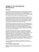
Figure 4.1: Memory map of processor.
Memory model for a 68K family processor.
Everything to the left of I/O space could be implemented as ROM. Everything to
the right of I/O space can only be implemented in RAM.
System Space
The Motorola 68K family reserves the first 1,024 memory locations (256 long
words) for the exception vector tables. Exception vectors are “hard- wired”
addresses that the processor uses to identify which code should run when it
encounters an interrupt or other exception (such as divide by zero or overflow
error). Because each vector consumes four bytes (one long word) on the 68K, this
system can support up to 256 different exception vectors.
Code Space
Above the system space, the code space stores the instructions. It makes sense to
make the system space and the code space contiguous because you would
normally place them in the same physical ROM device.
Data Space
Above the code space, the ROM data space stores constant values, such as error
messages or other string literals.
Above the data space, the memory organization becomes less regular and more
dependent on the hardware design constraints. Thus, the memory model of Figure
4.1 is only an example and is not meant to imply that it should be done that way.
Three basic areas of read/write storage (RAM) need to be identified: stack, free
memory, and heap.
The Stack
The stack is used to keep track of the current and all suspended execution
contexts. Thus, the stack contains all “live” local or automatic variables and all

function and interrupt “return addresses.” When a program calls a function, the
address of the instruction following the call (the return address) is placed on the
stack. When the called function has completed, the processor retrieves the return
address from the stack and resumes execution there. A program cannot service an
interrupt or make a function call unless stack space is available.
The stack is generally placed at the upper end of memory (see Figure 4.1
) because
the 68K family places new stack entries in decreasing memory addresses; that is,
the stack grows downwards towards the heap. Placing the stack at the “right” end
of RAM means that the logical bottom of the stack is at the highest possible RAM
address, giving it the maximum amount of room to grow downwards.
Free Memory
All statically allocated read/write variables are assigned locations in free memory.
Globals are the most common form of statically allocated variable, but C “statics”
are also placed here. Any modifiable variable with global life is stored in free
memory.
The Heap
All dynamically allocated (created by new or malloc()) objects and variables reside
in the heap. Usually, whatever memory is "left over" after allocating stack and free
memory space is assigned to the heap. The heap is usually a (sometimes complex)
linked data structure managed by routines in the compiler’s run-time package.
Many embedded systems do not use a heap.

Unpopulated Memory Space

The “break” in the center of Figure 4.1 represents available address space that
isn’t attached to any memory. A typical embedded system might have a few
megabytes of ROM-based instruction and data and perhaps another megabyte of
RAM. Because the 68K in this example can address a total of 16MB of memory,
there’s a lot of empty space in the memory map.

I/O Space

The last memory component is the memory-mapped peripheral device. In Figure
4.1, these devices reside in the I/O space area. Unlike some processors, the 68K
family doesn’t support a separate address space for I/O devices. Instead, they are
assumed to live at various addresses in the otherwise empty memory regions
between RAM and ROM. Although I’ve drawn this as a single section, you should
not expect to find all memory-mapped devices at contiguous addresses. More
likely, they will be scattered across various easy-to-decode addresses.

Detecting Stack Overflow

Notice that in Figure 4.1
on page 71, the arrow to the left of the stack space points
into the heap space. It is common for the stack to grow down, gobbling free
memory in the heap as it goes. As you know, when the stack goes too far and
begins to chew up other read/write variables, or even worse, passes out of RAM
into empty space, the system crashes. Crashes in embedded systems that are not
deterministic (such as a bug in the code) are extremely difficult to find. In fact, it
might be years before this particular defect causes a failure.
In The Art of Embedded Systems, Jack Ganssle[1] suggests that during system
development and debug, you fill the stack space with a known pattern, such as
0x5555 or 0xAA. Run the program for a while and see how much of this pattern
has been overwritten by stack operations. Then, add a safety factor (2X, perhaps)
to allow for unintended stack growth. The fact that available RAM memory could be
an issue might have an impact on the type of programming methods you use or an
influence on the hardware design.

System Startup

Understanding the layout of memory makes it easier to understand the startup
sequence. This section assumes the device’s program has been loaded into the
proper memory space — perhaps by “burning” it into erasable, programmable,
read-only memory (EPROM) and then plugging that EPROM into the system board.
Other mechanisms for getting the code into the target are discussed later.
The startup sequence has two phases: a hardware phase and a software phase.
When the RESET line is activated, the processor executes the hardware phase. The
primary responsibility of this part is to force the CPU to begin executing the
program or some code that will transfer control to the program. The first few
instructions in the program define the software phase of the startup. The software
phase is responsible for initializing core elements of the hardware and key
structures in memory.

For example, when a 68K microprocessor first comes out of RESET, it does two
things before executing any instructions. First, it fetches the address stored in the
4 bytes beginning at location 000000 and copies this address into the stack pointer
(SP) register, thus establishing the bottom of the stack. It is common for this value
to be initialized to the top of RAM (e.g., 0
X
FFFFFFFE) because the stack grows
down toward memory location 000000. Next, it fetches the address stored in the
four bytes at memory location 000004–000007 and places this 32-bit value in its
program counter register. This register always points to the memory location of
the next instruction to be executed. Finally, the processor fetches the instruction
located at the memory address contained in the program counter register and
begins executing the program.

At this point, the CPU has begun the software startup phase. The CPU is under
control of the software but is probably not ready to execute the application proper.
Instead, it executes a block of code that initializes various hardware resources and

the data structures necessary to create a complete run-time environment. This
“startup code
” is described in more detail later.

Interrupt Response Cycle
Conceptually, interrupts are relatively simple: When an interrupt signal is received,
the CPU “sets aside” what it is doing, executes the instructions necessary to take
care of the interrupt, and then resumes its previous task. The critical element is
that the CPU hardware must take care of transferring control from one task to the
other and back. The developer can’t code this transfer into the normal instruction
stream because there is no way to predict when the interrupt signal will be
received. Although this transfer mechanism is almost the same on all architectures,
TEAMFLY

Team-Fly
®

small significant differences exist among how different CPUs handle the details.
The key issues to understand are:

 How does the CPU know where to find the interrupt handling code?
 What does it take to save and restore the “context” of the main thread?
 When should interrupts be enabled?

As mentioned previously, a 68K CPU expects the first 1024 bytes of memory to
hold a table of exception vectors, that is, addresses. The first of these is the
address to load into SP during system RESET. The second is the address to load
into the program counter register during RESET. The rest of the 254 long
addresses in the exception vector table contain pointers to the starting address of
exception routines, one for each kind of exception that the 68K is capable of
generating or recognizing. Some of these are connected to the interrupts discussed
in this section, while others are associated with other anomalies (such as an
attempt to divide by zero) which may occur during normal code execution.
When a device
[1]
asserts an interrupt signal to the CPU (if the CPU is able to accept
the interrupt), the 68K will:

 Push the address of the next instruction (the return address) onto the
stack.
 Load the ISR address (vector) from the exception table into the
program counter.
 Disable interrupts.
Resume executing normal fetch–execute cycles. At this point, however, it is
fetching instructions that belong to the ISR.

This response is deliberately similar to what happens when the processor executes
a call or jump to subroutine (JSR) instruction. (In fact, on some CPUs, it is
identical.) You can think of the interrupt response as a hardware- invoked function
call in which the address of the target function is pulled from the exception vector.
To resume the main program, the programmer must terminate the ISR with a
return from subroutine (RTS) instruction, just as one would return from a function.
(Some machines require you to use a special return from interrupt [RTE, return
from exception on the 68k] instruction.)

ISRs are discussed in more detail in the next chapter
. For now, it’s enough to think
of them as hardware-invoked functions. Function calls, hardware or software, are
more complex to implement than indicated here.
[1]
In the case of a microcontroller, an external device could be internal to the chip
but exter nal to the CPU core.
Function Calls and Stack Frames

When you write a C function and assemble it, the compiler converts it to an
assembly language subroutine. The name of the assembly language subroutine is
just the function name preceded by an underscore character. For example, main()
becomes _main. Just as the C function main() is terminated by a return statement,

the assembly language version is terminated by the assembly language equivalent:
RTS.

Figure 4.2
shows two subroutines, FOO and BAR, one nested inside of the other.
The main program calls subroutine FOO which then calls subroutine BAR. The
compiler translates the call to BAR using the same mechanism as for the call to
FOO. The automatic placing and retrieval of addresses from the stack is possible
because the stack is set up as a last- in/first-out data structure. You PUSH return
addresses onto the stack and then POP them from the stack to return from the
function call.


Figure 4.2: Subroutines.

Schematic representation of the structure of an assembly-language
subroutine.

The assembly-language subroutine is “called” with a JSR assembly language
instruction. The argument of the instruction is the memory address of the start of
the subroutine. When the processor executes the JSR instruction, it automatically
places the address of the next instruction — that is, the address of the instruction
immediately following the JSR instruction — on the processor stack. (Compare this
to the interrupt response cycle discussed previously.) First the CPU decrements the
SP to point to the next available stack location. (Remember that on the 68K the SP
register grows downward in memory.) Then the processor writes the return
address to the stack (to the address now in SP).

Hint A very instructive experiment that you should be able to perform with any
embedded C compiler is to write a simple C program and compile it with a

“compile only” option. This should cause the compiler to generate an
assembly language listing file. If you open this assembly file in an editor,
you’ll see the various C statements along with the assembly language
statements that are generated. The C statements appear as comments in
the assembly language source file.
Some argue that generating assembly is obsolete. Many modern compilers skip the
assembly language step entirely and go from compiler directly to object code. If
you want to see the assembly language output of the compiler, you set a compiler
option switch that causes a disassembly of the object file to create an assembly
language source file. Thus, assembly language is not part of the process.