Modifying a Pivot Table

Modifying a Pivot Table
I
n this chapter, you’ll find solutions for problems you encounter as you make changes to your
pivot tables. One of the greatest benefits of using pivot tables is this: after you create a pivot
table, you can easily modify it. You can move the fields to a different area of the pivot table,
add or remove fields, show or hide items, and make other changes to the layout.
You may encounter problems as you change the layout, with fields that don’t behave as
expected, or features that are unavailable after you move a field. You may want to alter the
labels or values in the pivot table, and have unexpected results when you try to make the
changes. Except where noted, the problems in this chapter are based on the Sales_06.xlsx
sample workbook.
6.1. Using Report Filters: Shifting Up When Adding
Report Filters
Problem
In cell A1, above your pivot table’s Report Filter, you entered heading text for the worksheet. In
the PivotTable Field List, you dragged another field to the Report Filters area, below the exist-
ing Report Filter. When you release the mouse button, you get a warning about replacing the
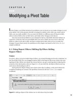
contents of the destination cells (see Figure 6-1). If you click OK, the Report Filters move up
and remove the heading in cell A1.
You’d prefer the Report Filters move down when they’re added, so they don’t delete the
worksheet heading you created. This problem is based on the RptFilters.xlsx sample
workbook.
Figure 6-1. Adding a Report Filter deletes text in cells above the pivot table.
123
CHAPTER 6
Workaround
When you add fields to the Report Filters area, Excel tries to keep the main section of the pivot
table in its current position. Existing Report Filters are pushed up to prevent the main section
from moving down. There isn’t a setting you can change to prevent this, but one of the follow-
ing workarounds may help:
• Instead of arranging the Report Filters vertically, change them to a horizontal layout, as

described in the following section.
• If you have headings on the worksheet, above the pivot table, leave a few blank rows
between them and the pivot table. If necessary, insert blank rows before adding fields
to the Report Filters area.
• If the heading information is only required for printing, move the heading text to the
Header, where it won’t be affected by changes to the pivot table layout. To insert a
Header, on the Ribbon, click the Insert tab, and then click Header & Footer in the Text
group.
6.2. Using Report Filters: Arranging Fields Horizontally
Problem
You have added several fields to the Report Filters area, and they’re pushing the pivot table
down on the worksheet. You’d like to arrange the report filters horizontally, but when you
select a report filter cell on the worksheet, and drag it to the right, you get a lengthy message
that says you cannot move a part of a PivotTable report. This problem is based on the
Horizontal.xlsx sample workbook.
Solution
By default, the Report Filters are arranged vertically above the body of the pivot table. You can
arrange the Report Filters horizontally by changing the PivotTable Options:
1. Right-click a cell in the pivot table, and then click PivotTable Options.
2. On the Layout & Format tab, click the arrow in the drop-down list beside Display Fields
in Report Filter Area, and then click Over, Then Down (see Figure 6-2).
Figure 6-2. Set the Layout options for report filters.
3. Because you selected Over, Then Down, the following drop-down list is labeled “Report
Filter Fields per Row.” Select three as the number of report filters you want across each
row, before the next row of report filters starts.
4. Click OK to close the PivotTable Options dialog box.
CHAPTER 6
■
MODIFYING A PIVOT TABLE124
How It Works

If your pivot table has many report filters, you can arrange the filters to make the most effi-
cient use of the worksheet space. The report filters should be easily accessible, not spread out
too far across the worksheet. Avoid a long column of filters above the pivot table, pushing the
pivot table body far down the worksheet.
By using the Display Fields in Report Filter Area option, you can find the best balance of
height and width for the report filter layout. The report filters can be arranged in a single col-
umn, a single row, columns of a set number of filters, or rows of a set number of filters. For
column arrangements, use the Down, Then Over option, and for row arrangements, use the
Over, Then Down option.
Down, Then Over
When a pivot table is created, the Down, Then Over option is selected by default, and the
Report Filter Fields per Column setting is zero. With these settings, the report filters are dis-
played vertically, in a single column, with no limit to the number of filters in the column.
The zero acts as a “No Limit” setting.
To limit the number of report filters in each column, change the setting from zero to
another number. For example, if you select 2, the report filters are limited to two per column
(see Figure 6-3). Once the column limit is reached, the filters move over, to start a new column.
Figure 6-3. Report filters arranged Down, Then Over, two per column
Over, Then Down
If you select the Over, Then Down option, the report filters are arranged in a row. In the
Report Filter Fields per Row option, select the number of report filters you want across each
row, before the next row of report filters starts. For example, if you select two, the report fil-
ters are limited to two per row (see Figure 6-4). Once the row limit is reached, the filters move
down, to start a new row.
■
Note
If the Report Filter Fields per Row option is set at zero, the filters are arranged in a single row.
Figure 6-4. Report filters arranged Over, Then Down, two per row
CHAPTER 6
■

MODIFYING A PIVOT TABLE 125
6.3. Using Values Fields: Changing Content in the Values Area
Problem
You use a pivot table to keep track of product samples from each category that were sent to
each sales region. You’d like to enter the sample quantities in the Values area of the pivot table,
instead of creating records in the source data. When you try to type in a cell in the Values area,
you see the error message “Cannot change this part of a PivotTable report.”
In the pivot table, the Region field is in the Row Labels area, Category is in the Column
Labels area, and Quantity is in the Values area. This problem is based on the
ChangeValues.xlsx sample workbook.
Workaround
You can’t type in cells in the Values area, with the exception of cells that contain calculated
items. For this example, you could create a calculated item with the name Samples, and a
formula of =0. Follow these steps to create a calculated item in the Category field:
1. Select one of the label cells for the Category field. If you don’t select one of these cells,
you won’t be able to create the calculated item.
2. On the Ribbon’s Options tab, in the Tools group, click Formulas, and then click Calcu-
lated Item.
3. Type Sample as the name for the calculated item.
4. Leave the default formula of =0, and then click OK.
In the pivot table, select one of the calculated item cells and type the number of samples
you sent to that region (see Figure 6-5).
Figure 6-5. Type a number in a calculated item’s cell.
■
Caution
If you clear a calculated item’s cell, you won’t be able to make any further changes to that cell.
Type a zero instead of pressing the Delete key, and you will be able to edit the cell again later.
For other cells in the Values area, unless the PivotTable settings are changed programmat-
ically, you can’t make any changes to the PivotTable values. Even if you programmatically
change a setting to allow edits to the pivot table values, the original values are restored when

the pivot table is changed or refreshed.
CHAPTER 6
■
MODIFYING A PIVOT TABLE126
6.4. Using Values Fields: Renaming Fields
Problem
When you add the Quantity field to the pivot table Values area, it’s automatically given the cus-
tom name Sum of Quantity. You’d like to change the custom name to Quantity, so it’s easier to
read and makes the column narrower. When you select the cell and type Quantity, you get an
error message: “PivotTable field name already exists.” This problem is based on the
Rename.xlsx sample workbook.
Solution
If you try to create a custom name that’s the same as a field name in the source data, you see
the error message “PivotTable field name already exists.” In this example, because one of the
fields in the source data is named Quantity, you can’t use Quantity as a custom name in the
pivot table.
However, you can avoid this problem, by adding a space character to the end of the cus-
tom name (see Figure 6-6), and it will be accepted.
Figure 6-6. Add a space character at the end of a custom name.
■
Tip
Adding a space character is a subtle change to the custom name, and would not be noticed by most
users. To help those who’ll maintain the pivot table after you’re promoted, create an Admin_Notes sheet in
the workbook. There, you can document custom name changes, calculated items, calculated fields, and
other helpful details.
6.5. Using Values Fields: Arranging Vertically
Problem
You added two fields to the Values area, and the Values fields are listed horizontally with the
Column Labels fields. You want the Values fields arranged vertically, under the Row Labels.
This will make the report narrower, and you’ll be able to print it vertically on the page. This

problem is based on the Values.xlsx sample workbook.
CHAPTER 6
■
MODIFYING A PIVOT TABLE 127
Solution
To arrange the Values fields vertically, drag the ∑ Values field in the PivotTable Field List, from
the Column Labels area to the Row Labels area (see Figure 6-7).
Figure 6-7. Move the ∑ Values field to the Row Labels area.
6.6. Using Values Fields: Fixing Source Data Number Fields
Problem
Your source data contains a column of numbers that shows the quantity for each order. You
added the Quantity field to the Values area, and the sums show zero, instead of the correct
totals. This problem is based on the FixNumbers.xlsx sample workbook.
Solution
Perhaps that column in the source data was formatted as text, before the quantities were
entered, so the numbers in the Quantity column are really text. When added to the Values
area, text cells total zero. To convert text “numbers” to real numbers, you can use one of the
techniques described in Section 5.2.
6.7. Using Values Fields: Showing Text in the Values Area
Problem
When you add the Region field to the Values area, it appears as Count of Region, instead of
showing the region names from the source data. You’d like to show the region names, so you
can create a summary report showing the region for each store. This problem is based on the
ValueText.xlsx sample workbook.
Workaround
You can’t display text fields as text in the Values area. You could add the Region field to the Row
Labels area, where the names will be displayed, and then use another field in the Values area
to show a count of the occurrences. It won’t create the exact layout you wanted, but it would
display the region and store information.
In this example, there are only two region names, so a custom number format could be

used to display the regions. Follow these steps to display the region names in the Values area:
CHAPTER 6
■
MODIFYING A PIVOT TABLE128