Sorting and Filtering Pivot Table Data

Sorting and Filtering
Pivot Table Data
A
s you analyze data in a pivot table, you may want to rearrange the items in the Row Labels
and Column Labels areas, or sort the summarized values, to focus on products that are selling
the best, or districts that are doing poorly. Sorting the labels or the values lets you move the
most important information to the top. You can also filter the labels or the values to limit the
data summarized in the pivot table.
Unless otherwise noted, the problems in this chapter are based on data in the sample file
named FoodSales.xlsx.
2.1. Sorting a Pivot Field: Sorting Row Labels
Problem
Three fields are in the Row Labels area of your pivot table: District, City, and Category, as
shown in Figure 2-1. District, the first row field, is sorted alphabetically, and you want to sort
the districts in ascending order by their total sales. The TotalSale field is in the Values area.
Sorting the row labels alphabetically or by values is simple when only one field is in the
Row Labels area, but you sometimes have problems when multiple fields exist. This problem
is based on the sample file FoodSales.xlsx.
■
Note
If a pivot table has more than one field in the Row Labels area, the field that’s last in the list is the
inner field. All the remaining row fields are outer fields. In Figure 2-1, District and City are the outer row
fields, and Category is the inner row field.
21
CHAPTER 2
Figure 2-1. District and City are the outer row fields and Category is the inner row field.
Solution
When a single field is in the Row Labels area, you can select any row label or value cell, and
click the A-Z button on the Ribbon’s Data tab to sort the labels. With multiple fields, the key to
success lies in selecting an appropriate cell before sorting.
Sorting by Labels

To sort a field alphabetically, follow these steps:
1. Right-click a row label for the field you want to sort. For example, to sort the District
field’s labels, right-click the East label.
2. Click Sort, and then click Sort A to Z.
Sorting by Values
If the values or subtotals are visible, follow these steps to sort a field’s row labels by their
values:
1. Right-click a value cell or subtotal for the field you want to sort. For example, to sort
the District field’s values, right-click the subtotal for the Central district.
2. Click Sort, and then click Sort Largest to Smallest.
Only the row labels for the selected field will be sorted. For example, if you sort the district
labels by their values, the city and category labels are unaffected. Also, the values are sorted
within their group. For example, if you sort the categories by value, the categories listed under
each city are sorted by value. As a result, the categories may appear in a different order under
each city.
Sorting by Values with Hidden Subtotals
For an outer field in the Row Labels area, subtotals may be hidden. If the subtotals are not visi-
ble, additional steps are required to sort the row labels by their values. Follow these steps to
sort a field’s row labels by their values, in ascending order:
CHAPTER 2
■
SORTING AND FILTERING PIVOT TABLE DATA22
1. Right-click a row label for the field you want to sort. For example, to sort the City field’s
labels, right-click Boston.
2. Click Sort, and then click More Sort Options.
3. Under Sort Options, select Ascending (A to Z) by.
4. From the drop-down list, select the value field by which you want to sort. In this exam-
ple, Sum of TotalSale would be the value field selected.
5. Click OK to close the Sort dialog box.
How It Works

In a pivot table, when you do an ascending sort, values are sorted in the following order:
1. Numbers (including dates, which Excel stores as numbers).
2. Text, in the following order:0123456789(space) ! “ # $ % & ( ) * , . / : ; ? @ [ \ ] ^ _ ` { |
}~+<=>ABCDEFGHIJKLMNOPQRSTUVWXYZ.
Hyphens and apostrophes are ignored, except where two items are the same except for
a hyphen. In that case, in an ascending sort, the item with the hyphen is sorted after
the similar items without the hyphen. For example, Arrowroot would be listed before
-Arrowroot.
3. Logical values (FALSE comes before TRUE).
4. Error values, such as #N/A and #NAME?. Unlike a worksheet sort, where error values
are treated equally, error values in a pivot table are sorted alphabetically.
5. Blank cells.
2.2. Sorting a Pivot Field: New Items Out of Order
Problem
Your company has just started to sell binders, in addition to its existing products, and this
morning you entered the first order for binders in your pivot table source data. The Product
field is in the Row Labels area of the pivot table, and Quantity is in the Values area.
When you refreshed the pivot table, Binders appeared at the bottom of the Product list,
instead of the top. It’s also at the bottom of the drop-down filter list for the row labels. This
makes finding the new product in the list difficult, and you’d like it sorted alphabetically with
the other products. This problem is based on the sample file
NewProduct.xlsx.
Solution
If a field’s sort setting is set for Manual sort, new items will appear at the end of the drop-down
list. This sort setting can occur if you manually rearrange the items in the Row Labels area.
Follow these steps to sort the field in ascending order:
CHAPTER 2
■
SORTING AND FILTERING PIVOT TABLE DATA 23
1. Right-click a cell in the Product field. For example, right-click the Envelopes cell.

2. Click Sort, and then click Sort A to Z.
When you sort the field, its sort setting changes from Manual to Sort Ascending or Sort
Descending. This also sorts the drop-down list, and makes it easier for users to find the items
they need.
2.3. Sorting a Pivot Field: Sorting Items Left to Right
Problem
In your pivot table, the City field is in the Column Labels area, the Product field is in the Row
Labels area, and TotalSale is in the Values area. The city names in the column headings are
sorted alphabetically.
You’re planning a new marketing campaign for bran bars, and you want to focus on the
cities with the highest sales for this product. You’d like to sort the values in the Bran row from
left to right, so the city with the highest sales for bran bars is at the left. This problem is based
on the sample file FoodSales.xlsx.
Solution
You can sort a row label by its values, left to right. In this example, the Bran product will be
sorted by its TotalSale amounts. The column heading for the city with largest amount sold will
be at the left.
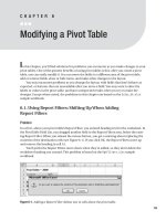
1. In the pivot table, right-click a value cell in the Bran row.
2. Click Sort, and then click More Sort Options, to open the Sort By Value dialog box.
3. Under Sort Options, select Largest to Smallest.
4. Under Sort direction, select Left to Right. In the Summary section, you can see a
description of the sort settings (see Figure 2-2).
5. Click OK to close the dialog box.
The TotalSale values for the Bran product are sorted largest to smallest, from left to right. The
City column order has changed, and New York, which has the highest Bran sales, is at the left.
Rows for other products may not be in descending order, because the column order has been
set by the Bran product.
CHAPTER 2
■
SORTING AND FILTERING PIVOT TABLE DATA24

Figure 2-2. Sort By Value dialog box
2.4. Sorting a Pivot Field: Sorting Items in a Custom Order
Problem
In your pivot table, the City field is in the Row Labels area, and you would like the cities listed
geographically instead of alphabetically. You can manually rearrange the city labels, but you
would prefer to have them sorted automatically. This problem is based on the sample file
FoodSales.xlsx.
Solution
In Excel, you can create custom lists, like the built-in lists of weekdays and months. For exam-
ple, you could create a custom list of districts, department names, or reporting categories, and
then use the custom lists to sort the items in your pivot table. This enables you to create
reports that are tailored to your needs, quickly and easily.
Creating a Custom List
The entries for the custom list can be imported from a worksheet list, or typed in the Custom
Lists dialog box. In this example, the list of cities is typed.
1. Click the Microsoft Office button, and at the bottom right, click Excel Options.
2. In the list of categories, click Popular, and in the Top Options for Working with Excel
section, click Edit Custom Lists.
3. In the Custom Lists dialog box, under Custom Lists, select NEW LIST.
CHAPTER 2
■
SORTING AND FILTERING PIVOT TABLE DATA 25
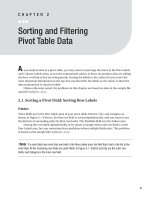
4. Click in the List Entries section, and type your list, pressing the Enter key after each
item, to separate the list items (see Figure 2-3). In this example, the list is New York,
Boston, Chicago, Seattle, Los Angeles, Dallas, Miami.
Figure 2-3. Create a custom list by typing the entries.
■
Tip
Instead of typing a list in the List Entries box, you can import the list from the worksheet by selecting
the list and clicking the Import button.

5. Click OK twice, to close the dialog boxes.
Applying the Custom Sort Order
Follow these steps to apply the custom sort order to the City field:
1. Refresh the pivot table. If the City field is set for Automatic sort, it should change to the
custom list’s sort order.
2. If the City field is currently set for manual sorting, it won’t sort according to the custom
list order. To change it to automatic sorting, right-click a city label, click Sort, and then
click Sort A to Z.
CHAPTER 2
■
SORTING AND FILTERING PIVOT TABLE DATA26
2.5. Sorting a Pivot Field: Items Won’t Sort Correctly
Problem
One of your salespeople is named Jan, and her name always appears at the top of the SalesRep
items, ahead of the names that precede it alphabetically. You can manually drag her name to
the correct position in the row labels, but you’d like to know why her name is out of order, and
how you can fix the problem. This problem is based on the sample file SalesNames.xlsx.
Solution
Jan goes to the top of the list because Excel assumes Jan means January, and is an item in one
of Excel’s built-in custom lists. Other names, such as May or June, would also go to the top of
the list, because they’re also in the custom list for months. Other words may not sort as
expected if you have created other custom lists on your computer, as described in Section 2.4.
For example, you may have created custom lists of districts or departments, and those lists
take precedence when sorting labels in a pivot table.
If you don’t want to use custom lists when sorting in a pivot table, you can change a pivot
table setting, to block their use.
■
Note
Changing the Use Custom Lists When Sorting setting affects all fields in the active pivot table, not
just a specific field.

1. Right-click a cell in the pivot table, and click PivotTable Options.
2. In the PivotTable Options dialog box, click the Totals & Filters tab.
3. In the Sorting section, remove the check mark from Use Custom Lists When Sorting
(see Figure 2-4), and then click OK.
Figure 2-4. Use Custom Lists When Sorting.
CHAPTER 2
■
SORTING AND FILTERING PIVOT TABLE DATA 27