HVAC Systems Design Handbook part 8

223
Chapter
8
Design Procedures: Part 6
Automatic Controls
8.1 Introduction
HVAC systems are sized to satisfy a set of design conditions, which
are selected to generate a maximum load. Because these design con-
ditions prevail during only a few hours each year, the HVAC equip-
ment must operate most of the time at less than rated capacity. The
function of the control system is to adjust the equipment capacity to
match the load. Automatic control, as opposed to manual control, is
preferable for both accuracy and economics; the human as a controller
is not always accurate and is expensive. A properly designed, operated,
and maintained automatic control system is accurate and will provide
economical operation of the HVAC system. Unfortunately, not all con-
trol systems are properly designed, operated, and maintained.
The purpose of this chapter is to discuss control fundamentals and
applications in a concise and understandable manner. For a yet more
detailed discussion, see the references at the end of the chapter. The
diagrams shown are ‘‘generic’’ and use symbols defined in Fig. 8.65 at
the end of the chapter.
Control systems for HVAC do not operate in a vacuum. For any air
conditioning application, first, it is necessary to have a building suit-
able for the process or comfort requirements. The best HVAC system
cannot overcome inherent deficiencies in the building. Second, the
HVAC system must be properly designed to satisfy the process or com-
fort requirements. Only when these criteria have been satisfied can a
suitable control system be implemented.
Source: HVAC Systems Design Handbook
Downloaded from Digital Engineering Library @ McGraw-Hill (www.digitalengineeringlibrary.com)

Copyright © 2004 The McGraw-Hill Companies. All rights reserved.
Any use is subject to the Terms of Use as given at the website.
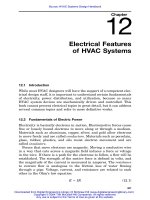
224 Chapter Eight
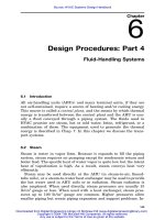
Figure 8.1
Elementary control loop.
8.2 Control Fundamentals
All control systems operate in accordance with a few basic principles.
These must be understood as background to the study of control de-
vices and system applications.
8.2.1 Control loops
Figure 8.1 illustrates a basic control loop as applied to a heating sit-
uation. The essential elements of the loop are a sensor, a controller,
and a controlled device. The purpose of the system is to maintain the
controlled variable at some desired value, called the set point. The
process plant is controlled to provide the heat energy necessary to
accomplish this. In the figure, the process plant includes the air-
handling system and heating coil, the controlled variable is the tem-
perature of the supply air, and the controlled device is the valve which
controls the flow of heat energy to the coil. The sensor measures the
air temperature and sends this information to the controller. In the
controller, the measured temperature T
m
is compared with the set
point T
s
. The difference between the two is the error signal. The con-
troller uses the error, together with one or more gain constants, to
generate an output signal that is sent to the controlled device, which
Design Procedures: Part 6
Downloaded from Digital Engineering Library @ McGraw-Hill (www.digitalengineeringlibrary.com)

Copyright © 2004 The McGraw-Hill Companies. All rights reserved.
Any use is subject to the Terms of Use as given at the website.
Design Procedures: Part 6 225
is thereby repositioned, if appropriate. This is a closed loop system,
because the process plant response causes a change in the controlled
variable, known as feedback, to which the control system can respond.
If the sensed variable is not controlled by the process plant, the control
system is open loop. Alternate terminology to the open-loop or closed
loop is the use of direct and indirect control. A directly controlled sys-
tem causes a change in position of the controlled device to achieve the
set point in the controlled variable. An indirectly controlled system
uses an input which is independent of the controlled variable to po-
sition the controlled device. An example of a direct control signal is
the use of a room thermostat to turn a space-heating device on and
off as the room temperature varies from the set point. An indirect
control signal is the use of the outside air temperature as a reference
to reset the building heating water supply temperature.
Many control systems include other elements, such as switches, re-
lays, and transducers for signal conditioning and amplification. Many
HVAC systems include several separate control loops. The apparent
complexity of any system can always be reduced to the essentials de-
scribed above.
8.2.2 Energy sources
Several types of energy are used in control systems. Most older HVAC
systems use pneumatic devices, with low-pressure compressed air at
0to20lb/in
2
gauge. Many systems are electric, using 24 to 120 V or
even higher voltages. The modern trend is to use electronic devices,
with low voltages and currents, for example, 0 to 10 V dc, 4 to 20 mA

(milliamps), or 10 to 50 mA. Hydraulic systems are sometimes used
where large forces are needed, with air or fluid pressures of 80 to 100
lb/in
2
or greater. Some control devices are self-contained, with the en-
ergy needed for the control output derived from the change of state of
the controlled variable or from the energy in the process plant. Some
systems use an electronic signal to control a pneumatic output for
greater motive force.
8.2.3 Control modes
Control systems can operate in several different modes. The simplest
is the two-position mode, in which the controller output is either on
or off. When applied to a valve or damper, this translates to open or
closed. Figure 8.2 illustrates two-position control. To avoid too rapid
cycling, a control differential must be used. Because of the inherent
time and thermal lags in the HVAC system, the operating differential
is always greater than the control differential.
Design Procedures: Part 6
Downloaded from Digital Engineering Library @ McGraw-Hill (www.digitalengineeringlibrary.com)
Copyright © 2004 The McGraw-Hill Companies. All rights reserved.
Any use is subject to the Terms of Use as given at the website.
226 Chapter Eight
Figure 8.2
Two-position control.
Figure 8.3
Modulating control.
If the output can cause the controlled device to assume any position
in its range of operation, then the system is said to modulate (Fig.
8.3). In modulating control, the differential is replaced by a throttling
range (sometimes called a proportional band), which is the range of

controller output necessary to drive the controlled device through its
full cycle (open to closed, or full speed to off).
Modulating controllers may use one mode or a combination of three
modes: proportional, integral, or derivative.
Proportional control is common in older pneumatic control systems.
This mode may be described mathematically by
Design Procedures: Part 6
Downloaded from Digital Engineering Library @ McGraw-Hill (www.digitalengineeringlibrary.com)
Copyright © 2004 The McGraw-Hill Companies. All rights reserved.
Any use is subject to the Terms of Use as given at the website.
Design Procedures: Part 6 227
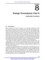
Figure 8.4
Proportional control, stable.
O ϭ A ϩ Ke (8.1)
p
where O ϭ controller output
A ϭ constant equal to controller output with no error signal
e ϭ error signal
K
p
ϭ proportional gain constant
The gain governs the change in the controller output per unit
change in the sensor input. With proper gain control, response will be
stable; i.e., when the input signal is disturbed (i.e., by a change of set
point), it will level off in a short time if the load remains constant (Fig.
8.4).
However, with proportional control, there will always be an offset—a
difference between the actual value of the controlled variable and the
set point. This offset will be greater at lower gains and lighter loads.
If the gain is increased, the offset will be less, but too great a gain

will result in instability or hunting, a continuing oscillation around
the set point (Fig. 8.5).
To eliminate the offset, it is necessary to add a second term to the
equation, called the integral mode:
O ϭ A ϩ Keϩ K
͵
edt (8.2)
pi
where K
i
ϭ integral gain constant and ͐ edtϭ integral of the error
with respect to time.
Design Procedures: Part 6
Downloaded from Digital Engineering Library @ McGraw-Hill (www.digitalengineeringlibrary.com)
Copyright © 2004 The McGraw-Hill Companies. All rights reserved.
Any use is subject to the Terms of Use as given at the website.
228 Chapter Eight
Figure 8.5
Proportional control, unstable.
Figure 8.6
Proportional plus integral control.
The integral term has the effect of continuing to increase the output
as long as the error persists, thereby driving the system to eliminate
the error, as shown in Fig. 8.6. The integral gain K
i
is a function of
time; the shorter the interval between samples, the greater the gain.
Again, too high a gain can result in instability.
The derivative mode is described mathematically by K
d

de/dt, where
de/dt is the derivative of the error with respect to time. A control mode
which includes all three terms is called PID (proportional-integral-
Design Procedures: Part 6
Downloaded from Digital Engineering Library @ McGraw-Hill (www.digitalengineeringlibrary.com)
Copyright © 2004 The McGraw-Hill Companies. All rights reserved.
Any use is subject to the Terms of Use as given at the website.
Design Procedures: Part 6 229
derivative) mode. The derivative term describes the rate of change of
the error at a point in time and therefore promotes a very rapid control
response—much faster than the normal response of an HVAC system.
Because of this it is usually preferable to avoid the use of derivative
control with HVAC. Proportional plus integral (PI) control is preferred,
and will lead to improvements in accuracy and energy consumption
when compared to proportional control alone.
Most pneumatic controllers are proportional mode only, although PI
mode is available. Most electronic controllers have all three modes
available. In a computer-based control system, any mode can be pro-
grammed by writing the proper algorithm.
8.3 Control Devices
Control devices may be grouped into the four classifications of sensors:
controllers, controlled devices, and auxiliary devices. The last group
includes relays, transducers, switches, and any other equipment
which is not part of the first three principal classifications.
8.3.1 Sensors
In HVAC work, the variables commonly encountered are the temper-
ature, humidity, pressure, and flow.
8.3.1.1 Temperature sensors.
The most common type of temperature
sensor—and historically, the first—is the bimetallic type (Fig. 8.7). The

element consists of two strips of dissimilar metals, continuously
bonded together. The two metals are selected to have very different
coefficients of expansion. When the temperature changes, one metal
expands or contracts more than the other, creating a bending action
which can be used in various ways to provide a two-position or mod-
ulating signal. A widely used configuration of the bimetal sensor is in
the form of a spiral (Fig. 8.8), allowing greater movement per unit
temperature change. Another bimetal type is the rod-and-tube sensor
(Fig. 8.9), usually inserted into a duct or pipe. The rod and tube form
the bimetal.
The bulb-and-capillary sensor (Fig. 8.10) utilizes a fluid contained
within the bulb and capillary. Various liquids and gases are used, each
suitable for a specific temperature range. The bulb may be only a few
inches long, for spot sensing, or it may be as long as 20 ft, for aver-
aging across a duct. A special application is the low-temperature
safety sensor which uses a refrigerant with a condensing temperature
of about 35ЊF. Whenever any short portion of the long bulb is exposed
to freezing temperatures, the refrigerant in that section condenses,
Design Procedures: Part 6
Downloaded from Digital Engineering Library @ McGraw-Hill (www.digitalengineeringlibrary.com)
Copyright © 2004 The McGraw-Hill Companies. All rights reserved.
Any use is subject to the Terms of Use as given at the website.
230 Chapter Eight
Figure 8.7
Bimetal temperature
sensor.
Figure 8.8
Spiral bimetal tem-
perature sensor.
Figure 8.9

Rod-and-tube temperature sensor.
Design Procedures: Part 6
Downloaded from Digital Engineering Library @ McGraw-Hill (www.digitalengineeringlibrary.com)
Copyright © 2004 The McGraw-Hill Companies. All rights reserved.
Any use is subject to the Terms of Use as given at the website.
Design Procedures: Part 6 231
Figure 8.10
Bulb-and-capillary temperature sensor.
Figure 8.11
Bellows temperature
sensor.
causing a sharp drop in the sensor pressure. This can open a two-
position switch to stop a fan and to prevent coil freeze-up.
The sealed bellows sensor (Fig. 8.11) operates on the same principle
as the bulb-and-capillary sensor. It is usually vapor-filled.
The one-pipe bleed-type sensor (Fig. 8.12) is widely used in pneu-
matic systems. Control air at 15 to 20 lb/in
2
gauge is supplied through
a small metering orifice. A flapper valve at a nozzle is modulated by
one of the previously described temperature sensors or by sensors for
flow, pressure, or humidity. As the valve varies the nozzle airflow, pres-
sure builds up or reduces in the branch line to the controller. By add-
ing appropriate springs and adjustments, this device can also be used
directly as a proportional controller.
Modern electronic control systems use some form of resistance or
capacitance temperature sensor. Widely used is the thermistor, a solid-
state device in which the electrical resistance varies as a function of
temperature. Most thermistors have a base resistance of 3000 ⍀ (or
more) at 0ЊC and a large change in resistance per degree of temper-

ature change. This makes the thermistor easy to apply, because the
resistance of wire connections (leads) is small compared to that of the
thermistor. Thermistor response is very nonlinear, but circuitry can
Design Procedures: Part 6
Downloaded from Digital Engineering Library @ McGraw-Hill (www.digitalengineeringlibrary.com)
Copyright © 2004 The McGraw-Hill Companies. All rights reserved.
Any use is subject to the Terms of Use as given at the website.
232 Chapter Eight
Figure 8.12
Bleed-type sensor controller.
be added to provide a linear signal. The principal objections to therm-
istors are (1) their tendency to drift out of calibration with time (al-
though this can be minimized with proper factory burn-in) and (2) the
problem of matching a replacement to the original thermistor (man-
ufacturers will provide ‘‘replaceable’’ devices at extra cost).
Resistance temperature detectors (RTDs) are made of fine wire
wound in a tight coil. The resistance to electric current flow varies as
a function of temperature. Various alloys are used. One alloy, with the
tradename Balco, has a base resistance of 500 ⍀ at 0ЊC. The best RTDs
are made of platinum wire. The platinum RTD has a low base
resistance—100 ⍀ at 0ЊC—so three- or four-wire leads must be used.
Platinum RTDs are very stable, showing little drift with time. Another
type of RTD is made by thin-film techniques, with a platinum film
deposited on a silicon substrate. Resistance varies with temperature,
and high base resistance can be obtained; for example, 1000 ⍀ at 0ЊC.
All these electronic sensors can be obtained in several configurations,
for room or duct or pipe mounting.
8.3.1.2 Humidity sensors.
Many hygroscopic (moisture-absorbing) ma-
terials can be used as relative-humidity sensors. Such materials ab-

sorb or lose moisture until a balance is reached with the surrounding
air. A change in material moisture content causes a dimensional
change, and this change can be used as an input signal to a controller.
Commonly used materials include human hair, wood, biwood combi-
nations similar in action to a bimetal temperature sensor, organic
films, and some fabrics, especially certain synthetic fabrics. All these
have the drawbacks of slow response and large hysteresis effects.
Design Procedures: Part 6
Downloaded from Digital Engineering Library @ McGraw-Hill (www.digitalengineeringlibrary.com)
Copyright © 2004 The McGraw-Hill Companies. All rights reserved.
Any use is subject to the Terms of Use as given at the website.
Design Procedures: Part 6 233
Temperature
sensor
Refrigeration
element
Mirror
Light
source
Power
in
Reference
photocell
Photocell
Signal
out
T
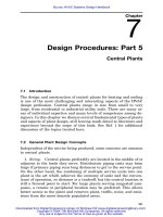
Figure 8.13
Principle of operation of chilled-mirror dew-point temperature sensor.
Their accuracy tends to be questionable unless they are frequently

calibrated. Field calibration of humidity sensors is difficult.
A different style of absorption-type dew-point sensor uses a tape
impregnated with lithium chloride and containing two wires connected
to a power supply. As moisture is absorbed by the lithium chloride, a
high-resistance electric circuit is created, which heats the system until
the system is in balance with the ambient moisture. The resulting
temperature is interpreted as the dew point. This device is accurate
when maintained at regular, frequent intervals; dirt in the system
diminishes its accuracy.
Thin-film sensors are now available which use an absorbent depos-
ited on a silicon substrate such that the resistance or capacitance var-
ies with relative humidity. These are quite accurate—ע3to5
percent—and have low maintenance requirements.
A more accurate dew point sensor is the chilled-mirror type shown
in Fig. 8.13. A light source is reflected from a stainless-steel mirror to
a photocell. The mirror is provided with a small thermoelectric cooler.
When it is cooled to the dew point, condensation begins to form on the
mirror face, the reflectivity changes, the fact is noted, and the mirror
temperature is read as the dew point temperature. The dew-point
temperature establishes the moisture content of the air. The dew-point
temperature combined with the ambient condition yields the relative
humidity (RH) by calculation. This system has a high degree of ac-
curacy, within ע1ЊF, which allows calculation of relative humidity to
an accuracy of ע2 to 3 percent. Maintenance consists of occasionally
cleaning the mirror. The device can be obtained for duct or wall mount-
ing and with circuitry to provide a dew-point temperature or a rela-
tive-humidity signal.
Design Procedures: Part 6
Downloaded from Digital Engineering Library @ McGraw-Hill (www.digitalengineeringlibrary.com)
Copyright © 2004 The McGraw-Hill Companies. All rights reserved.

Any use is subject to the Terms of Use as given at the website.
234 Chapter Eight
Figure 8.14
Diaphragm pressure sensor.
Figure 8.15
Bellows pressure sensor.
8.3.1.3 Pressure sensors.
For sensing differential pressure, some type
of diaphragm is used (Fig. 8.14). The diaphragm separates the two
halves of a closed chamber, with one of the two pressures introduced
on each half, or one-half may be open to atmosphere as a reference.
Diaphragm materials may be a flexible elastomer or thin metal, de-
pending on the use and pressure range. Sensors are available for pres-
sures ranging from a few inches of water to several thousand pounds
per square inch gauge. The flexing of the diaphragm as the pressures
change is amplified in various ways to provide a modulating signal,
which can be used for modulating or two-position control. One special
diaphragm application, called a piezometer, utilizes a crystalline struc-
ture in which the electric current flow varies as the crystal is de-
formed.
A bellows (Fig. 8.15) is a corrugated cylinder which expands or con-
tracts linearly as the pressure changes. The input pressure is always
compared to atmospheric pressure.
A bourdon tube (Fig. 8.16) is a closed semicircular tube, which tries
to straighten as the pressure is increased. This is the sensing element
in most dial pressure gauges, but it is seldom used in control devices.
Design Procedures: Part 6
Downloaded from Digital Engineering Library @ McGraw-Hill (www.digitalengineeringlibrary.com)
Copyright © 2004 The McGraw-Hill Companies. All rights reserved.
Any use is subject to the Terms of Use as given at the website.

Design Procedures: Part 6 235
Figure 8.16
Bourdon tube pressure sensor.
Note that the air velocity measured with a hot-wire anemometer
(Sec. 8.3.1.4) can be used to measure an air pressure difference be-
tween two adjacent spaces, with pressure being indicated as a function
of the airflow velocity.
8.3.1.4 Flow sensors.
In HVAC work, it is often necessary or desira-
ble to measure or detect the flow of air, water, steam, or other gases.
Several methods are available.
A sail switch is a two-position device for detecting airflow or no flow.
It consists of a lightweight sail mounted in the duct and connected to
close a switch when the sail is displaced by air movement. A similar
device, called a paddle switch, is used in piping to detect liquid flow.
These devices have a tendency to ‘‘stick’’ in the open or closed position
or to oscillate between open and closed, providing a false signal. Some
engineers believe that a more reliable flow/no-flow indication can be
obtained by reading the pressure differential across the fan or pump.
Design Procedures: Part 6
Downloaded from Digital Engineering Library @ McGraw-Hill (www.digitalengineeringlibrary.com)
Copyright © 2004 The McGraw-Hill Companies. All rights reserved.
Any use is subject to the Terms of Use as given at the website.
236 Chapter Eight
Figure 8.17
Hot-wire anemometer.
Sensing current at the motor is another way of reporting flow, but
the current sensor may not be sensitive enough to detect a broken belt
or broken coupling.
The hot-wire anemometer airflow sensor (Fig. 8.17) includes a small

electric resistance heater and a temperature sensor. The air flowing
over the heater has a cooling effect, and the air velocity is proportional
to the amount of electric energy required to maintain a reference tem-
perature. A variation of the concept imposes a fixed voltage across the
resistance, with circuitry to read the current flow which changes with
sensed temperature and with flow. Hot-wire anemometers require a
reference to neutralize the effect of changing temperature on the out-
put signal.
The pitot tube (Fig. 8.18) is a double tube, installed in a duct or pipe
so that the tip points directly into the fluid flow and therefore mea-
sures the total pressure (TP). Openings in the outer tube face at right
angles to the flow and measure static pressure (SP) only. When these
two pressures are conveyed to a differential pressure sensor or a ma-
nometer, the difference between them can be read and is equal to ve-
locity pressure (VP) from the equation
VP ϭ TP Ϫ SP (8.3)
The velocity V can then be determined from
Design Procedures: Part 6
Downloaded from Digital Engineering Library @ McGraw-Hill (www.digitalengineeringlibrary.com)
Copyright © 2004 The McGraw-Hill Companies. All rights reserved.
Any use is subject to the Terms of Use as given at the website.
Design Procedures: Part 6 237
Figure 8.18
Pitot-tube flow sensor.
V ϭ C͙VP (8.4)
where, for HVAC work, V is in feet per minute and VP is in inches of
water; C is a constant related to the density of the fluid. For standard
air, C is equal to 4005. For other than standard air, the value of C is
corrected by dividing 4005 by the square root of the new air density
ratio. For example, the air density ratio at 5000-ft elevation (with re-

spect to standard air) is 0.826. The value of C at 5000 ft is therefore
C ϭ 4005 /͙0.826 ϭ 4400
alt
The pitot tube can be used for measuring the velocity pressure of any
fluid with a known density. It is often used for measuring water flow.
The accuracy depends on the accuracy of the device being used to
measure the differential pressure.
The orifice plate (Fig. 8.19) is used for measuring the flow of all types
of fluids. In HVAC systems, it is used primarily for water and steam
flow but can also be used for airflow. The reduction of the conduit cross
section causes an increase in fluid velocity and velocity pressure,
thereby reducing the static pressure. The change in static pressure
can be measured and used to determine total flow rate
Q ϭ CA͙H (8.5)
Design Procedures: Part 6
Downloaded from Digital Engineering Library @ McGraw-Hill (www.digitalengineeringlibrary.com)
Copyright © 2004 The McGraw-Hill Companies. All rights reserved.
Any use is subject to the Terms of Use as given at the website.
238 Chapter Eight
Figure 8.19
Orifice plate flow measurement.
where Q ϭ flow rate
A ϭ cross-sectional area of conduit
H ϭ static-pressure change
C ϭ constant relating to orifice and conduit areas and fluid
density
All values must, of course, be in consistent units.
The orifice plate is simple and relatively inexpensive, and therefore
it is widely used. It creates a dynamic loss because of the abrupt con-
traction and expansion. Its accuracy falls off rapidly as flow decreases

below about 20 percent of design. (The turndown ratio is, therefore,
about 5:1.)
The dynamic losses of an orifice meter can be eliminated or de-
creased by using a venturi (Fig. 8.20), in which the area changes are
gradual. The flow equation for the venturi is
Q ϭ C͙H (8.6)
where C is a constant determined by the manufacturer and related to
size and physical characteristics.
A turbine flow meter is a small propeller mounted in the fluid stream
and connected by a gear train to a measuring / totalizing mechanism.
Design Procedures: Part 6
Downloaded from Digital Engineering Library @ McGraw-Hill (www.digitalengineeringlibrary.com)
Copyright © 2004 The McGraw-Hill Companies. All rights reserved.
Any use is subject to the Terms of Use as given at the website.
Design Procedures: Part 6 239
Figure 8.20
Venturi meter flow measurement.
The propeller speed is proportional to the fluid velocity. Because of
hysteresis and friction in the gear train, the accuracy of measurement
will vary in a nonlinear way and must be corrected for. The rotating-
vane anemometer, used for measuring airflow, is also a turbine type
of meter.
The paddle wheel type meter is turned by the flowing fluid, with
speed being proportional to velocity. This device is connected magnet-
ically to the measuring mechanism and is accurate over a wide range
of flow.
There are other ways of sensing flow rates, but those described
above are representative of HVAC use. Note that all the modulating
sensors may also be used for two-position flow detection.
8.3.2 Controllers

Controllers may be classified by the type of control action and type of
energy used for the control signal. Control action may be two-position
or modulating, with modulating control utilizing proportional, inte-
gral, or differential modes or some combination of these. Control en-
ergy sources include pneumatic, hydraulic, electric, electronic, and
self- or system-generated. The continued development of transistor
technology into microchip technology with programmable control adds
the words analog and digital to the vocabulary. Analog suggests con-
tinuous modulation of a signal by voltage or current flow, while digital
Design Procedures: Part 6
Downloaded from Digital Engineering Library @ McGraw-Hill (www.digitalengineeringlibrary.com)
Copyright © 2004 The McGraw-Hill Companies. All rights reserved.
Any use is subject to the Terms of Use as given at the website.
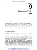
240 Chapter Eight
Figure 8.21
Bimetal two-position controller.
implies discrete or on/off. However, digital signals can approximate
analog signals by stepping a controlled device toward the open or
closed position. In fact, the accuracy of digitally controlled circuits and
devices is coming to be state of the art.
8.3.2.1 Two-position controllers.
Perhaps the simplest two-position
control is derived from the bimetal sensor, as in Fig. 8.21. The bending
action of the bimetal is used to make or break an electrical contact.
The set point is adjusted by moving the fixed contact in or out. To
provide a ‘‘snap-action make-and-break,’’ a small magnet is used. This
system has been largely superseded by one consisting of a bimetal
helical coil with a mercury switch mounted at its center (Fig. 8.22).
The switch mounting is flexible so that when the switch tilts, the mer-
cury running to one end will cause a snap action.

Virtually all the modulating-type sensors can be connected to two-
position switches of the mechanical or mercury type.
8.3.2.2 Modulating controllers.
The methods which controllers use to
determine the value of the output signal have already been discussed.
To be considered here are the various energy types used by HVAC
controllers.
By far the most common, historically, are pneumatic devices. The
principle of the nonbleed relay-type pneumatic controller is shown in
Fig. 8.23. When the sensor causes a downward movement against the
lever, the air supply valve opens and air pressure increases in the
chamber and in the output. The flexible diaphragm pushes upward
Design Procedures: Part 6
Downloaded from Digital Engineering Library @ McGraw-Hill (www.digitalengineeringlibrary.com)
Copyright © 2004 The McGraw-Hill Companies. All rights reserved.
Any use is subject to the Terms of Use as given at the website.
Design Procedures: Part 6 241
Figure 8.22
Spiral bimetal mercury switch controller.
Figure 8.23
Nonbleed relay-type controller.
against the sensor action until the air supply valve closes at some new
balance point. This is internal feedback. When the sensor action is
upward, the exhaust valve opens and some air bleeds out, reducing
the pressure to a new balance point. The gain or sensitivity to change
in the sensed variable is adjusted by varying the length of the lever
Design Procedures: Part 6
Downloaded from Digital Engineering Library @ McGraw-Hill (www.digitalengineeringlibrary.com)
Copyright © 2004 The McGraw-Hill Companies. All rights reserved.
Any use is subject to the Terms of Use as given at the website.

242 Chapter Eight
Figure 8.24
Circular rheostat.
arm. The set point is adjusted by varying the spring tension at the
sensor action. This is the classical method of building a pneumatic
controller.
The relay-type controller as shown in Fig. 8.23 uses only propor-
tional mode. It is possible to add reset functions and integral-mode
operation, although this makes a more complex device.
The bleed-type pneumatic sensor already discussed (Fig. 8.12) can
become a proportional controller if the air supply orifice is
adjustable—for gain adjustment—and the sensor-nozzle combination
is provided with a set point adjustment.
A common method of obtaining an electric modulating output em-
ploys a rheostat—a variable resistance. The rheostat may be circular
(Fig. 8.24) or linear. It forms part of an electric circuit, with current
flowing in at one end and out through the moving-arm contact. As the
arm moves in response to a modulating sensor, the amount of resis-
tance varies; therefore, the output voltage varies. The gain is a func-
tion of resistance per unit length and speed of arm travel in relation
to change in sensor input. The set point is adjusted by changing the
starting point of the moving arm.
The Wheatstone bridge (Fig. 8.25) is used in some form in most elec-
tric and electronic controllers. The principle of the bridge circuit is
that in a balanced bridge all four resistances are equal. When power
is applied, the voltages at the two output terminals are equal, and a
meter placed across those terminals shows a zero difference in poten-
tial. If one of the resistances is variable (as indicated by the arrow
across it) and is, in fact, varied, then there will be a difference in
voltage between the output terminals that is proportional to the

change in resistance. A basic bridge controller (Fig. 8.26) includes a
Design Procedures: Part 6
Downloaded from Digital Engineering Library @ McGraw-Hill (www.digitalengineeringlibrary.com)
Copyright © 2004 The McGraw-Hill Companies. All rights reserved.
Any use is subject to the Terms of Use as given at the website.
Design Procedures: Part 6 243
Figure 8.25
Wheatstone bridge.
Figure 8.26
Bridge circuit with calibration and set point.
Design Procedures: Part 6
Downloaded from Digital Engineering Library @ McGraw-Hill (www.digitalengineeringlibrary.com)
Copyright © 2004 The McGraw-Hill Companies. All rights reserved.
Any use is subject to the Terms of Use as given at the website.
244 Chapter Eight
Figure 8.27
PID controller using op amps.
change-in-resistance type of sensor, an adjustable set point resistor,
and a calibrating resistor.
Electric controllers generally operate with power supplies of 24 V
ac or more. An electronic controller usually needs a 24-V dc power
supply and provides an output signal in a range of 0 to 5 or 0 to 10 V
or 4 to 20 or 10 to 50 mA. The preferred ranges are 0 to 10 V or 4 to
20 mA. Most electronic controllers are designed around a device called
an op amp (operational amplifier). This solid-state device provides an
almost infinite amplification of an input signal. By means of appro-
priate circuitry, the op amp can add or subtract signals and provide
proportional, integral, or derivative functions. These may be combined
as shown in Fig. 8.27 to make a PID controller or any desired com-
bination thereof. For further discussion, consult a good electronics text

or Refs. 1 and 3 at the end of this chapter. For the use of a computer
as a controller, see Sec. 8.7 and Refs. 5 and 6.
The sensor and controller are often combined in one package, al-
though they serve separate functions. This package is referred to as
a stat—thermostat, humidistat, pressurestat, and flowstat. The most
common arrangement is wall-mounted in a room, but duct-mounted
stats are also frequently encountered. Electronic control systems often
use sensors wired to remotely located control boards.
8.3.3 Controlled devices
In HVAC work, controlled devices are usually valves, dampers, or mo-
tors. As previously noted, these devices may be controlled in two-
position or modulating modes.
Design Procedures: Part 6
Downloaded from Digital Engineering Library @ McGraw-Hill (www.digitalengineeringlibrary.com)
Copyright © 2004 The McGraw-Hill Companies. All rights reserved.
Any use is subject to the Terms of Use as given at the website.
Design Procedures: Part 6 245
Figure 8.28
Straight-through (two-way) control valve.
Figure 8.29a
Quick-opening (flat seat) valve.
8.3.3.1 Control valves.
A control valve (Fig. 8.28) includes a body,
within which are passages for fluid flow; a seat; and a plug. The plug
is connected to a stem, which in turn is connected to an operator.
Where it penetrates the body, the stem is provided with some kind of
seal or packing to prevent loss of fluid. Many different materials are
used for the various elements to suit the requirements of temperature,
pressure, and fluid characteristics.
The three principal plug types encountered are shown in Fig. 8.29a,

b, and c. Plug lift refers to opening the valve by lifting the plug off
the seat. The flat or quick-opening plug is suitable only for two-
position control, as shown in Fig. 8.30; a very small lift results in a
large change in the design flow rate. The linear plug is notched or
tapered in a straight line; this results in a linear or near-linear re-
Design Procedures: Part 6
Downloaded from Digital Engineering Library @ McGraw-Hill (www.digitalengineeringlibrary.com)
Copyright © 2004 The McGraw-Hill Companies. All rights reserved.
Any use is subject to the Terms of Use as given at the website.
246 Chapter Eight
Figure 8.29b
Linear (V-port) valve.
Figure 8.29c
Equal-percentage valve.
sponse to lift. The equal-percentage plug is notched or tapered in a
curved shape, resulting in an exponential response. The origin of the
curves in Fig. 8.30 is not at zero flow. This is because the valve must
be constructed with some clearance between plug and port to prevent
sticking in the closed position; when the valve is cracked open, some
minimum flow occurs. The amount of clearance, and therefore the
minimum flow rate, is a function of the valve design and quality. The
ratio of this value to 100 percent flow is known as the turndown ratio.
For a typical commercial-quality valve, this minimum flow is about
5 percent, making the turndown ratio 100:5 or 20:1. Ratios of 50:1,
100:1, or even 200:1 are available, but 20:1 is acceptable for most
HVAC work.
The equal-percentage plug is used for modulating control of water
flow because it has a lower ratio of flow increase to lift increase in the
region near to closure. This tends to offset the effect shown in Fig.
8.31. This figure shows the output of a heating coil as a function of

Design Procedures: Part 6
Downloaded from Digital Engineering Library @ McGraw-Hill (www.digitalengineeringlibrary.com)
Copyright © 2004 The McGraw-Hill Companies. All rights reserved.
Any use is subject to the Terms of Use as given at the website.
Design Procedures: Part 6 247
Figure 8.30
Flow versus plug lift in a control valve.
Figure 8.31
Coil heating capacity versus hot water flow rate.
Design Procedures: Part 6
Downloaded from Digital Engineering Library @ McGraw-Hill (www.digitalengineeringlibrary.com)
Copyright © 2004 The McGraw-Hill Companies. All rights reserved.
Any use is subject to the Terms of Use as given at the website.