(Luận văn thạc sĩ) the impact of exchange rate on trade balance between vietnam and china
Bạn đang xem bản rút gọn của tài liệu. Xem và tải ngay bản đầy đủ của tài liệu tại đây (540.91 KB, 101 trang )
UNIVERSITY OF ECONOMICS
HO CHI MINH CITY
VIETNAM
INSTITUTE OF SOCIAL STUDIES
THE HAGUE
THE NETHERLANDS
VIETNAM - NETHERLANDS
PROGRAMME FOR M.A IN DEVELOPMENT ECONOMICS
THE IMPACT OF EXCHANGE RATE ON
TRADE BALANCE BETWEEN VIETNAM AND
CHINA
BY
TRAN QUOC KHANH CUONG
MASTER OF ARTS IN DEVELOPMENT ECONOMICS
HO CHI MINH CITY, January, 2015
UNIVERSITY OF ECONOMICS
HO CHI MINH CITY
VIETNAM
INSTITUTE OF SOCIAL STUDIES
THE HAGUE
THE NETHERLANDS
VIETNAM - NETHERLANDS
PROGRAMME FOR M.A IN DEVELOPMENT ECONOMICS
THE IMPACT OF EXCHANGE RATE ON
TRADE BALANCE BETWEEN VIETNAM AND
CHINA
A thesis submitted in partial fulfilment of the requirements for the degree of
MASTER OF ARTS IN DEVELOPMENT ECONOMICS
By
TRAN QUOC KHANH CUONG
Academic Supervisor:
NGUYEN VAN NGAI
HO CHI MINH CITY, January, 2015
ACKNOWLEDGEMENT
First of all, I would like to show my deepest thanks to my supervisor, Associate
Professor, Ph. D Nguyen Van Ngai who gave scientific guidance, useful advice and
instruct me to complete this thesis.
I would like to thank Professor Chinn M. D., Professor Bahmani-Oskooee, M. and Dr.
Pham Khanh Nam who gave many useful comments during the process of doing my
thesis.
I am very grateful to the lecturers and classmates who help me to much during
studying.
Finally, I would like to give the special thanks my family who support me moral and
financial during the time I study.
i
ABSTRACTS
The goal of this research is to investigate the short term and long term relationship
between exchange rate and trade balance. Differing test such as Johansen Cointegraion
test, Vector Error Correction, Wald test etc., have been conducted. The data was
collected from International Financial Statistics (IFS), Organization for Economic
Cooperation and Development (OECD) and Asian Regional Integration Center
(ARIC). The conclusion is as follow:
• Long run relationship between real exchange rate and trade balance occurs, and
• The coefficient of real exchange rate is negative and significant.
The results implies that devaluation of currency to cure trade deficit between Vietnam
and China may not an appropriate method, for instance, the trade performanceof
Vietnam to China could deteriorate.
ii
Contents
CHAPTER 1 ................................................................................................................... 1
INTRODUCTION .......................................................................................................... 1
1.1
Problem statement .............................................................................................. 1
1.2
Research objectives ............................................................................................ 3
1.3
Research methodology ....................................................................................... 3
1.4
Structure of this thesis ........................................................................................ 3
CHAPTER 2 ................................................................................................................... 5
LITERATURE REVIEW .............................................................................................. 5
2.1
Definition of exchange rate, real exchange rate and misalignment ................... 5
2.2
Theoretical model of real exchange rate equilibrium ......................................... 6
2.2.1
Model – based approach .............................................................................. 6
2.2.2
The fundamental equilibrium exchange rate approach................................ 6
2.2.3
The purchasing power parity approach........................................................ 8
2.3
Theory of the impact of exchange rate on trade balance .................................. 10
2.3.1
Marshall – Lerner condition ...................................................................... 10
2.3.2
The J-Curve................................................................................................ 10
iii
2.4
Empirical studies .............................................................................................. 11
2.4.1
Empirical studies for the PPP approach..................................................... 11
2.4.2
Empirical studies for the BEER and the FEER ......................................... 14
2.4.3
Empirical studies of the impact of exchange rate on trade balance........... 15
2.5
Conceptual framework ..................................................................................... 20
CHAPTER 3 ................................................................................................................. 22
THE EXCHANGE RATE AND TRADE .................................................................. 22
BETWEEN VIETNAM AND CHINA ....................................................................... 22
3.1
Tendency of the exchange rate between Vietnam and China .......................... 22
3.2
Trade balance between Vietnam and China ..................................................... 23
3.3
The main commodities of import and export between Vietnam and China in
recent years ................................................................................................................. 24
3.3.1
The main commodities of export to China in recent years ........................ 24
3.3.2
Imported commodities from China ............ Error! Bookmark not defined.
CHAPTER 4 ................................................................................................................. 29
MODEL SPECITICATION AND DATA SOURCE ................................................ 29
4.1
Model for purchasing power parity approach .................................................. 29
4.2
Model for trade balance .................................................................................... 33
iv
4.3
Robustness check for VECM. .......................................................................... 37
4.3.1
Serial Correlation Test ............................................................................... 37
4.3.2
Heteroskedasticity test: .............................................................................. 37
4.3.3
Normality test: ........................................................................................... 38
4.4
Data source ....................................................................................................... 38
4.4.1
Data for PPP approach ............................................................................... 38
4.4.2
Data for trade balance ................................................................................ 39
CHAPTER 5 ................................................................................................................. 41
THE IMPACT OF EXCHANGE RATE ON TRADE BALANCE BETWEEN
VIETNAM AND CHINA .............................................................................................. 41
5.1
The estimation of real exchange rate. ............................................................... 41
5.1.1
Unit root test .............................................................................................. 41
5.1.2
Optimal lag for VECM .............................................................................. 42
5.1.3
Johansen (1988) procedure for cointegration test...................................... 45
5.1.4
The estimation of real exchange rate between Vietnam and China .......... 48
5.1.5
Robustness check for PPP model .............................................................. 49
5.2
The exchange rate misalignment between Vietnamese currency (VND) and
Chinese currency (RMB) ........................................................................................... 51
v
5.3
The impact of the exchange rate on trade balance ........................................... 53
5.3.1
Unit root test .............................................................................................. 53
5.3.2
Optimal lag for VECM .............................................................................. 55
5.3.3
Diagnostic check for every lag .................................................................. 56
5.3.4
Inverse Roots of AR characteristic polynomial ......................................... 57
5.3.5
Johansen procedure for cointegration test for the impact of exchange rate
on trade balance...................................................................................................... 57
5.3.6
The impact of exchange rate on trade balance in long run ........................ 60
5.3.7
The impact of exchange rate on trade balance in short run ....................... 60
5.3.8
Robustness Check ...................................................................................... 61
CHAPTER 6 ................................................................................................................. 66
CONCLUSIONS AND RECOMMENDATIONS ..................................................... 66
6.1
Conclusions ...................................................................................................... 66
6.2
Policy implications ........................................................................................... 67
6.3
Limitations and further researches ................................................................... 67
6.3.1
Limitations ................................................................................................. 67
6.3.2
Further researches ...................................................................................... 67
vi
LISTS OF FIGURES
Figure 2.1: J curve effect. ............................................................................................... 11
Figure 2.2: Conceptual framework of this study............................................................ 21
Figure 3.1 Nominal exchange rate between Vietnam and China, (VND/RMB) ........... 22
Figure 3.2: Trade balance between Vietnam and China (million US dollar). ............... 23
Figure 5.1: Inverse Roots of AR characteristic polynomial for PPP ............................. 44
Figure 5.2 Real exchange rate between Vietnam and China (VND/RMB) ................... 48
Figure 5.3: Normality test .............................................................................................. 51
Figure 5.3: Misalignment between VND and RMB ...................................................... 52
Figure 5.4: Inverse Roots of AR characteristic polynomial for PPP ............................. 57
Figure 5.5: Normality test for VECM model ................................................................. 63
Figure 5.6: Cumulative sum of recursive ....................................................................... 64
Figure 5.7: Cumulative sum of square of recursive ....................................................... 64
vii
LIST OF TABLES
Table 3.1: The main commodities of export to China during 2010-2013 (million USD) ........ 24
Table 3.2: The main commodities of import from China during 2010-2013, million USD..... 26
Table 4.1 Data for PPP approach .............................................................................................. 39
Table 4.2: Data for trade balance approach .............................................................................. 39
Table 5.1: Mackinon (1996) critical value. ............................................................................... 41
Table 5.2: Unit root test for PPP approach ............................................................................... 41
Table 5.3: Lag criteria for PPP approach .................................................................................. 43
Table 5.6: Wald test for Horvath – Watson procedure ............................................................. 47
Table 5.9: Unit root test on time series ..................................................................................... 54
Table 5.10: Lag selection of VECM ......................................................................................... 55
Table 5.11: Diagnostic check for every lag .............................................................................. 56
Table 5.12: Johansen cointegration test with 18 lags ............................................................... 58
Table 5.13: Cointegrating equation .......................................................................................... 59
Table 5.13: The speed of adjustment coefficient of long run ................................................... 60
Table 5.14: Wald test for the short run relationship ................................................................. 60
Table 5.16: Heteroskedasticity Test: Breusch-Pagan-Godfrey................................................. 62
viii
LISTS OF ABRREVIAION
ARDL: Autoregressive Distribution Lag
BEER: Behavior Equilibrium Exchange Rate
CPI: Consumer Price Index
FEER: Fundamental Equilibrium Exchange Rate
IIPCN: Index of Industrial Production of China
IIPVN: Index of Industrial Production of Vietnam
PPP: Purchasing Power Parity
RER: Real Exchange Rate
STAR: Smooth Transition Autoregressive
TB: Trade Balance
VECM: Vector Error Correction Model
ix
CHAPTER 1
INTRODUCTION
1.1 Problem statement
Özkan (2013) stated that real exchange rate plays an important role in the
macroeconomic such aseconomic development, sustainable growth, especially real
exchange rate plays a very important role in trade balance. Trade balance is a
component of Gross Domestic Product(GDP). GDP will increase if trade of balance
issurplus, and decrease if trade of balance isdeficit. In many recent years, Vietnam
(VN) almost has trade deficit with the rest of the world. Trade balance deficit reduces
foreign reserve, if it happens in the long term, it will lead to foreign debt. Therefore
Vietnam will lend money from abroad and pay interest to compensate for the
imbalance. However, this approach is not effective to solve this problem in long term
for Vietnam’s economy. Because this process will make budget deficit and not good
for the economy of Vietnam.
In general, there was a substantial increase in both export and import throughout the
period from 2000 to 2013. Nevertheless, this upward trend did not grow constantly. In
particular, as a result of global finance crisis, the proportion of import and export
witnessed a marginal downward trend between 2008 and 2009. At that time, balance
trade plunged into the lowest level for 11 years. However, it recovered and rose
considerably more than the previous stage.
Although export increased over and over, it was still lower than import that leaded to
trade deficit for Vietnam. Until 2012, export already kept up with the import
development, comprised nearly 115.5 billion USD that enhanced the effect and
advantage of trade balancedue to trade surplus.The most striking feature was that the
1
above surplus continually to rise and reach the highest level in 2013, amounted to 900
million USD and trade balance has the highest trade surplus.
According to general statistics office(GSO), from 2000 to 2013, the surplus of trade
balanceVietnam, US and Europehas increased since 2000. Admittedly, American and
Europe have been truly the potential market for Vietnam’s enterprises to expand export
and improve the international business profit.Nevertheless, there is a contrast sharply
of trade balance between Vietnam and Asian, especially China compared withUS or
EU. In many years, VN always has trade surplus with US and EU; nevertheless, VN
takes trade deficit with ASEAN, and especially China.
In many years, economists have concerned about the trade deficit between Vietnam
and China. And exchange rate between Vietnam and China has been considering as a
reason of trade deficit. The question is that should we depreciate our currency? This
problem is very important because exchange rate plays an important role in the
economy, especially in emergency market such as Vietnam (Stone, M.et al., 2009). It
will effect on inflation targeting whichis one of the hottest issue in Vietnam inrecent
years.
According to Marshall-Learner (ML) condition or J Curve, exchange rate plays an
important role in trade balance. Both of them state that if the currency is depreciation,
with the condition that adding the elasticity of export and import more than one, the
trade balance will increase in the long run.
As VND is appreciated, Vietnamese finds imported goods from China cheaper and
Chinese finds imported goods from Vietnam more expensive. Therefore, Vietnam has
trade deficit. Nevertheless, if VND is depreciated, an opposite effect takes place and
Vietnam takes trade surplus with China.
2
Does VND over-valuated compare with China? Does exchange rate effect to trade
balance between Vietnam and China? And does depreciation increase trade balance
between Vietnam and China?
1.2 Research objectives
Based on the problem statement, this study aims to find out:
First, estimating of the real exchange rate between Vietnam and China
Second,evaluatingof the value of Vietnamese currency against Chinese currency.
Third, examiningthe influenceof the exchange rate on trade balance between two
countries.
1.3 Research methodology
There are three procedures to solve the three objectives of this research. Firstly,
Purchasing Power Parity is used to estimate the real exchange rate between Vietnam
and China. Secondly, time trend is used to evaluateof the value of Vietnamese currency
against Chinese currency. And finally, cointegration and vector error correction is used
to estimate the impact of the exchange rate on trade balance between two countries.
1.4 Structure of this thesis
The thesis consists of five chapters which are arranged as follows:
Chapter 1 provides an overview for the trade balance of Vietnam in recent years, and
explains several reasons for choosing this topic and research objectives.
Chapter 2 is assigned to literature review. This chapter provides the theories and
empirical studies for calculating real exchange rate, the impact of exchange rate on
3
trade balance. Moreover, the conceptual framework will offer a general step to be
conducted in this thesis as well.
Chapter 3 analyzes the influence of exchange rate on trade balance between Vietnam
and China. This chapter provides an overview the bilateral trade between two
countries in general and in details.
Chapter 4 describes the methodology and data collection for this thesis. This chapter
containsempirical models that will apply for the next chapter as well as data sources.
Following chapter 4, chapter 5 presents and discusses empirical results. Econometric
results are shown and discussed to determine the real exchange rate, misalignments
between Vietnam and China. Finally, the role of exchange rate in trade balance
between Vietnam and China is covered.
Finally, with all results and analyses from previous chapters, the chapter 6 provides
recommendations for policy makers. Additionally, the last part contains limitations
and further researches as well.
4
CHAPTER 2
LITERATURE REVIEW
Before calculating misalignments, the equilibrium real exchange rate should be initially
estimated. This chapter provides two approaches for calculating equilibrium exchange
rate. The disadvantagesof each approach would be considered, then selects the suitable
approach to calculate misalignments. After that, the role of exchange rate in bilateral
trade will be examined.
2.1 Definitionof exchange rate, real exchange rate and misalignment
GÄrtner (2009) stated that exchange rate is defined either as the price of one unit
foreign currency in termsof domestic currencyor the ratio between the price of a bundle
of goods foreign and domestic.
Definition of real exchange rate (RER) is the ratio price of traded goods to non-traded
goods. The equilibrium real exchange rate (ERER) is defined as the rate price of traded
goods to non-traded goods that results from the simultaneous achievement of
equilibrium in the external sector and internal sector of a country.
The misalignment is the differencebetween real exchange rate and equilibrium
exchange rate. The misalignment implies the currency overvalued when it is positive,
otherwise the currency undervalued.
In order to calculate the misalignment, we have to calculate the equilibrium real
exchange rate (ERER). There are some methods to calculate ERER such as PPP
approach, model – based approach.
5
2.2 Theoretical model of real exchange rate equilibrium
2.2.1 Model – based approach
Model – based approach (Clark and McDonald, 1998) measures RER misalignments
based on the ERER. This is familiar with “behavior equilibrium exchange rate”
(BEER) approach and “fundamental equilibrium exchange rate” (FEER) approach.
These approaches are engines to estimate exchange rate.
2.2.2 The fundamental equilibrium exchange rate approach
Clark and McDonald (1998) said that the FEER approach was developed by
Williamson in 1994. This approach estimates real exchange rate balances with current
account (CA) at no unemployment and low inflation with sustainable net capital flow
and current account equals (the adverse) of capital account (KA).
CA ≡ - KA
(2.1)
CA = α0 + α1q +α2yd + α3yf
(2.2)
Where q is the real effective exchange rate, yd and yf are a function of home and
foreign output or demand respectively.
Substitute equation (2.2) into equation (2.1) we obtain:
q ≡ FEER = (- KA - α0 -α2yd - α3yf)/α1
(2.3)
The equation (2.3) states the disadvantages of FEER approach. This implies that FEER
calculates the equilibrium in the medium term and it ignores the debt shock in
estimating the exchange rates. However, this is the principlemodel that can help
researchers infurther research about the exchange rate.
6
2.2.2.1 The behavior equilibrium exchange rate approach
Clark and McDonald (1998) built this model based on the fundamental
macroeconomicssuch as:
Real effective exchange rateis the currency of home economy relative to foreign
currency. This variable is denoted in natural logs: log(q).
Term of trade representsthe domestic export ratio value divide into import value be
relative to the equal effective foreign ratio, where the trade weight is calculated trade
weighted. This variable is denoted in natural logs: log(tot).
Relative price of nontrade to trade goods is defined as the ratio between home country
of consumer price index (CPI) and the producer price index (PPI) be relative to the
equivalent foreign effective ratio. This variable is denoted in natural logs: log(tnt).
Net foreign assetsequals the total foreign assets (minus gold holding) minus total
liability to foreigners, express as the ratio to GNP. This variable is denoted in nfa.
Relative stock of government debt is defined as the ratio of domestic government net
financial liabilities to nominal GDP relative to the effective ratio of partners.
Real interest rateis defined as home interest rate (r) minus the foreign interest rate (r*).
r is defined as home interest rate.This is calculated inlong term (10 years) government
bonds minus the change in the CPI from the previous year. r* is the weighted average
partners real interest rate with the same calculate style.
Therefore the equation:
Xt = [(r - r*), ltntt, ltott, nfat, λt]
(2.4)
7
Where:
x isa gross vector,q represents real effective exchange rate,tot stands for term of trade,
tnt is relative price of nontrade to trade goods, nfa is defined net foreign assets, λ
represents relative stock of government debt and real interest rate is r, r*
The equation (2.4) includes severalfundamentaleconomics that could affect to the
bilateral exchange rate. Therefore, the movement in the real effective exchange rate
could be explained by BEER approach. However, the fundamental economicscould
explain exchange rate in a variety of variables such as technological process, control
over capital flows, etc. (Doroodian, Jung and Yucel, 2010). This reason implies
thatthere is no normative formula. Thus, it is difficult to put all variables in the
equation with proper data. As a consequence, when variables are limited or exceeded,
the coefficient would change certainly.
2.2.3 The purchasing power parity approach
2.2.3.1 The law of one price
The Law of One Price proposed by Krugman, Obstfeld and Melitz (2012) expresses
that the price of an identical good sold asthesame price in the world when express in
termsof the same currencyin the competitive market without transportation cost and
official barriers to trade, etc. That means
௧ = st × ௧∗
(2.5)
Where ௧ is theprice of goodsi in term of local currency, st is the nominal exchange
rate and ௧∗ is the price of goodsi in the foreign currency.
However, in the reality, there is no evidence that goods and services have the same
price in the international market because of transportation cost, tax, etc.
8
2.2.3.2 Purchasing Power Parity
The PPP was first expressed by the Salamanca School inSpanishin 16thcentury. At that
time, PPP was basically that when we changed to the common currency, the price level
of every country should be the same (Rogoff, 1996).
Cassel (1918) introduced the term purchasing power parity (PPP). After that, PPP
became the benchmark for acenter bank to build up the exchange rate and for scholars
study exchange rate determinant. The model of PPP of Cassel became the inspiration
for Balassa (1964) and Samuelson (1964) set up their models. They independently
worked and gavethe final explanation why absolute PPP become the good theory of
exchange rate (Asea, P. and Corden, W. 1994). The reason is that the relative price of
each good in different countries should equal to the same price when changinginto the
same currency.
The PPP has two versions including absolute and relative PPP (Balassa, 1964).
According to the first version, Krugman et al., (2012), defined that absolute PPP
implies that exchange rate between two currencies of pair countries equal tothe ratio of
the price level of these countries. This mean:
st = pt/௧∗
(2.6)
Shapiro (1983) stated that the relative PPP implies the ratio of domestic to foreign
prices would equalthe ratio change in the equilibrium exchange rate. This states that
there is a constant k which has the relationship between price level and equilibrium
exchange rate,
st = k*pt/௧∗
(2.7)
9
2.3 Theory of the impact of exchange rate on trade balance
2.3.1 Marshall – Lerner condition
According to Bahmani-Oskooee (1991), Marshall – Lerner was that if the currency
depreciated, the trade balance would improve in the long run with the condition that the
sum of the absolute value of the elasticity of export and import is more than one.
Assuming that the condition is satisfied.The appreciation of home country makes
imported goods from abroad cheaperthus, the consumers of Home country buy more.
Foreign consumer finds imported goods are more expensive and they buy less than
before appreciation. Consequence, Home country has trade deficit. Nevertheless, if
Home country is depreciated, an opposite effect would be taken place and Home
country would enjoy trade surplus with the rest of the world.
Furthermore, the condition states that devaluation of currency has positive effects on
trade balance if the total of the absolute value of the elasticity of export and import is
larger than one. For that reason, the effects on trade balance rely upon elasticity of
price.
However, the disadvantage of the Marshall – Lerner condition is that it could not
explain why trade deficit occurs in the short run after currency depreciation.
2.3.2 The J-Curve
When currency depreciated, trade balance would become worse in the short run, after
that they become better because of the lag of time. This means that in the long run, the
depreciation of currency makes trade balance increased. The reason why trade deficit
which happens in the short run, was explained by Akbostanci in 2004. Most exporters
and importers have signed the contract before depreciation. In the short run, the
quantity of export and import does not change much;nevertheless, the depreciation
10
makes the imported goods costs more in domestic currency. Therefore, the value of
imported goods rises while exported products does not changealot. As a result, trade
balance becomes deficit.
Figure 2.1: J curve effect.
2.4 Empirical studies
2.4.1 Empirical studies for the PPP approach
The valuation of real exchange rate is very important for Vietnam. Kaminsky et al.,
(1998) or Chinn (2000) stated that the appreciation of exchange rate maylead to the
crisis of emerging economies. The studies for PPP approach have two popular models,
linear and nonlinear models. Using linear model, almost papers use cointegration
test,Vector Error Correction Model (VECM) or test unit root to check whether all
variables move along together or mean reverting. Contrary, using nonlinear model,
almost papers apply STAR-family (Smooth Transition Auto Regressive) model and
then testing the unit root of real exchange rate in nonlinear model framework.
11
Tastan (2005) and Narayan (2005) tested the stationary of real exchange rate by using
unit root test. Tastan(2005) attempted to seek for the stationary of real exchange rate
between Turkey and four main partners: US, England, German and Italian. From 1982
to 2003, the empirical result stated non-stationary in the long run between Turkey and
US and Turkey and England as well. While Tastan (2005) used single country,
Narayan examined for 17 OECD countries. The results of his research was mixed. If he
usescurrency based on US dollar, there were three countries France, Portugal and
Denmark satisfied. If the currency was used as Deutschmark, there were seven
countries satisfied. The authors used univariate technique to find out the equilibrium of
the real exchange rate. Kremerset al., (1992) stated that this technique(univariate
approach) suffered low power against multivariate approach because of the deception
of improper common factor limitation implicit in the ADF test.
After Johansen (1988) developed a method of conducting VECM, there were papers
applied it to test PPP; nevertheless, testing PPP in terms of stationary by using
Johansen (1988) procedure is not good asHorvath – Watson (1995)procedure (Edison
et at., 1997). Therefore, Chinn (2000) estimated the East Asian currencies overvalued
or undervalued with VECM. Currencies of Hong Kong, Indonesian, Thai, Malaysian,
Philippine and Singapore were overvalued. However, calculation the misalignmentby
the CPI deflator is broader than PPI deflator. In this paper, time trend is used to
calculate the equilibrium exchange rate. Then misalignment was calculated follow the
equation:
ො େ୍
Misalignment = qେ୍
- q
୲
୲
(2.8)
In case of using nonlinear regression model, many papers such as Baharumshahet
al.,(2010),Ahmad. Y, & Glosser. S, (2011) have been applied inrecent years. However,
Sarno (1999) stated that when using nonlinear Smooth transition autoregressive
12
model(STAR), the presumption of real exchange rate following STAR model could
lead to wrong conclusion.
Kapetanios. G et al.,(2003)who developed a new test (KSS test), to test unit root for 11
OECD countries, with nonlinear Smooth Transition Auto Regressive model. The
authors used monthly data for 41 years from 1957 to 1998 and US dollar as a
numeraire currency. While KSS test did not accept unit root in some case, ADF test
provided reverse results. For that reason KSS is superior to ADF test. Liewet al.,
(2003) used KSS test to check whether RER of Asian is stationary or not. In his
research, data covered for 11 Asian countries with quarterly bilateral exchange rate
from 1968 to 2001 with US dollar and Japanese Yen as a represented currencies. They
concluded that there was a conflict between using KSS test and ADF test for unit root.
In the paper, the ADF test was accepted all case; however, KSS test was not accepted
in 8 countries with US dollar numeraire and 6 countries YEN as a numeraire. The other
kinds of unit root test for nonlinear model are Saikkonen and Lutkepol(2002) and
Lanneet al., (2002) which were used by Assaf(2006) to test real exchange rate (RER)
stationary or not for 8 EU countries. There was no stationary of RER in the structural
breaks after the post of Bretton Woods era from this paper. The reason
fornonstationary is that authorities may interfere with the exchange market to decide
exchange rate undervalued or overvalued.
Baharumshahet al.,(2010) attempted to test the nonlinear mean reverting of 6 Asian
countriesbased on nonlinear unit root test and Smooth Transition Auto Regressive
model. The authors used quarterly data for 40 years from 1965 to 2004 and US dollar
as a numeraire currency. This was a new method to test the unit root of real exchange
rate. First, he proved that real exchange rate was nonlinear model, then he testedunit
root of real exchange rate in nonlinear model. The evidence proves that RER of these
countries are nonlinear mean reverting. Which means the calculation of the
13
misalignment of these currencies should be conducted with US dollar as a numeraire.
This evidence will leadto different resultswhen using ADF test for unit root.
2.4.2 Empirical studiesfor the BEER and the FEER
Clark and Macdonald (2002) and Baak (2012) used BEER with four fundamental
variables: real interest rate difference,Net Foreign Asset, Term of Trade. While Baak
measured the misalignment of Korean currency, Clark and Macdonaldestimated the
equilibrium Exchange rate of 3 countries such as: United Stated, Canadian and England
currency. Johansen(1988) test was employed for cointegration and Vector Error
Correction model for estimating long run relationship among variables. Clark and
Macdonald (2002)found that there wasa contrast between US and Canadian currencies
with sterling pound. US and Canadian dollar moved along together in BEER and PEER
methods. While Sterling pound has the adverse way of two methods. The authors
showed that these variables are not enough for the model as well. That is the reason
why the model can be put more variables whichdepend on authors. For
instance,Doroodian, Jung and Yucel (2010) seek for the equilibrium RER of Turkey
based on 7 fundamental variables (fiscal and monetary policies) such as external term
of trade, ratio of investment over GDP, government consumption of non- tradable,
capital control, exchange and trade control, the process of technical and capital
accumulation.
Moreover, the misalignment of real exchange rate is depended on statistical
econometric. Such as Dağdevirenet al., (2012) attempted to measure the RER
misalignment of Turkey for each structural break. The authors whofound out 2 break
points of RER for Turkey, used S2S for the first break point and GLS for the second
break point. Saayman (2010) used panel data of South Africa from 1999Q1 to 2008Q4
to find out the equilibrium exchange rate of these countries. He used BEER approach
14