Application of remote sensing in evaluating the PM10 concentration in Ho Chi Minh city - TRƯỜNG CÁN BỘ QUẢN LÝ GIÁO DỤC THÀNH PHỐ HỒ CHÍ MINH

<span class='text_page_counter'>(1)</span><div class='page_container' data-page=1>

<i><b>EnvironmEntal SciEncES </b></i>|<i> Ecology</i>

<b>Vietnam Journal of Science,</b>

<b>Technology and Engineering</b>

87

December 2020 • Volume 62 Number 4

<b>Introduction</b>

In recent years, countries around the world, along with
Vietnam in particular, have been developing, urbanising,
and modernising. What has followed is the emergence of
many factories and means of transportation. As a result, the
emission of dust and pollutants into the environment are
increasing.

The National Environmental Status Report 2016 advises
that most major cities in Vietnam are facing increasing air
pollution [1]. Pollution levels among cities vary widely
depending on urban size, population density, traffic density,
and construction speed. As for dust pollution, data observed
from 2012 to 2016 showed that dust pollution levels in
urban areas are high with no sign of reduction over the last
5 years. For PM₁₀ and PM_2.5dust alone, the measured values
at many traffic stations are higher than the annual average
threshold, which was mentioned in QCVN 05:2013/
BTNMT. According to the 2015 WHO Report, there are 6
diseases related to the respiratory tract that are caused by air
pollution and these 6 are among the top 10 diseases with the
highest mortality rates in Vietnam. In Vietnam, respiratory
diseases are also one of the 5 most prevalent groups of
acquired diseases [2, 3].

In order to prevent and minimise the level of pollution, the
country has been the subject of a lot of studies that evaluate
the air pollution level using the AQI index that is made up
of the concentration of pollutant gases of CO₂, VOCs, and
NO_x in many urban areas. Nevertheless, these studies only
focus on processing data available from ground observation
stations for simulation and prediction. These results have
some deviations from reality due to the influence of many
different factors such as the density of monitoring stations,
the terrain where the stations are located, etc. In addition,
some studies use modelling but are limited due to the need
for a large enough input data source to get simulation results.
Because of these shortcomings, remote sensing is put
into use. Remote sensing images show topographical and

<b>Application of remote sensing in evaluating </b>

<b>the PM</b>

<b>₁₀</b>

<b> concentration in Ho Chi Minh city</b>

<b>Tran Huynh Duy1_{, Duong Thi Thuy Nga}2*</b>

<i>1_{University of Science, Vietnam National University, Ho Chi Minh city}</i>
2<i>_{Ho Chi Minh city}_{University of Natural Resources and Environment}</i>

Received 12 August 2020; accepted 9 November 2020

<i> </i>

<i>*_{Corresponding author: Email:}</i>

<i><b>Abstract:</b></i>

<b>Nowadays, air pollution is a serious problem for the </b>
<b>entire world, but especially in developing countries </b>
<b>like Vietnam. For monitoring and managing air </b>
<b>quality, scientists have successfully used different </b>
<b>technologies such as predictive models, interpolation, </b>
<b>and monitoring, however; these methods require a </b>
<b>large amount of input data to simulate. Further, the </b>
<b>results from spatial simulations are not detailed and </b>
<b>have deviations from reality due to factors such as </b>
<b>terrain changes, wind direction, and rainfall. Based </b>
<b>on the physical index extracted from remote sensing </b>
<b>images like radiation and reflection values, the aerosol </b>
<b>optical depth (AOD) can be extracted. In this work, a </b>
<b>regression equation is constructed and the correlation </b>
<b>between the extracted AOD and measured PM₁₀</b>

<b>concentration is found. The results show that PM₁₀ and </b>
<b>AOD are best correlated with a non-linear regression </b>
<b>equation. This work also shows that the concentration </b>
<b>of PM₁₀ in Ho Chi Minh city is distributed mainly along </b>
<b>the outskirts of the city, which has many highways, </b>
<b>industrial parks, factories, and enterprises. </b>

<i><b>Keywords:</b></i><b> AOD, Ho Chi Minh city, Landsat, PM₁₀.</b>
<i><b>Classification number:</b></i><b> 5.1</b>

</div>
<span class='text_page_counter'>(2)</span><div class='page_container' data-page=2>

<i><b>EnvironmEntal SciEncES </b></i>|<i> Ecology</i>

spatial information of the study area through pixels. Each
pixel represents a monitoring station and the concentration
of PM₁₀ in the area will be more detailed compared to data
taken by monitoring stations on the ground. At that time,
each pixel will have a specific concentration value, which
can show us a general view and clearer distribution of the
fine dust in Ho Chi Minh city.

Up to now, Vietnam has had only a few studies using
remote sensing technology for monitoring air pollution
concentrations in the region. Tran Thi Van, et al. (2014) [4]
with the study “Remote sensing aerosol optical thickness
(AOT) simulating PM₁₀ in Ho Chi Minh city area” used
satellite images from Landsat 7 to develop the AOD index
in 2003 based on “a clean image” from 1996. Then, the
study had given the correlation equation between the real
measured AOD and PM₁₀. A similar study was conducted
by Nguyen Nhu Hung, et al. (2018) [5] in the Hanoi area
titled “Model to determine PM₁₀ in Hanoi area using
Landsat 8 OLI satellite image data and visual data”. Both
studies provided a PM₁₀ simulation map in two areas at the
time of the study, but only at the correlation assessment at
the 1-year level. With the same method, this study, which
used correlation equations of 1 year for different years of
the same period (same February of all years), showed the
feasibility of applying remote sensing in simulating air
pollution in the area.

<b>Materials and methods</b>

The basic principle of remote sensing technology is based
on the reflection and radiation energy of the electromagnetic
waves of objects. Different observations on objects will
have different reflections at different electromagnetic
wavelengths.

<i><b>Spectral reflection of natural objects</b></i>

Different observation objects will have various reflection
characteristics for different electromagnetic wavelengths.
It can be seen in some typical objects, for example, water
reflection mainly ranges around 0.4-0.7 μm and is strongly
reflected in the blue wavelength (0.4-0.5 μm) and green
(0.5-0.6 μm) regions or soil objects whose reflection increases
gradually with wavelength. Based on this characteristic, data
can be extracted using remote sensing images [6] (Fig. 1).

<b>Fig. 1. Spectral reflection of common objects </b>[6].

There are many ways to extract information from remote
sensing images in the reflectance spectrum such as visual
interpretation or digital image processing. The basis for
visual interpretation is direct reading signs. Digital image
processing aims to extract information with the help of a
computer and is based on the digital signals of pixels. Both
methods have different advantages and disadvantages and
are applied depending on the purpose.

<i><b>AOD/AOT</b></i>

Aerosols are a collection of suspended substances
dispersed in air. Aerosols can be in solid or liquid form
or in the form of a colloid, which is relatively durable but
difficult to deposit. An aerosol system consists of a particle
and the air mass containing it. Aerosols can be produced
through mechanical decomposition on land or sea (such
as sea dust) and by chemical reactions that take place in
the atmosphere (such as converting SO₂ to H₂SO₄ in the
atmosphere). Moreover, they are also discharged directly
into the atmosphere through human daily activities. Natural
aerosols include fog, forest secretions, and geysers [7].

When solar radiation enters the atmosphere, some
will be lost due to absorption and scattering of material
components in the atmosphere, which includes aerosols.
To characterise the attenuation of the solar radiation when
absorbed and scattered by aerosols, the AOD/AOT is used.
According to previous studies, to estimate atmospheric
depletion, the moon was used as a source of radiation to
calculate the atmospheric emission by the function:

Aerosols are a collection of suspended substances dispersed in air. Aerosols can be

in solid or liquid form or in the form of a colloid, which is relatively durable but difficult

to deposit. An aerosol system consists of a particle and the air mass containing it.

Aerosols can be produced through mechanical decomposition on land or sea (such as sea

dust) and by chemical reactions that take place in the atmosphere (such as converting SO

2

to H

2

SO

4

in the atmosphere). Moreover, they are also discharged directly into the

atmosphere through human daily activities. Natural aerosols include fog, forest secretions,

and geysers [7].

When solar radiation enters the atmosphere, some will be lost due to absorption

and scattering of material components in the atmosphere, which includes aerosols. To

characterise the attenuation of the solar radiation when absorbed and scattered by

aerosols, the AOD/AOT is used. According to previous studies, to estimate atmospheric

depletion, the moon was used as a source of radiation to calculate the atmospheric

emission by the function:

(1)

where

T is the atmospheric transmittance, β is the optical index of the surveyed material, l

is the atmospheric thickness, and θ is the angle of the main projection ray measured from

the zenith [8]. The transmittance of the atmosphere ranges from 0 to 1, where 0

corresponds to a completely opaque atmosphere and 1 corresponds to a completely

transparent atmosphere. According to the functions, the optical thickness (OT) is

inversely proportional to atmospheric emission. A large OT means transmittance through

the atmosphere is low and OT also has a value ranging from 0 to 1. However, a 0 value

</div>
<span class='text_page_counter'>(3)</span><div class='page_container' data-page=3>

<i><b>EnvironmEntal SciEncES </b></i>|<i> Ecology</i>

<b>Vietnam Journal of Science,</b>

<b>Technology and Engineering</b>

89

December 2020 • Volume 62 Number 4

atmosphere and 1 corresponds to a completely transparent
atmosphere. According to the functions, the optical thickness

(OT) is inversely proportional to atmospheric emission. A
large OT means transmittance through the atmosphere is
low and OT also has a value ranging from 0 to 1. However,
a 0 value for OT corresponds to a completely transparent
atmosphere while a value of 1 corresponds to an atmosphere
that is completely opaque.

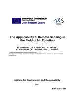
<i><b>Implementation steps and research methods </b></i>(Fig. 2)

<i>Geometric correction: </i>

Before analysis and interpretation, satellite images must be corrected geometrically
to limit position errors and terrain differences, which makes it easier to analyse and detect
changes. In addition, geometric corrections are also carried out to eliminate distortions
during photography and to return images to standard coordinates so that they can be
integrated with other data sources. To perform the geometric correction, the authors select
ground control points (GCPs). The coordinate parameters are included in the least-squares
regression analysis to determine the coefficients of the conversion equation between
images and map coordinates. After the conversion equation, the sample redistribution

“Clean day”
satellite image
“Polluted day”
satellite image
Geometric
correction
Radiation
correction

AOD calculate

Modified
algorithms

Earth station
measurements of PM10

concentration
Statistical analysis of PM10

concentration for each
image channel
Correlate calculations and
choose the best regression

function
Establish a PM10

concentration map
Remote sensing

methods

Statistical methods

<b>Fig. 2. Implementation steps and research methods </b>[8].

<b>Fig. 2. Implementation steps and research methods </b>[8].
<i><b>Geometric correction</b></i>

Before analysis and interpretation, satellite images

must be corrected geometrically to limit position errors
and terrain differences, which makes it easier to analyse
and detect changes. In addition, geometric corrections are
also carried out to eliminate distortions during photography
and to return images to standard coordinates so that they
can be integrated with other data sources. To perform the
geometric correction, the authors select ground control
points (GCPs). The coordinate parameters are included
in the least-squares regression analysis to determine the
coefficients of the conversion equation between images and
map coordinates. After the conversion equation, the sample
redistribution process is performed to determine the pixel
values included in the corrected image. The interpolation
methods that are applied in the re-division process are
interpolation and tertiary interpolation. In order to retain
the spatial and radiation quality of the image, the nearest
neighbour interpolation method is used over the whole
course of image processing.

<i><b>Radiation correction </b></i>[9-13]

Conversion to radiation values: this study uses remote
sensing images from Landsat 5 TM (used as “clean day”
images) and Landsat 8 (for the time of observation).

For the Landsat 5 TM:

L_λ= A x (DN - Q_min) + B (2)

where L_λ is the radiation value on the satellite (Wm-2_μm-1_),

Q_minis the minimum quantitative reflection value on the
pixel (Q_min=1), B is the minimum reflectance value, DN is
the reflection value per pixel, and A is the value calculated
by the following equation:

max min
max min

(

)

(

)

<i>L</i>

<i>L</i>

<i>A</i>

<i>Q</i>

<i>Q</i>

−

=

−

(3)

with L_max and L_minare the largest and smallest reflected
values, respectively, and Q_max and Q_min are the largest (255)
and smallest (1) quantised reflection values on the pixel
cell, respectively.

For the Landsat 8 OLI:

L_λ= M_Lx DN + A_L (4)

where M_L and A_L values are radiation multipliers and
additions calculated for each channel, respectively.

The values L_max and L_min, Q_max and Q_min, and M_L and A_L
are taken from an MTL file attached in the remote sensing
image file when downloaded.

Conversion to reflection values: for the Landsat 5 TM:
2

cos

<i>p</i>

<i>s</i>

<i>L d</i>

<i>ESUN</i>

λλ

π

ρ

θ

×

×

=

×

(5)

where <i>ρ_p</i> is the reflection value on the satellite corresponding
with wavelength λ, L_λ is the radiation value on the satellite
with unit Wm-2_.μm-1_{, ESUN}

λ is the average lighting of the
upper atmosphere from the Sun (Wm-2_.Μm-1_{), θ}

s is the angle
of the sun’s peak and the complementary angle of the Sun’s
elevation (θ_s = radians (90o_{- the angle of the Sun)) and}<i>_d</i>_is
the distance between Earth and Sun in astronomical units
and calculated using Smith’s equation (Eq. 6):

<i>d</i> = (1 - 0.01672 * cos(radians(0.9856 * (Julian Day - 4)))) (6)
with the Landsat 8 OLI, the reflectance value is calculated
as the surface reflectance value with Eq. 7:

(7)
with T_v and T_z being a function of transmitting atmospheric
radiation from the Earth’s surface to the receiver and from
<i>Geometric correction: </i>

Before analysis and interpretation, satellite images must be corrected geometrically
to limit position errors and terrain differences, which makes it easier to analyse and detect
changes. In addition, geometric corrections are also carried out to eliminate distortions
during photography and to return images to standard coordinates so that they can be
integrated with other data sources. To perform the geometric correction, the authors select
ground control points (GCPs). The coordinate parameters are included in the least-squares
regression analysis to determine the coefficients of the conversion equation between

images and map coordinates. After the conversion equation, the sample redistribution

“Clean day”
satellite image
“Polluted day”
satellite image
Geometric
correction
Radiation
correction

AOD calculate
Modified
algorithms

Earth station
measurements of PM10

concentration
Statistical analysis of PM10

concentration for each
image channel
Correlate calculations and
choose the best regression

function
Establish a PM10

concentration map

Remote sensing

methods

Statistical methods

<b>Fig. 2. Implementation steps and research methods </b>[8].
<i>Geometric correction: </i>

Before analysis and interpretation, satellite images must be corrected geometrically
to limit position errors and terrain differences, which makes it easier to analyse and detect
changes. In addition, geometric corrections are also carried out to eliminate distortions
during photography and to return images to standard coordinates so that they can be
integrated with other data sources. To perform the geometric correction, the authors select
ground control points (GCPs). The coordinate parameters are included in the least-squares
regression analysis to determine the coefficients of the conversion equation between
images and map coordinates. After the conversion equation, the sample redistribution

“Clean day”
satellite image
“Polluted day”
satellite image
Geometric
correction
Radiation
correction

AOD calculate
Modified
algorithms

Earth station
measurements of PM10

concentration
Statistical analysis of PM10

concentration for each
image channel
Correlate calculations and
choose the best regression

function
Establish a PM10

concentration map
Remote sensing

methods

Statistical methods

<b>Fig. 2. Implementation steps and research methods </b>[8].

<i>Geometric correction: </i>

Before analysis and interpretation, satellite images must be corrected geometrically
to limit position errors and terrain differences, which makes it easier to analyse and detect
changes. In addition, geometric corrections are also carried out to eliminate distortions
during photography and to return images to standard coordinates so that they can be

integrated with other data sources. To perform the geometric correction, the authors select
ground control points (GCPs). The coordinate parameters are included in the least-squares
regression analysis to determine the coefficients of the conversion equation between
images and map coordinates. After the conversion equation, the sample redistribution

“Clean day”
satellite image
“Polluted day”
satellite image
Geometric
correction
Radiation
correction

AOD calculate
Modified
algorithms

Earth station
measurements of PM10

concentration
Statistical analysis of PM10

concentration for each
image channel
Correlate calculations and
choose the best regression

function

Establish a PM10

concentration map
Remote sensing

methods

Statistical methods

</div>
<span class='text_page_counter'>(4)</span><div class='page_container' data-page=4>

<i><b>EnvironmEntal SciEncES </b></i>|<i> Ecology</i>

<b>Vietnam Journal of Science,</b>

<b>Technology and Engineering</b>

90

December 2020 • Volume 62 Number 4

the Sun to the Earth, respectively, ESUN_λ is the average
lighting of the upper atmosphere from the Sun (Wm-2_Μm-1_),
E_down is the spectral radiation going to the object’s terrain
surface, <i>d</i> is the distance between the Earth and the Sun and
L_P is the line radiation calculated by the following Eq. 8:

(8)
Based on the DOS method, the determination of T_V, T_Z,
and E_down parameters which divided into many different
methods (DOS1, DOS2, DOS3, DOS4) having different
accuracy. In this study, the authors use DOS1, in which
the parameters were determined by Moran and his team as
T_V=1; T_Z=1; and E_down = 0. At this time Eq. 7 will become:

(9)

with L_pis calculated by Eq. 10:

(10)
<i><b>The algorithm calculates AOD</b></i>

<i>“Blur” effect: </i>after radiation correction, the authors have

an image showing the reflection value of the objects. Based
on the results of the reflection, the authors proceed to extract
AOD by the method of N. Sifakis and P-Y. Deschamps
(1992) [14]. The team used 2 remote sensing images,
one in completely clean air (used as a “reference image”)
and the other in polluted air for the survey. According to
the previous study, surface radiation is a space-dependent
variable and is not time based, so using differential textural
analysis (DTA), the team extracted the approximate value
of AOD [14].

In the visible light spectrum of electromagnetic waves, the scattering of shortwave
radiation is mostly caused by particulate matter in the atmosphere that causes a decrease
in the contrast and distortion of the spectral feedback pattern in the remote sensing image
(Fig. 3). This is called the "blurring" effect, which can be estimated using the optical
depth (OD) derived from the basic equation of the apparent reflection from a satellite. For
research objects in a large space (with a radius within 1 km) and homogeneity between
different objects, the authors have the equation of "clear" reflection as follows:

= () ( ) + (11)

where ρ*_{, ρ}_,_{and ρ}_{a are "clear" reflections in satellites, surface reflections, and atmospheric}
reflections, respectively. S is the spherical reflectance of the atmosphere defined as the
ratio of scattering to total attenuation of radiation, θs and θv are the Sun's zenith angles
and their zenith angles, respectively. T(θs) is the total transmission function on the

“downlink”, it can be analysed as the sum of tdir(θs) and tdiff(θs) including direct and
diffusion transfer functions. T(θv) is the total transmission function on the uplink and it
can be analysed as the sum of tdir(θv) and tdiff(θv) including direct and diffusion transfer
functions. According to Eq. 11, the authors obtain information about optical thickness as a

function of ρa with ρ≈0. However, for research areas having small diameters (<100 m),
the authors need to consider the proximity effect and Eq. 1 needs to consider the average

reflection of the surrounding objects (ρe). Then Eq. 11 will become:
= ( ) ( )

+

( )( )

+ (12)

According to the authors, standard deviation is an indicator of similar contrast as
seen on satellite images. So N. Sifakis and P-Y. Deschamps (1992) [14] have given the

correlation equation between the standard deviation of the "clear" (σ(ρ*_{)) reflectance and}
the standard deviation of the true reflectance (σ(ρ)) based on Eq. 12. The authors took a
random set of adjacent pixel cells and found that the change of (σ(ρ*_{)) is only affected by}

the standard deviation of the actual reflection at the surface (σ(ρ)). Therefore, the authors

obtained the following correlation equation:
( ) = ( ) ( ) ( )

(13)

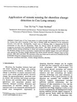
<b>Fig. 3. Different components of total radiation transmitted up and down </b>[14]<b>.</b>

In the visible light spectrum of electromagnetic waves, the scattering of shortwave
radiation is mostly caused by particulate matter in the atmosphere that causes a decrease
in the contrast and distortion of the spectral feedback pattern in the remote sensing image
(Fig. 3). This is called the "blurring" effect, which can be estimated using the optical
depth (OD) derived from the basic equation of the apparent reflection from a satellite. For
research objects in a large space (with a radius within 1 km) and homogeneity between
different objects, the authors have the equation of "clear" reflection as follows:

= () ( ) + (11)

where ρ*_{, ρ}_,_{and ρ}_{a are "clear" reflections in satellites, surface reflections, and atmospheric}
reflections, respectively. S is the spherical reflectance of the atmosphere defined as the
ratio of scattering to total attenuation of radiation, θs and θv are the Sun's zenith angles
and their zenith angles, respectively. T(θs) is the total transmission function on the

“downlink”, it can be analysed as the sum of tdir(θs) and tdiff(θs) including direct and
diffusion transfer functions. T(θv) is the total transmission function on the uplink and it
can be analysed as the sum of tdir(θv) and tdiff(θv) including direct and diffusion transfer
functions. According to Eq. 11, the authors obtain information about optical thickness as a

function of ρa with ρ≈0. However, for research areas having small diameters (<100 m),

the authors need to consider the proximity effect and Eq. 1 needs to consider the average

reflection of the surrounding objects (ρe). Then Eq. 11 will become:
= ( ) ( )

+

( )( )

+ (12)

According to the authors, standard deviation is an indicator of similar contrast as
seen on satellite images. So N. Sifakis and P-Y. Deschamps (1992) [14] have given the

correlation equation between the standard deviation of the "clear" (σ(ρ*_{)) reflectance and}
the standard deviation of the true reflectance (σ(ρ)) based on Eq. 12. The authors took a
random set of adjacent pixel cells and found that the change of (σ(ρ*_{)) is only affected by}

the standard deviation of the actual reflection at the surface (σ(ρ)). Therefore, the authors

obtained the following correlation equation:
( ) = ( ) ( ) ( )

(13)

<b>Fig. 3. Different components of total radiation transmitted up and down Fig. 3. Different components of total radiation transmitted up </b>[14]<b>.</b>

<b>and down </b>[14].

In the visible light spectrum of electromagnetic waves,

the scattering of shortwave radiation is mostly caused by
particulate matter in the atmosphere that causes a decrease
in the contrast and distortion of the spectral feedback pattern
in the remote sensing image (Fig. 3). This is called the
“blurring” effect, which can be estimated using the optical

depth (OD) derived from the basic equation of the apparent
reflection from a satellite. For research objects in a large
space (with a radius within 1 km) and homogeneity between
different objects, the authors have the equation of “clear”
reflection as follows:

In the visible light spectrum of electromagnetic waves, the scattering of shortwave
radiation is mostly caused by particulate matter in the atmosphere that causes a decrease
in the contrast and distortion of the spectral feedback pattern in the remote sensing image
(Fig. 3). This is called the "blurring" effect, which can be estimated using the optical
depth (OD) derived from the basic equation of the apparent reflection from a satellite. For
research objects in a large space (with a radius within 1 km) and homogeneity between
different objects, the authors have the equation of "clear" reflection as follows:

= ( ) ( )

+ (11)
where ρ*_{, ρ}_,_{and ρ}_{a are "clear" reflections in satellites, surface reflections, and atmospheric}
reflections, respectively. S is the spherical reflectance of the atmosphere defined as the
ratio of scattering to total attenuation of radiation, θs and θv are the Sun's zenith angles
and their zenith angles, respectively. T(θs) is the total transmission function on the

“downlink”, it can be analysed as the sum of tdir(θs) and tdiff(θs) including direct and
diffusion transfer functions. T(θv) is the total transmission function on the uplink and it

can be analysed as the sum of tdir(θv) and tdiff(θv) including direct and diffusion transfer
functions. According to Eq. 11, the authors obtain information about optical thickness as a

function of ρa with ρ≈0. However, for research areas having small diameters (<100 m),
the authors need to consider the proximity effect and Eq. 1 needs to consider the average

reflection of the surrounding objects (ρe). Then Eq. 11 will become:
= ( ) ( )

+

( ) ( )

+ (12)

According to the authors, standard deviation is an indicator of similar contrast as
seen on satellite images. So N. Sifakis and P-Y. Deschamps (1992) [14] have given the

correlation equation between the standard deviation of the "clear" (σ(ρ*_{)) reflectance and}
the standard deviation of the true reflectance (σ(ρ)) based on Eq. 12. The authors took a
random set of adjacent pixel cells and found that the change of (σ(ρ*_{)) is only affected by}

the standard deviation of the actual reflection at the surface (σ(ρ)). Therefore, the authors

obtained the following correlation equation:
( ) = ( ) ( ) ( )

(13)

<b>Fig. 3. Different components of total radiation transmitted up and down </b>[14]<b>.</b>

(11)

where ρ*_{, ρ, and ρ}

a are “clear” reflections in satellites, surface
reflections, and atmospheric reflections, respectively. S
is the spherical reflectance of the atmosphere defined as
the ratio of scattering to total attenuation of radiation, θs
and θv are the Sun’s zenith angles and their zenith angles,
respectively. T(θ_s) is the total transmission function on the
“downlink”, it can be analysed as the sum of t_dir(θ_s) and
t_diff(θ_s) including direct and diffusion transfer functions.
T(θ_v) is the total transmission function on the uplink and it
can be analysed as the sum of t_dir(θ_v) and t_diff(θ_v) including
direct and diffusion transfer functions. According to Eq. 11,
the authors obtain information about optical thickness as a
function of ρ_a with ρ≈0. However, for research areas having
small diameters (<100 m), the authors need to consider the
proximity effect and Eq. 1 needs to consider the average
reflection of the surrounding objects (ρ_e). Then Eq. 11 will
become:

In the visible light spectrum of electromagnetic waves, the scattering of shortwave
radiation is mostly caused by particulate matter in the atmosphere that causes a decrease
in the contrast and distortion of the spectral feedback pattern in the remote sensing image
(Fig. 3). This is called the "blurring" effect, which can be estimated using the optical
depth (OD) derived from the basic equation of the apparent reflection from a satellite. For
research objects in a large space (with a radius within 1 km) and homogeneity between
different objects, the authors have the equation of "clear" reflection as follows:

= () ( ) + (11)

where ρ*_{, ρ}_,_{and ρ}_{a are "clear" reflections in satellites, surface reflections, and atmospheric}
reflections, respectively. S is the spherical reflectance of the atmosphere defined as the
ratio of scattering to total attenuation of radiation, θs and θv are the Sun's zenith angles
and their zenith angles, respectively. T(θs) is the total transmission function on the

“downlink”, it can be analysed as the sum of tdir(θs) and tdiff(θs) including direct and
diffusion transfer functions. T(θv) is the total transmission function on the uplink and it
can be analysed as the sum of tdir(θv) and tdiff(θv) including direct and diffusion transfer
functions. According to Eq. 11, the authors obtain information about optical thickness as a

function of ρa with ρ≈0. However, for research areas having small diameters (<100 m),
the authors need to consider the proximity effect and Eq. 1 needs to consider the average

reflection of the surrounding objects (ρe). Then Eq. 11 will become:
= ( ) ( )

+

( ) ( )

+ (12)

According to the authors, standard deviation is an indicator of similar contrast as
seen on satellite images. So N. Sifakis and P-Y. Deschamps (1992) [14] have given the

correlation equation between the standard deviation of the "clear" (σ(ρ*_{)) reflectance and}
the standard deviation of the true reflectance (σ(ρ)) based on Eq. 12. The authors took a

random set of adjacent pixel cells and found that the change of (σ(ρ*_{)) is only affected by}

the standard deviation of the actual reflection at the surface (σ(ρ)). Therefore, the authors

obtained the following correlation equation:
( ) = ( ) ( ) ( )

(13)

<b>Fig. 3. Different components of total radiation transmitted up and down </b>[14]<b>.</b>

(12)
According to the authors, standard deviation is an
indicator of similar contrast as seen on satellite images. So
N. Sifakis and P-Y. Deschamps (1992) [14] have given the
correlation equation between the standard deviation of the
“clear” (σ(ρ*_{)) reflectance and the standard deviation of the}
true reflectance (σ(ρ)) based on Eq. 12. The authors took a
random set of adjacent pixel cells and found that the change
of (σ(ρ*_{)) is only affected by the standard deviation of the}
actual reflection at the surface (σ(ρ)). Therefore, the authors
obtained the following correlation equation:

In the visible light spectrum of electromagnetic waves, the scattering of shortwave
radiation is mostly caused by particulate matter in the atmosphere that causes a decrease
in the contrast and distortion of the spectral feedback pattern in the remote sensing image
(Fig. 3). This is called the "blurring" effect, which can be estimated using the optical
depth (OD) derived from the basic equation of the apparent reflection from a satellite. For
research objects in a large space (with a radius within 1 km) and homogeneity between
different objects, the authors have the equation of "clear" reflection as follows:

= () ( ) + (11)

where ρ*_{, ρ}_,_{and ρ}_{a are "clear" reflections in satellites, surface reflections, and atmospheric}
reflections, respectively. S is the spherical reflectance of the atmosphere defined as the
ratio of scattering to total attenuation of radiation, θs and θv are the Sun's zenith angles
and their zenith angles, respectively. T(θs) is the total transmission function on the

“downlink”, it can be analysed as the sum of tdir(θs) and tdiff(θs) including direct and
diffusion transfer functions. T(θv) is the total transmission function on the uplink and it
can be analysed as the sum of tdir(θv) and tdiff(θv) including direct and diffusion transfer
functions. According to Eq. 11, the authors obtain information about optical thickness as a

function of ρa with ρ≈0. However, for research areas having small diameters (<100 m),
the authors need to consider the proximity effect and Eq. 1 needs to consider the average

reflection of the surrounding objects (ρe). Then Eq. 11 will become:
= ( ) ( )

+

( )( )

+ (12)

According to the authors, standard deviation is an indicator of similar contrast as
seen on satellite images. So N. Sifakis and P-Y. Deschamps (1992) [14] have given the

correlation equation between the standard deviation of the "clear" (σ(ρ*_{)) reflectance and}
the standard deviation of the true reflectance (σ(ρ)) based on Eq. 12. The authors took a

random set of adjacent pixel cells and found that the change of (σ(ρ*_{)) is only affected by}

the standard deviation of the actual reflection at the surface (σ(ρ)). Therefore, the authors

obtained the following correlation equation:
( ) = ( ) ( ) ( )

(13)

<b>Fig. 3. Different components of total radiation transmitted up and down </b>[14]<b>.</b>

(13)
Appling the Lambert - Bouguer transmission law to the
transmission function t_dir(θ_v), the authors calibrate it to the

angle θAppling the Lambert - Bouguer transmission law to the transmission function _v and the following equation is found:
tdir(θv), the authors calibrate it to the angle θv and the following equation is found:

( ) = ( ) ( ) ( ) (14)
According to Eq. 14, <i>-τ/cos(θv) </i>can be seen as AOD, which is calibrated to the
Sun's angle.

<i>Pixel: </i>as mentioned above, following by the method of N. Sifakis and P-Y.
Deschamps (1992) [14], the authors divide the study area into random pixel cells to
calculate the reflectance standard deviation of the area.

<i>AOD calculation:</i>based on Eq. 14, the authors can calculate the standard deviation
of the clean day and pollution day. Then, they take the equation for the clean day and
divide by the pollution day, which yields the following equation:

( )

( ) = exp(( ( ) ( ( )) (15)

Landsat-8/OLI has zero viewing angles or zenith views at the center of the image.
The maximum value of the view at the edges of the frame is 7.4960 calculated from the
height of Landsat 8 satellite (703 km) and the width of 185 km. Hence the viewing angle
range is from 0-7.4960 for any satellite image. For the Landsat 5 TM of the clean day
image, the authors calculated the same zenith view from which the authors see that the
clean day image angle ranged from 0-7.3950. Because the angle of view is small, the

authors can assume that cos (θv1) ≈ cos (θv2) ≈ 1 and an error of ≈ 0.4%:

( )

( ) = exp (- - ) (16)

with and is the atmospheric depth in the clean day and the pollution day,
respectively. Based on Eq. 16, the authors calculate the AOD difference between the
clean day and the pollution day as:

= - = ln[ ( )

( )] (17)

In Eq. 17, the AOD is equal to the difference of optical depth in the clean and
polluted images. However, for "clean days", the atmosphere is assumed to be completely
"transparent" so it is possible to indicate that the optical depth on a clean day is

approximately zero (τ1 ≈ 0). So, from Eq. 17, the authors obtain the following equation:

= = ln[ (₍ )₎] (18)

The optical depth difference of the clean day and pollution day is also the optical
(14)

According to Eq. 14, <i>-τ/cos(θ_v) </i>can be seen as AOD,
which is calibrated to the Sun’s angle.

</div>
<span class='text_page_counter'>(5)</span><div class='page_container' data-page=5>

<i><b>EnvironmEntal SciEncES </b></i>|<i> Ecology</i>

<b>Vietnam Journal of Science,</b>

<b>Technology and Engineering</b>

91

December 2020 • Volume 62 Number 4

<i>AOD calculation:</i> based on Eq. 14, the authors can
calculate the standard deviation of the clean day and
pollution day. Then, they take the equation for the clean day
and divide by the pollution day, which yields the following
equation:

Appling the Lambert - Bouguer transmission law to the transmission function
tdir(θv), the authors calibrate it to the angle θv and the following equation is found:

( ) = ( ) ( ) ( ) (14)
According to Eq. 14, <i>-τ/cos(θv) </i>can be seen as AOD, which is calibrated to the
Sun's angle.

<i>Pixel: </i>as mentioned above, following by the method of N. Sifakis and P-Y.
Deschamps (1992) [14], the authors divide the study area into random pixel cells to

calculate the reflectance standard deviation of the area.

<i>AOD calculation:</i>based on Eq. 14, the authors can calculate the standard deviation
of the clean day and pollution day. Then, they take the equation for the clean day and
divide by the pollution day, which yields the following equation:

( )

( ) = exp(( ( ) ( ( )) (15)

Landsat-8/OLI has zero viewing angles or zenith views at the center of the image.
The maximum value of the view at the edges of the frame is 7.4960 calculated from the
height of Landsat 8 satellite (703 km) and the width of 185 km. Hence the viewing angle
range is from 0-7.4960 for any satellite image. For the Landsat 5 TM of the clean day
image, the authors calculated the same zenith view from which the authors see that the
clean day image angle ranged from 0-7.3950. Because the angle of view is small, the

authors can assume that cos (θv1) ≈ cos (θv2) ≈ 1 and an error of ≈ 0.4%:

( )

( ) = exp (- - ) (16)

with and is the atmospheric depth in the clean day and the pollution day,
respectively. Based on Eq. 16, the authors calculate the AOD difference between the
clean day and the pollution day as:

= - = ln[ ( )

( )] (17)

In Eq. 17, the AOD is equal to the difference of optical depth in the clean and
polluted images. However, for "clean days", the atmosphere is assumed to be completely
"transparent" so it is possible to indicate that the optical depth on a clean day is

approximately zero (τ1 ≈ 0). So, from Eq. 17, the authors obtain the following equation:

= = ln[ (₍ )₎] (18)

The optical depth difference of the clean day and pollution day is also the optical
depth of the pollution day and is determined by Eq. 18 [14-16].

<b>Results </b>

<i><b>Correlation and regression analysis between real AOD and PM</b><b>10</b></i>

(15)
Landsat-8/OLI has zero viewing angles or zenith views
at the center of the image. The maximum value of the
view at the edges of the frame is 7.4960 calculated from
the height of Landsat 8 satellite (703 km) and the width of
185 km. Hence the viewing angle range is from 0-7.4960
for any satellite image. For the Landsat 5 TM of the clean
day image, the authors calculated the same zenith view
from which the authors see that the clean day image angle
ranged from 0-7.3950. Because the angle of view is small,
the authors can assume that cos (θ_v1) ≈ cos (θ_v2) ≈ 1 and an
error of ≈ 0.4%:

Appling the Lambert - Bouguer transmission law to the transmission function

tdir(θv), the authors calibrate it to the angle θv and the following equation is found:

( ) = ( ) ( ) ( )

(14)

According to Eq. 14, <i>-τ/cos(θv) </i>can be seen as AOD, which is calibrated to the
Sun's angle.

<i>Pixel: </i>as mentioned above, following by the method of N. Sifakis and P-Y.
Deschamps (1992) [14], the authors divide the study area into random pixel cells to
calculate the reflectance standard deviation of the area.

<i>AOD calculation:</i>based on Eq. 14, the authors can calculate the standard deviation
of the clean day and pollution day. Then, they take the equation for the clean day and
divide by the pollution day, which yields the following equation:

( )

( ) = exp(( ( ) ( ( )) (15)

Landsat-8/OLI has zero viewing angles or zenith views at the center of the image.
The maximum value of the view at the edges of the frame is 7.4960 calculated from the
height of Landsat 8 satellite (703 km) and the width of 185 km. Hence the viewing angle
range is from 0-7.4960 for any satellite image. For the Landsat 5 TM of the clean day
image, the authors calculated the same zenith view from which the authors see that the
clean day image angle ranged from 0-7.3950. Because the angle of view is small, the

authors can assume that cos (θv1) ≈ cos (θv2) ≈ 1 and an error of ≈ 0.4%:

( )

( ) = exp (- - ) (16)

with and is the atmospheric depth in the clean day and the pollution day,
respectively. Based on Eq. 16, the authors calculate the AOD difference between the
clean day and the pollution day as:

= - = ln[ (₍ )₎] (17)

In Eq. 17, the AOD is equal to the difference of optical depth in the clean and
polluted images. However, for "clean days", the atmosphere is assumed to be completely
"transparent" so it is possible to indicate that the optical depth on a clean day is

approximately zero (τ1 ≈ 0). So, from Eq. 17, the authors obtain the following equation:

= = ln[ (₍ )₎] (18)

The optical depth difference of the clean day and pollution day is also the optical
depth of the pollution day and is determined by Eq. 18 [14-16].

<b>Results </b>

<i><b>Correlation and regression analysis between real AOD and PM</b><b>10</b></i>

(16)
with

Appling the Lambert - Bouguer transmission law to the transmission function
tdir(θv), the authors calibrate it to the angle θv and the following equation is found:

( ) = ( ) ( ) ( ) (14)
According to Eq. 14, <i>-τ/cos(θv) </i>can be seen as AOD, which is calibrated to the
Sun's angle.

<i>Pixel: </i>as mentioned above, following by the method of N. Sifakis and P-Y.
Deschamps (1992) [14], the authors divide the study area into random pixel cells to
calculate the reflectance standard deviation of the area.

<i>AOD calculation:</i>based on Eq. 14, the authors can calculate the standard deviation
of the clean day and pollution day. Then, they take the equation for the clean day and
divide by the pollution day, which yields the following equation:

( )

( ) = exp(( ( ) ( ( )) (15)

Landsat-8/OLI has zero viewing angles or zenith views at the center of the image.
The maximum value of the view at the edges of the frame is 7.4960 calculated from the
height of Landsat 8 satellite (703 km) and the width of 185 km. Hence the viewing angle
range is from 0-7.4960 for any satellite image. For the Landsat 5 TM of the clean day
image, the authors calculated the same zenith view from which the authors see that the
clean day image angle ranged from 0-7.3950. Because the angle of view is small, the

authors can assume that cos (θv1) ≈ cos (θv2) ≈ 1 and an error of ≈ 0.4%:

( )

( ) = exp (- - ) (16)

with and is the atmospheric depth in the clean day and the pollution day,
respectively. Based on Eq. 16, the authors calculate the AOD difference between the
clean day and the pollution day as:

= - = ln[ ( )

( )] (17)

In Eq. 17, the AOD is equal to the difference of optical depth in the clean and
polluted images. However, for "clean days", the atmosphere is assumed to be completely
"transparent" so it is possible to indicate that the optical depth on a clean day is

approximately zero (τ1 ≈ 0). So, from Eq. 17, the authors obtain the following equation:

= = ln[ (₍ )₎] (18)

The optical depth difference of the clean day and pollution day is also the optical
depth of the pollution day and is determined by Eq. 18 [14-16].

<b>Results </b>

<i><b>Correlation and regression analysis between real AOD and PM</b><b>10</b></i>

and

Appling the Lambert - Bouguer transmission law to the transmission function
tdir(θv), the authors calibrate it to the angle θv and the following equation is found:

( ) = ( ) ( ) ( ) (14)
According to Eq. 14, <i>-τ/cos(θv) </i>can be seen as AOD, which is calibrated to the

Sun's angle.

<i>Pixel: </i>as mentioned above, following by the method of N. Sifakis and P-Y.
Deschamps (1992) [14], the authors divide the study area into random pixel cells to
calculate the reflectance standard deviation of the area.

<i>AOD calculation:</i>based on Eq. 14, the authors can calculate the standard deviation
of the clean day and pollution day. Then, they take the equation for the clean day and
divide by the pollution day, which yields the following equation:

( )

( ) = exp(( ( ) ( ( )) (15)

Landsat-8/OLI has zero viewing angles or zenith views at the center of the image.
The maximum value of the view at the edges of the frame is 7.4960 calculated from the
height of Landsat 8 satellite (703 km) and the width of 185 km. Hence the viewing angle
range is from 0-7.4960 for any satellite image. For the Landsat 5 TM of the clean day
image, the authors calculated the same zenith view from which the authors see that the
clean day image angle ranged from 0-7.3950. Because the angle of view is small, the

authors can assume that cos (θv1) ≈ cos (θv2) ≈ 1 and an error of ≈ 0.4%:

( )

( ) = exp (- - ) (16)

with and is the atmospheric depth in the clean day and the pollution day,
respectively. Based on Eq. 16, the authors calculate the AOD difference between the
clean day and the pollution day as:

= - = ln[ (₍ )₎] (17)

In Eq. 17, the AOD is equal to the difference of optical depth in the clean and
polluted images. However, for "clean days", the atmosphere is assumed to be completely
"transparent" so it is possible to indicate that the optical depth on a clean day is

approximately zero (τ1 ≈ 0). So, from Eq. 17, the authors obtain the following equation:
= = ln[ ( )

( )] (18)

The optical depth difference of the clean day and pollution day is also the optical
depth of the pollution day and is determined by Eq. 18 [14-16].

<b>Results </b>

<i><b>Correlation and regression analysis between real AOD and PM</b><b>10</b></i>

is the atmospheric depth in the clean day and
the pollution day, respectively. Based on Eq. 16, the authors
calculate the AOD difference between the clean day and the
pollution day as:

Appling the Lambert - Bouguer transmission law to the transmission function
tdir(θv), the authors calibrate it to the angle θv and the following equation is found:

( ) = ( ) ( ) ( ) (14)
According to Eq. 14, <i>-τ/cos(θv) </i>can be seen as AOD, which is calibrated to the
Sun's angle.

<i>Pixel: </i>as mentioned above, following by the method of N. Sifakis and P-Y.
Deschamps (1992) [14], the authors divide the study area into random pixel cells to
calculate the reflectance standard deviation of the area.

<i>AOD calculation:</i>based on Eq. 14, the authors can calculate the standard deviation
of the clean day and pollution day. Then, they take the equation for the clean day and
divide by the pollution day, which yields the following equation:

( )

( ) = exp(( ( ) ( ( )) (15)

Landsat-8/OLI has zero viewing angles or zenith views at the center of the image.
The maximum value of the view at the edges of the frame is 7.4960 calculated from the
height of Landsat 8 satellite (703 km) and the width of 185 km. Hence the viewing angle
range is from 0-7.4960 for any satellite image. For the Landsat 5 TM of the clean day
image, the authors calculated the same zenith view from which the authors see that the
clean day image angle ranged from 0-7.3950. Because the angle of view is small, the

authors can assume that cos (θv1) ≈ cos (θv2) ≈ 1 and an error of ≈ 0.4%:

( )

( ) = exp (- - ) (16)

with and is the atmospheric depth in the clean day and the pollution day,
respectively. Based on Eq. 16, the authors calculate the AOD difference between the
clean day and the pollution day as:

= - = ln[ (₍ )₎] (17)

In Eq. 17, the AOD is equal to the difference of optical depth in the clean and
polluted images. However, for "clean days", the atmosphere is assumed to be completely
"transparent" so it is possible to indicate that the optical depth on a clean day is

approximately zero (τ1 ≈ 0). So, from Eq. 17, the authors obtain the following equation:
= = ln[ ( )

( )] (18)

The optical depth difference of the clean day and pollution day is also the optical
depth of the pollution day and is determined by Eq. 18 [14-16].

<b>Results </b>

<i><b>Correlation and regression analysis between real AOD and PM</b><b>10</b></i>

(17)
In Eq. 17, the AOD is equal to the difference of optical
depth in the clean and polluted images. However, for
“clean days”, the atmosphere is assumed to be completely
“transparent” so it is possible to indicate that the optical
depth on a clean day is approximately zero (τ₁ ≈ 0). So, from
Eq. 17, the authors obtain the following equation:

Appling the Lambert - Bouguer transmission law to the transmission function
tdir(θv), the authors calibrate it to the angle θv and the following equation is found:

( ) = ( ) ( ) ( )

(14)

According to Eq. 14, <i>-τ/cos(θv) </i>can be seen as AOD, which is calibrated to the
Sun's angle.

<i>Pixel: </i>as mentioned above, following by the method of N. Sifakis and P-Y.
Deschamps (1992) [14], the authors divide the study area into random pixel cells to
calculate the reflectance standard deviation of the area.

<i>AOD calculation:</i>based on Eq. 14, the authors can calculate the standard deviation
of the clean day and pollution day. Then, they take the equation for the clean day and
divide by the pollution day, which yields the following equation:

( )

( ) = exp(( ( ) ( ( )) (15)

Landsat-8/OLI has zero viewing angles or zenith views at the center of the image.
The maximum value of the view at the edges of the frame is 7.4960 calculated from the
height of Landsat 8 satellite (703 km) and the width of 185 km. Hence the viewing angle
range is from 0-7.4960 for any satellite image. For the Landsat 5 TM of the clean day
image, the authors calculated the same zenith view from which the authors see that the
clean day image angle ranged from 0-7.3950. Because the angle of view is small, the

authors can assume that cos (θv1) ≈ cos (θv2) ≈ 1 and an error of ≈ 0.4%:

( )

( ) = exp (- - ) (16)

with and is the atmospheric depth in the clean day and the pollution day,
respectively. Based on Eq. 16, the authors calculate the AOD difference between the
clean day and the pollution day as:

= - = ln[ (₍ )₎] (17)

In Eq. 17, the AOD is equal to the difference of optical depth in the clean and
polluted images. However, for "clean days", the atmosphere is assumed to be completely
"transparent" so it is possible to indicate that the optical depth on a clean day is

approximately zero (τ1 ≈ 0). So, from Eq. 17, the authors obtain the following equation:

= = ln[ (₍ )₎] (18)

The optical depth difference of the clean day and pollution day is also the optical
depth of the pollution day and is determined by Eq. 18 [14-16].

<b>Results </b>

<i><b>Correlation and regression analysis between real AOD and PM</b><b>10</b></i>

(18)
The optical depth difference of the clean day and
pollution day is also the optical depth of the pollution day
and is determined by Eq. 18 [14-16].

<b>Results</b>

<i><b>Correlation and regression analysis between real AOD </b></i>

<i><b>and PM</b><b>₁₀</b></i>

Like most of the other studies on AOD determination as
well as PM₁₀ concentration distribution by remote sensing,
this study conducted AOD surveys mainly on 4 spectral
channels: the blue spectrum channel (0.450-0.515 µm),
green spectrum channel (0.525-0.600 µm), red spectrum
(0.630-0.680 µm), and near-infrared channel (0.845-0.885
µm). Table 1 shows the results obtained when extracting
AOD from the 4 image channels.

<b>Table 1. AOD extract results from 4 channels Landsat image.</b>

<b>Stations</b> <b>PM10 concentration</b>
<b>(μg/m3₎</b>

<b>AOD in 28th_{Feb, 2017}</b>

<i><b>Blue</b></i> <i><b>Green</b></i> <i><b>Red</b></i> <i><b>Near-infrared </b></i>

Zoo 66.4 -1.08318 -2.59237 -1.09258 -1.75548
Binh Chanh 138.5 -3.06638 -2.13509 -4.91728 -2.47673
DOSTE 112 -1.20462 -2.30867 -1.60878 -1.7548
Hong Bang 74.7 -2.04362 -3.58543 -2.67132 -1.14265
Thong Nhat Hospital 87 -2.04362 -3.78751 -1.92392 -2.33622
Tan Son Hoa 96.4 -1.99765 -3.91204 -2.05347 -1.45789

District 2 65 Noise Noise Noise -2.67964

According to these results, the authors established scatter

plots with AOD extracted as an independent variable (x)
and the actual PM₁₀concentration as the dependent variable
(y). Then, a regression equations was found and the results
are given in Figs. 4-7.

<b>Fig. 4. The correlation between PM₁₀ and AOD in the blue </b>
<b>channel. (A) </b>linear regression;<b> (B) </b>non-linear regression.

<b>Fig. 5. The correlation between PM₁₀ and AOD in the green </b>
<b>channel. (A) </b>linear regression;<b> (B) </b>non-linear regression.

<b>Fig. 6. The correlation between PM10 and AOD in the red </b>

<b>channel. (A) </b>linear regression; <b>(B) </b>non-linear regression.

<b>Fig. 7. The correlation between PM10 and AOD in the </b>

</div>
<span class='text_page_counter'>(6)</span><div class='page_container' data-page=6>

<i><b>EnvironmEntal SciEncES </b></i>|<i> Ecology</i>

<b>Vietnam Journal of Science,</b>

<b>Technology and Engineering</b>

92

December 2020 • Volume 62 Number 4

Through the analysis of the results (Table 2), the authors
found that the non-linear regression equation of the blue
spectrum channel gives the best correlation results between
the two parameters (with R2_{=0.9489). Therefore, the authors}
use non-linear regression between AOD and PM₁₀ on the
green channel [17].

<i><b>Evaluation of the error between the actual measured </b></i>
<i><b>dust concentration and the calculated dust concentration </b></i>
(Table 3)

<b>Table 3. Assessment of the error between the actual measured </b>
<b>concentration and the simulated concentration.</b>

<b>Station</b> <b>Calculated PMconcentration 10 </b>

<b>(μg/m3₎</b>

<b>Measured PM10</b>

<b>concentration </b>

<b>(μg/m3₎</b>

<b>Absolute </b>
<b>error</b>

Zoo 66.4 41.9 24.5

Binh Chanh 138.5 124.1 14.4

DOSTE 112 102.2 9.8

Hong Bang 74.7 61.3 13.4

Thong Nhat Hospital 87 82.6 4.4

Tan Son Hoa 96.4 94.1 2.3

Error RMSE 13.5883

<i><b>Dust distribution map of Ho Chi Minh city area</b></i>
Hospital

Tan Son Hoa 96.4 94.1 2.3

Error RMSE 13.5883

<i><b>Dust distribution map of Ho Chi Minh city area </b></i>

The spatial concentration of the PM10 map was established in Ho Chi Minh city
(Fig. 8). The map shows the concentration of dust in the area at 10 am, which is the time
that vehicles and factories being operating. At this time, trucks are also allowed to run in
the downtown area.

It can be seen that the PM10 concentration is highest, at over 300 µg/m3, in districts
with high traffic density and a concentration of many industrial parks such as Binh
Chanh, Thu Duc, and district 9. Typically, in the area around the Thu Duc district, there
are up to 150 factories with large production scale and thousands of small factories.
Similarly, in the area around the Binh Chanh district, not only are there two large
industrial parks Ho Chi Minh city, the Vinh Loc and Le Minh Xuan industrial parks, there
are also many key roads such as the national highway 1A. High traffic volume also
contributes to the high amount of dust and smoke in the Binh Chanh district compared to
other areas.

In addition, Fig. 9 shows that PM10 concentration is distributed mainly in the

western areas of the Hoc Mon and Binh Chanh districts and then disperses to surrounding

<b>Fig. 8. Spatial concentration of PMFig. 8. Spatial concentration of PM10 in Ho Chi Minh city in February 28₁₀ in Ho Chi Minh city in th, 2017.</b>

<b>February 28th, 2017.</b>

The spatial concentration of the PM₁₀ map was

established in Ho Chi Minh city (Fig. 8). The map shows
the concentration of dust in the area at 10 am, which is the

time that vehicles and factories being operating. At this
time, trucks are also allowed to run in the downtown area.

It can be seen that the PM₁₀ concentration is highest, at
over 300 µg/m3_{, in districts with high traffic density and a}
concentration of many industrial parks such as Binh Chanh,
Thu Duc, and district 9. Typically, in the area around the
Thu Duc district, there are up to 150 factories with large
production scale and thousands of small factories. Similarly,
in the area around the Binh Chanh district, not only are there
two large industrial parks Ho Chi Minh city, the Vinh Loc
and Le Minh Xuan industrial parks, there are also many key
roads such as the national highway 1A. High traffic volume
also contributes to the high amount of dust and smoke in the
Binh Chanh district compared to other areas.

In addition, Fig. 9 shows that PM₁₀ concentration is
distributed mainly in the western areas of the Hoc Mon
and Binh Chanh districts and then disperses to surrounding

areas. It can be understood that the process of dispersing
suspended matter in the air is still influenced by the wind,
but the inner city has a large surface roughness due to many
high-rise buildings. So, a monsoon does not affect much in
the inner city, only a “whirlwind” does. The characteristic
of this wind is to blow along many directions under the
influence of the moving flow of vehicles as well as the
processes of heat emission from human activities.

In order to consider changes in PM₁₀ concentration over
time, the authors use the correlation equation obtained over
a number of years between 2009-2019. The years selected
for the analysis are selected according to the following
criteria: photos are available in February each year; selected
images with little cloud cover; in the period of 10 years
between 2009-2019.

Based on the above criteria, the authors choose 4 years
including February 11th_{, 2010, February 9}th_{, 2015, February}
28th_{, 2016, and February 17}th_{, 2018. The authors obtained}
the research results shown in Fig. 9.

<b>Table 2. Regression analysis results among 4 image channels.</b>

<b>Blue</b> <b>Green</b> <b>Red</b> <b>Near-infrared </b>

Equation y=-22.8x + 52.4 y=17.3x + 148.7 y=-14.5x + 61.5 y=-8.1x + 75.6
Correlation

coefficients R2=0.3822 R2=0.0223 R2=0.5467 R2=0.0299

Non-linear
regression equation

Equation y=23.8 x2_{+74.4x + 140.7 y=83.4x}2_{+554.3x + 917.3} _{y=3.3 x}2_{+6.5x+ 87.3 y=-32.9 x}2_{- 135.9x - 38.9}

Correlation

</div>
<span class='text_page_counter'>(7)</span><div class='page_container' data-page=7>

<i><b>EnvironmEntal SciEncES </b></i>|<i> Ecology</i>

<b>Vietnam Journal of Science,</b>

<b>Technology and Engineering</b>

93

December 2020 • Volume 62 Number 4

The results show that PM₁₀ concentration in Ho Chi Minh
city has increased over time (2010>2016>2015>2017>2018)
and there is a fluctuation in concentration across the
region. It can be seen that dust movements in the study
area fluctuate equally over the years and the highest PM₁₀
concentration is in the suburbs of the city. In central Ho
Chi Minh city, PM₁₀ concentrations increase over the years,
especially along major regional roads. In addition, PM₁₀
concentration increased sharply in the area of Binh Chanh,
Thu Duc, and district 2 due to the strong development of
industrial activities. Over time, large and small production
factories and industrial zones are growing more and more.
Consequently, the transport and transportation activities on
route 2 of this area also increased. Particularly in district
2, there is the Cat Lat port that is adjacent to the Hanoi
highway with dense traffic between these two areas.

<b>Conclusions</b>

The objective of the study is to use PM₁₀ monitoring
data in real time together with satellite image data analysis
to give an equation showing the relationship between
AOD and actual measured PM₁₀ concentration. The final
result provides an overview of the distribution of pollution

concentration in the study area and dust concentration
mainly in areas with high traffic density and dense industrial
areas like the Binh Chanh,Thu Duc districts, and district 2
with dust concentrations of >300 µg/m3_{. In the remaining}
areas, the dust concentration is uneven in the range of
50-200 µg/m3_{. At the same time, this work also helps to}
increase reliability in the application of remote sensing
methods for air quality monitoring. Compared to ground
monitoring methods, the authors of this work only know the
environmental status at the measured location so a wide area
cannot be assessed. With the modelling method, the results
are also limited due to rather complex input requirements
(meteorology, emission sources, etc.). Therefore, using
remote sensing technology to create pollution maps for
environmental management will bring more efficiency.

Currently, the monitoring stations in the area of Ho
Chi Minh city are mainly located in urban areas, so the
assessment of air quality is still limited. However, the
construction of additional monitoring stations is quite
costly, so the assessment of air quality by satellite images

is more economical thanks to the advantages of being able
to obtain large-scale data together. With the treatment and
calculation methods that have been tested in many studies

<b>Fig. 9. Spatial concentration of PM10 in Ho Chi Minh city in (A) February 11th, 2010; (B) February 9th, 2015; (C) February 28th, </b>

</div>

<!--links-->