A study on resource use efficiency of sugarcane farms: Evidence from village level study in Orissa, India - TRƯỜNG CÁN BỘ QUẢN LÝ GIÁO DỤC THÀNH PHỐ HỒ CHÍ MINH
Bạn đang xem bản rút gọn của tài liệu. Xem và tải ngay bản đầy đủ của tài liệu tại đây (186.35 KB, 7 trang )
<span class='text_page_counter'>(1)</span><div class='page_container' data-page=1>
<i><b>Int.J.Curr.Microbiol.App.Sci </b></i><b>(2017)</b><i><b> 6</b></i><b>(11): 1955-1962 </b>
1955
<b>Original Research Article </b> />
<b>A Study on Resource Use Efficiency of Sugarcane Farms: Evidence from </b>
<b>Village Level Study in Orissa, India </b>
<b>R.K. Rout1, S. Behera2*, A. K. Padhiary3, P.K. Nanda4, A. Nayak5, D. Behera1 and T. Das2</b>
1
College of Agriculture, Bhawanipatna, Kalhandi, Odisha, India
2
Krishi Vigyan Kendra, Kalahandi, Odisha, India
3
Krishi Vigyan Kendra, Sambalpur, Odisha, India
4
Krishi Vigyan Kendra, Keonjhar, Odisha, India
5
Regional Research and technology transfer station, Bhawanipatna, India
<i>*Corresponding author </i>
<i><b> </b></i> <i><b> A B S T R A C T </b></i>
<i><b> </b></i>
<b>Introduction </b>
Sugarcane is the main source of sugar in India
and holds a prominent position as a cash crop.
It contributes approximately 56 per cent of
total sugar production in the world. The sugar
factories located in various parts of the
country work as nucleus for development of
rural areas by mobilizing rural resources and
generating employment, transport and
communication facilities. Over 45 million
farmers are dependants and a large mass of
agricultural labour are involved in sugarcane
cultivation, harvesting and ancillary activities.
The industry employs over 0.5 million skilled
and un-skilled workmen, mostly from the
rural areas. Sugarcane is considered as one of
the best cash crops in Orissa. It is grown in all
the 30 districts of Orissa. Among these
districts, Cuttack (5.45 thousand ha), Koraput
(5.24 thousand ha), Nayagarh (4.45 thousand
ha), Nawarangpur (3.85 thousand ha),
Ganjam (2.48 thousand ha) are leading
districts in sugarcane cultivated areas in the
year 2004-05. The production of sugarcane in
2004-05 was to the extent of 496.03 thousand
<i>International Journal of Current Microbiology and Applied Sciences </i>
<i><b>ISSN: 2319-7706</b></i><b> Volume 6 Number 11 (2017) pp. 1955-1962 </b>
Journal homepage:
Sugarcane is a major cash crop of India, particularly in UP, Maharastra, Tamil Nadu,
Karnataka, Andhra Pradesh, Bihar, Gujurat, and Foot hils of Uttarakhand. Sugarcane crop
has an productivity of 70 tonnes/ha and an area of 4.2 mha. It plays a pivotal role in the
national economy. Sugarcane is considered as one of the best cash crops in Orissa. It is
grown in all the 30 districts of Orissa. The selected district Dhenkanal occupied 08th
position in area (1.10 thousand ha), 09th position in productivity (72.10 thousand MTs)
and 08th position in yield (68510 kg/ha) in 2013-14. The establishment of a sugar factory
in Dhenkanal district has increased the prospect of this crop in the surrounding area. The
difference between marginal value product (MVP) to FC (Factor Cost) was significantly
lower and negative for human labour on marginal and small farms in both the regions
revealing that this resource was used in excess and its use should be curtailed to realize
higher return from this crop. The ratio of MVP to FC was more than unity and significant
for area, fertilizers and irrigation indicating that use of these inputs should be increased to
achieve higher output.
<b>K e y w o r d s </b>
Resource, Efficiency,
Sugarcane farms,
Village
<i><b>Accepted: </b></i>
15 September 2017
<i><b>Available Online:</b></i>
10 November 2017
</div>
<span class='text_page_counter'>(2)</span><div class='page_container' data-page=2>
<i><b>Int.J.Curr.Microbiol.App.Sci </b></i><b>(2017)</b><i><b> 6</b></i><b>(11): 1955-1962 </b>
1956
MTs in Koraput followed by 325.03 thousand
MTs in Cuttack, 276.27 thousand MTs in
Nayagarh, 191.94 thousand MTs in Ganjam.
The productivity varied from 94589 kg/ha in
Korapur, 85800 kg/ha in Kalahandi, 83200
kg/ha in Gajapati and 82288 kg/ha in
Kendrapara.
<b>Materials and Methods </b>
<b>Sample design </b>
The multi-stage stratified random sampling
technique was adopted in the study. In the
first stage two blocks namely Dhenkanal
Sadar and Kankadahada were selected
randomly, in the second stage, 16 villages
were randomly selected at the rate of 8
villages per block. This constituted 5 per cent
of the total number of villages of two selected
blocks. In the final stage, list of sugarcane
farmers was prepared separately for both
types of sample villages and 10 farm
households from each of the 16 sample
villages were selected randomly.
<b>Marginal value product </b>
A resource is considered to be used most
efficiently if its marginal value product is just
sufficient to affect its cost.
Thus equality of marginal value product to
factor cost is the basic condition to ascertain
efficient resource use. In Cobb-Douglas
production function, marginal value product
(MVP) of X1, the ith input factor is given by
the following formula.
M V P o f X b Y
X
i
i
i
i = 1, 2, 3 ….. n
bi = regression coefficient of ith factor
Xi = level of use of ith factor and the value of
the factor input xi taken at its Geometric
Mean
Y = estimated level of output when each input
is held at its Geometric Mean.
<b>Results and Discussion </b>
An analysis of basic characteristics of the
sample farms is considered to be of
significance as it provides relevant
background information against which the
analysis is to be attempted. The detailed
structures of the sample farms according to
farm size groups have been discussed.
<b>Size of holding </b>
The distribution of holding according to
different size groups is given in Table 1.
The average size of holding was estimated to
be 2.44 ha for Dhenkanal Sadar (Region-I)
and 1.89 ha in Kankadahada Block
(Region-II) of the sample district. The operational size
of holding of marginal, small, medium and
large farmers are found to be 0.91, 1.56, 2.68
and 6.34 ha as against 0.85, 1.51,2.73 and
6.21 ha respectively.
<b>Type of ownership of land </b>
</div>
<span class='text_page_counter'>(3)</span><div class='page_container' data-page=3>
<i><b>Int.J.Curr.Microbiol.App.Sci </b></i><b>(2017)</b><i><b> 6</b></i><b>(11): 1955-1962 </b>
1957
decrease in size of holding. This was mainly
due to the fact that the marginal and small
farmers were interested to make their units
viable by making labour investments in their
farms (Table 2).
<b>Size of family </b>
Human labour engaged in farming is
generally family members and in the peak
season, hired labourers are engaged to assist
the operational work.
Table 3 shows the average size of family
members in different size groups in the study
area.
As can be seen from the table that the size of
family per farm increased less than
proportionately with the increase in the size of
holding. In region-I on an average, the family
size worked out to 5.62, 7.81, 8.01 and 8.44
for marginal, small, medium and large
farmers respectively.
On the other hand in region-II, the average
size of the family is worked out to 5.71, 6.92,
7.57 and 7.92 for the above respective farms.
The average numbers of family members per
farm are 7.47 and 6.75 for region-I and
region-II respectively.
<b>Family labour </b>
Family labour constitutes the major
proportion of total labour utilized in
agricultural operations of the farm.
Table 4 shows the variation in number of
family labourers available for farm work in
different size groups of farms.
Table 4 has revealed that more of family
labour was available for agriculture work in
the lower size group as compared to higher
size group. In region-I the average number of
family labour available for agricultural
operations in different categories of farm
sizes were 1.58, 2.35, 2.87 and 2.88 in the
marginal, small, medium and large farms
respectively.
The magnitude in region-II was 1.82, 2.38,
2.91 and 2.99 respectively. This shows that
the number of dependents in agriculture was
more in marginal and small size farms than
medium and large size farms. This meant that
a substantial proportion of earners in large
farm categories were engaged in
non-agricultural pursuits. The marginal and small
farms have no other alternatives but to depend
upon agricultural occupation.
<b>Bullock labour </b>
Bullock labor provides drought power for
undertaking various operations of farm. Table
5 shows the average number of bullocks and
area operated by a pair of bullocks in different
size groups.
The table indicates that there was a positive
correlation between the farm size and the
availability of bullocks per farm. But it was
reversed when viewed on per hectare
availability of bullock labourers among the
sample farms. The average number of
bullocks in marginal, small, medium and
large size farms was worked out to 1.86, 2.22,
3.68 and 3.92 respectively in region-I. The
corresponding figures in region-II are 1.52,
2.89, 3.01 and 3.28 in the respective farm
categories.
</div>
<span class='text_page_counter'>(4)</span><div class='page_container' data-page=4>
<i><b>Int.J.Curr.Microbiol.App.Sci </b></i><b>(2017)</b><i><b> 6</b></i><b>(11): 1955-1962 </b>
1958
<b>Table.1 Distribution of holding in different size groups of sample farms of blocks </b>
<b>Size groups </b>
<b>Dhenkanal Sadar (Region-I) </b> <b>Kankadahada (Region-II) </b>
Total No. of
sample farms
Average size of operational
holding (in ha.).
Total No. of sample
farms
Average size of operational holding
(in ha.).
<b>I </b>(below 1.00 ha) 18 0.91 26 0.85
<b>II </b>(1.01 to 2.00 ha) 28 1.56 29 1.51
<b>III </b>(2.01 to 4.00 ha.) 22 2.68 20 2.73
<b>IV </b>(4.00 and above) 12 6.34 5 6.21
<b>Pooled </b> <b>80 </b> <b>2.44 </b> <b>80 </b> <b>1.89 </b>
<b>Table.2 Distribution of own and leased in land in different size groups of sample farms (in ha) </b>
<b>Size groups </b>
<b>Dhenkanal Sadar (Region-I) </b> <b>Kankadahada(Region-II) </b>
<b>Average </b> <b>size </b> <b>of </b>
<b>operational holding </b> <b>Own land </b> <b>Leased in land </b>
<b>Average </b> <b>size </b> <b>of </b>
<b>operational holding </b> <b>Own land </b> <b>Leased in land </b>
I 0.91 (100) 0.76 (83.53) 0.15 (16.48) 0.85 (100) 0.71 (83.53) 0.14 (16.47)
II 1.56 (100) 1.21 (77.56) 0.35 (22.44) 1.51 (100) 1.36 (90.00) 0.15 (9.93)
III 2.68 (100) 2.31 (86.31) 0.37 (13.69) 2.73 (100) 1.58 (57.88) 1.15 (42.12)
IV 6.34 (100) 5.92 (93.38) 0.42 (6.62) 6.21 (100) 5.97 (96.14) 0.24 (3.86)
Pooled <b>2.44 (100) </b> <b>1.97 (80.74) </b> <b>0.47 (19.26) </b> <b>1.89 (100) </b> <b>1.49 (78.84) </b> <b>0.40 (21.16) </b>
<i>(Figures in parentheses are percentages) </i>
<b>Table.3 Distribution of average size of family </b>
<b>Size groups </b>
<b>Dhenkanal Sadar (Region-I) </b> <b>Kankadahada(Region-II) </b>
<b>No. of family members </b>
<b>per farm </b>
<b>No. of family members per </b>
<b>hectare </b>
<b>No. of family members </b>
<b>per farm </b>
<b>No. of family members per </b>
<b>hectare </b>
<b>I </b> 5.62 6.92 5.71 6.65
<b>II </b> 7.81 4.81 6.92 4.87
<b>III </b> 8.01 3.19 7.57 3.14
<b>IV </b> 8.44 3.05 7.92 3.01
Pooled <b>7.47 </b> <b>4.58 </b> <b>6.75 </b> <b>4.90 </b>
<b>Table.4 Distribution of family labour in different size groups of sample farms </b>
<b>Block </b> <b>Size groups </b> <b>Total </b> <b>no. </b> <b>of </b>
<b>earners/ farm </b>
<b>No. </b> <b>of </b> <b>agril. </b>
<b>Earners/ farm </b>
<b>Percentage of agril. Earners to </b>
<b>total earners </b>
<b>No. of earners per </b>
<b>ha. </b>
<b>No. of earners in </b>
<b>agril. Per ha. </b>
<b>D</b>
<b>h</b>
<b>en</b>
<b>k</b>
<b>a</b>
<b>n</b>
<b>a</b>
<b>l </b>
<b>S</b>
<b>a</b>
<b>d</b>
<b>a</b>
<b>r </b>
<b>(R</b>
<b>eg</b>
<b>io</b>
<b>n</b>
<b>-I)</b>
I 1.92 1.58 82.13 2.21 1.98
II 3.01 2.35 78.16 2.01 1.76
III 3.73 2.87 76.98 1.62 1.43
IV 3.87 2.88 74.52 1.41 1.29
<b>Pooled </b> <b>3.09 </b> <b>2.40 </b> <b>78.18 </b> <b>1.86 </b> <b>1.65 </b>
<b>Ka</b>
<b>n</b>
<b>k</b>
<b>a</b>
<b>d</b>
<b>a</b>
<b>h</b>
<b>a</b>
<b>d</b>
<b>a</b> <b>(R</b>
<b>eg</b>
<b>io</b>
<b>n</b>
<b>-II)</b>
I 2.21 1.82 82.35 2.62 2.12
II 3.12 2.38 76.28 2.33 1.96
III 3.78 2.91 76.98 1.98 1.78
IV 3.91 2.99 76.47 1.67 1.57
<b>Pooled </b> <b>3.04 </b> <b>2.37 </b> <b>78.44 </b> <b>2.30 </b> <b>1.94 </b>
<b>Table.5 Distribution of bullock labour in sample farms and average cultivated </b>
area per pair of bullocks
<b>Size groups </b>
<b>Dhenkanal Sadar(Region-I) </b> <b>Kankadahada(Region-II) </b>
<b>No. of bullocks </b>
<b>per farm </b>
<b>No. of bullocks per </b>
<b>ha </b>
<b>Area per pair of </b>
<b>bullocks (ha) </b>
<b>No. of bullocks </b>
<b>per farm </b>
<b>No. of bullocks per </b>
<b>ha. </b>
<b>Area per pair of </b>
<b>bullocks (ha) </b>
I 1.86 2.46 0.81 1.52 2.12 0.94
II 2.22 2.32 0.86 2.89 2.01 1.00
III 3.68 1.72 1.16 3.01 1.62 1.23
IV 3.92 1.53 1.31 3.28 1.28 1.56
</div>
<span class='text_page_counter'>(5)</span><div class='page_container' data-page=5>
<i><b>Int.J.Curr.Microbiol.App.Sci </b></i><b>(2017)</b><i><b> 6</b></i><b>(11): 1955-1962 </b>
1959
<b>Table.6 Per farm distribution of fixed assets in different size groups of sample farms (in Rupees) </b>
<b>Blocks </b> <b>Size </b>
<b>group </b> <b>Land </b> <b>Live-stock </b>
<b>Farm </b>
<b>building </b>
<b>Agril. </b>
<b>Improv-ements </b> <b>and </b>
<b>machineries </b>
<b></b>
<b>Non-agril. </b>
<b>Assets </b>
<b></b>
<b>Finan-cial </b>
<b>assets </b>
<b>Total </b>
<b>Dhenka</b>
<b>na</b>
<b>l </b>
<b>Sa</b>
<b>da</b>
<b>r </b>
<b>(Reg</b>
<b>io</b>
<b>n</b>
<b></b>
<b>-I)</b>
I 26694.07 2490.05 1959.79 592.39 547.16 1023.82 33307.29
II 44842.53 4195.84 4722.92 1770.91 1113.08 1704.00 58349.27
III 74761.71 6743.93 8579.03 3380.31 2011.80 3300.18 98776.95
IV 173992.23 15205.22 21556.76 8380.66 5010.19 8233.88 232378.94
<b>Pooled </b> <b>68359.35 </b> <b>6164.17 </b> <b>7686.72 </b> <b>2939.79 </b> <b>1817.46 </b> <b>2969.39 </b> <b>89936.89 </b>
<b>K</b>
<b>a</b>
<b>nk</b>
<b>a</b>
<b>da</b>
<b>ha</b>
<b>da</b>
<b>(Reg</b>
<b>io</b>
<b>n</b>
<b>-II)</b>
I 23064.89 2416.99 1726.95 467.77 435.27 862.86 28974.74
II 39731.89 4124.44 3949.44 1487.59 874.17 1492.35 51659.88
III 70933.94 7133.95 7365.68 2798.58 1724.19 3009.42 92965.75
IV 161555.76 16183.14 16848.41 7052.14 4335.01 7406.73 213381.19
<b>Pooled </b> <b>49729.62 </b> <b>5075.57 </b> <b>4887.38 </b> <b>1831.68 </b> <b>1160.33 </b> <b>2036.68 </b> <b>64721.26 </b>
<b>Table.7 Per hectare distribution of fixed assets in different </b>
size groups of sample farms (In Rupees)
<b>Blocks </b> <b>Size </b>
<b>group </b> <b>Land </b>
<b></b>
<b>Live-stock </b>
<b>Farm </b>
<b>building </b>
<b>Agril. </b>
<b>Improvements </b>
<b>and </b>
<b>machineries </b>
<b>Non-agril. </b>
<b>Assets </b>
<b>Financial </b>
<b>assets </b> <b>Total </b>
<b>Dhenka</b>
<b>na</b>
<b>l </b>
<b>Sa</b>
<b>da</b>
<b>r </b>
<b>(Reg</b>
<b>io</b>
<b>n</b>
<b>-I)</b>
I 29334.14 2736.32 2153.62 650.98 601.28 1125.08 36601.42
II 28745.21 2689.64 3027.51 1135.2 713.51 1092.31 37403.38
III 27896.16 2516.39 3201.13 1261.31 750.67 1231.41 36857.07
IV 27443.57 2398.3 3400.12 1321.87 790.25 1298.72 36652.83
<b>Pooled </b> <b>28448.98 </b> <b>2608.80 </b> <b>2934.52 </b> <b>1088.93 </b> <b>709.99 </b> <b>1168.90 </b> <b>36960.12 </b>
<b>K</b>
<b>a</b>
<b>nk</b>
<b>a</b>
<b>da</b>
<b>ha</b>
<b>d</b>
<b>a </b>
<b>(Reg</b>
<b>io</b>
<b>n</b>
<b>-I)</b>
I 27135.17 2843.52 2031.71 550.32 512.08 1015.13 34087.93
II 26312.51 2731.42 2615.52 985.16 578.92 988.31 34211.84
III 25983.13 2613.17 2698.05 1025.12 631.57 1102.35 34053.39
IV 26015.42 2605.98 2713.11 1135.61 698.07 1192.71 34360.9
<b>Pooled </b> <b>26478.961 </b> <b>2730.45 </b> <b>2452.514 </b> <b>863.23 </b> <b>577.806 </b> <b>1038.31 </b> <b>34141.273 </b>
<b>Table.8 Percentage distribution of fixed assets in different size groups of sample farms </b>
Blocks <b>Size </b>
<b>group </b> <b>Land </b>
<b></b>
<b>Live-stock </b>
<b>Farm </b>
<b>building </b>
<b>Agril. Improve </b>
<b>ments </b> <b>and </b>
<b>machineries </b>
<b>Non-agril. </b>
<b>Assets </b>
<b>Financial </b>
<b>assets </b> <b>Total </b>
<b>Dhenka</b>
<b>na</b>
<b>l </b>
<b>Sa</b>
<b>da</b>
<b>r </b>
<b>(Reg</b>
<b>io</b>
<b>n</b>
<b></b>
<b>-I)</b>
I 80.14 7.48 5.88 1.78 1.64 3.07 100.00
II 76.85 7.19 8.09 3.04 1.91 2.92 100.00
III 75.69 6.83 8.69 3.42 2.04 3.34 100.00
IV 74.87 6.54 9.28 3.61 2.16 3.54 100.00
<b>Pooled </b> <b>76.97 </b> <b>7.06 </b> <b>7.94 </b> <b>2.95 </b> <b>1.92 </b> <b>3.16 </b> <b>100.00 </b>
<b>K</b>
<b>a</b>
<b>nk</b>
<b>a</b>
<b>da</b>
<b>ha</b>
<b>da</b>
<b>(Reg</b>
<b>io</b>
<b>n</b>
<b>-II)</b>
I 79.60 8.34 5.96 1.61 1.50 2.98 100.00
II 76.91 7.98 7.65 2.88 1.69 2.89 100.00
III 76.30 7.67 7.92 3.01 1.85 3.24 100.00
IV 75.71 7.58 7.90 3.30 2.03 3.47 100.00
</div>
<span class='text_page_counter'>(6)</span><div class='page_container' data-page=6>
<i><b>Int.J.Curr.Microbiol.App.Sci </b></i><b>(2017)</b><i><b> 6</b></i><b>(11): 1955-1962 </b>
1960
<b>Table.9 Marginal value products (MVP) factor costs (FC) </b>
<b>Blocks </b> <b>Particulars </b> <b>Marginal </b> <b>Small </b> <b>Medium </b> <b>Large </b> <b>Pooled </b>
MVP FC MVP
/ FC
MVP FC MVP/
FC
MVP FC MVP/
FC
MVP FC MVP/
FC
<b>MVP </b> <b>FC </b> <b>MVP/ </b>
<b>FC </b>
<b>Dhenk</b>
<b>a</b>
<b>n</b>
<b>a</b>
<b>l </b>
<b>S</b>
<b>a</b>
<b>d</b>
<b>a</b>
<b>r </b>
<b>(Re</b>
<b>g</b>
<b>io</b>
<b>n</b>
<b>-I)</b>
Area under
the crop
18230.53 9829.34 1.85 18786.24 9344.63 2.01 17834.80 9631.44 1.85 16534.21 9886.45 1.67 <b>18061.75 </b> <b>9613.84 </b> <b>1.88 </b>
Human labour -3.92 1.00 -3.92 -0.42 1.00 -0.42 3.41 1.00 3.41 3.11 1.00 3.11 <b>0.38 </b> <b>1.00 </b> <b>0.38 </b>
Seeds 1.08 1.00 1.08 1.26 1.00 1.26 -5.28 1.00 -5.28 -6.22 1.00 -6.22 <b>-1.70 </b> <b>1.00 </b> <b>-1.70 </b>
Manure &
Fertilizer
1.12 1.00 1.12 1.53 1.00 1.53 4.67 1.00 4.67 5.55 1.00 5.55 <b>2.90 </b> <b>1.00 </b> <b>2.90 </b>
Irrigation 2.45 1.00 2.45 1.19 1.00 1.19 2.32 1.00 2.32 2.19 1.00 2.19 <b>1.93 </b> <b>1.00 </b> <b>1.93 </b>
<b>K</b>
<b>a</b>
<b>n</b>
<b>d</b>
<b>a</b>
<b>h</b>
<b>a</b>
<b>d</b>
<b>a</b>
<b> (Re</b>
<b>g</b>
<b>io</b>
<b>n</b>
<b>-II)</b>
Area under
the crop
16035.28 8618.31 1.86 16293.46 8747.17 1.86 15332.16 8792.14 1.74 15539.37 8864.24 1.75 <b>15922.10 </b> <b>8723.85 </b> <b>1.83 </b>
Human labour -3.78 1.00 -3.78 -0.38 1.00 -0.38 3.60 1.00 3.60 4.22 1.00 4.22 <b>-0.20 </b> <b>1.00 </b> <b>-0.20 </b>
Seeds 1.16 1.00 1.16 1.34 1.00 1.34 -4.98 1.00 -4.98 -5.17 1.00 -5.17 <b>-0.71 </b> <b>1.00 </b> <b>-0.71 </b>
Manure &
Fertilizer
1.21 1.00 1.21 1.62 1.00 1.62 5.07 1.00 5.07 6.13 1.00 6.13 <b>2.63 </b> <b>1.00 </b> <b>2.63 </b>
</div>
<span class='text_page_counter'>(7)</span><div class='page_container' data-page=7>
<i><b>Int.J.Curr.Microbiol.App.Sci </b></i><b>(2017)</b><i><b> 6</b></i><b>(11): 1955-1962 </b>
1961
<b>Farm assets </b>
The distribution of farm assets on per farm, per
hectare and percentage basis is given in Tables
6 to 8. The table revealed that among the
different farm sizes, the large size farms has a
higher value of assets both per farm and per
hectare than medium and small farms in both
the sample regions.
As may be seen from the tables that in region-I
the average value of assets were estimated to be
Rs.33307.24 and Rs.36601.42 for marginal,
Rs.58349.27 and Rs.37403.38 for small,
Rs.98776.95, Rs.36857.07 for medium farms
and Rs. 232378.94 and 36652.83 for large farms
both per farm and per hectare respectively.
In region-II, the value of the assets were
estimated to be Rs. 28974.74 and Rs. 34087.93
for marginal, Rs. 51659.88 and Rs. 34211.84
for small, Rs. 92465.75 and Rs.34053.39 for
medium and Rs.213381.19 and Rs.34360.90 for
large farms both per farm and per hectare
respectively.
With regard to the composition of assets, land
accounted for an overwhelming proportion to
total investments irrespective of farm
categories. On an average, it worked out to
80.14, 76.85, 75.69 and 74.87 per cent for the
marginal, small, medium and large farms
respectively. Such magnitudes in region-II are
76.60, 76.91, 76.30 and 75.71 per cent for the
respective farms.
Next to land, was farm buildings followed by
livestock. The investment on these two items
were of the order of 7.94 and 7.06 per cent
respectively in region-I. In region-II such
magnitudes are 7.18 and 8.00 respectively.
The percentage share of investments on rest of
the items in both the regions was quite meager
ranging from 2 to 3 per cent only.
<b>Resource use efficiency </b>
In order to examine the resource use efficiency
marginal value products of the resources were
estimated. The general approach for judging the
efficiency of resource use has been the
comparison of marginal return with marginal
cost. If the ratio is less than one, it indicates
much of the particular input is being used and
vice-versa. Maximum efficiency of resource
occurs when the returns from the additional unit
of input is equal to cost of that additional input
i.e. marginal value product to factor cost ratio is
equal to unity.
The estimated marginal value product, marginal
factor cost and their ratios are given in Table 9.
It may be noted from the table that the ratio of
marginal value product to factor cost for the
area under sugarcane was more than unity on all
farms except on large farms in the both regions.
The marginal value product to factor cost ratio
of human labour was more than unity on large
farms and less than unity on pooled farms.
However, the ratio was negative on marginal,
small and medium farms indicating thereby an
excess use of human labour on these farms. The
marginal value product to factor cost ratio for
seed was more than unity on marginal and small
farms, but it was less than unity on pooled
farms. The ratio for manure and fertilizers was
more than unity on all the size group of farms.
The ratio of marginal value product to factor
cost of irrigation was more than unity on all the
farms indicating thereby that there exists scope
of increasing irrigation facilities on all the
categories of sample farms for increasing
returns from sugarcane.
The foregoing analysis clearly shows that there
is disequilibrium in the production of sugarcane
by the sample farms in the area under study.
The difference between marginal value product
and factor cost was significantly lower and
negative for human labour on marginal, small
and medium farms revealing that this resource
was not being used at optimum level.
</div>
<!--links-->
The History of England A Study in Political Evolution ppt
- 62
- 536
- 0

.push({});</script> </div> </div> </div> <div class="vf_link_relate px-2 my-2"> <h2 class="vf_doc_relate text-2xl font-bold my-4">Tài liệu liên quan</h2> <ul class="grid grid-cols-12 gap-2"> <li class="col-span-6 md:col-span-2"> <div class="card-doc " onclick="actionDocRelated(this)"> <a class="card-doc-img" href="https://text.123docz.net/document/1271752-the-history-of-england-a-study-in-political-evolution-ppt.htm" title="The History of England A Study in Political Evolution ppt"> <i class="icon i_type_doc i_type_doc2"></i> <img class="lazy" src="data:image/gif;base64,R0lGODlhAQABAIAAAP///wAAACH5BAEAAAAALAAAAAABAAEAAAICRAEAOw==" data-src="https://media.store123doc.com/images/document/14/rc/mb/medium_mbw1396275650.jpg" width="124" height="179" alt="The History of England A Study in Political Evolution ppt" onerror="this.src=)