Bài 7: Hàm chi phí và lợi nhuận

Bạn đang xem bản rút gọn của tài liệu. Xem và tải ngay bản đầy đủ của tài liệu tại đây (431.01 KB, 49 trang )

(1)<div class='page_container' data-page=1>

THE DUALITY APPROACH:

COST AND PROFIT

FUNCTIONS

</div>
(2)<div class='page_container' data-page=2>

The primal vs duality approach

Derivation of cost and profit function

</div>
(3)<div class='page_container' data-page=3>

Production Economics



optimal allocation of resources in the production of

goods and services given



technology



resource constraints



output demand (and thus prices of outputs)



prices of inputs



Basic issues:



optimal input uses

</div>
(4)<div class='page_container' data-page=4>

The primal vs dual approach



Primal approach



optimal input and output levels are obtained by solving

the optimization problem



Dual approach



Inputs demand and output supply functions can be

derived from the dual functions

 

max

x

pf x



wx

min

st

 

c

x

wx

y



f x





</div>
(5)<div class='page_container' data-page=5>

Problems of the primal approach



endogeneity and simultaneity of the production function

(

need instrumental variables, and more advanced techniques to

fix

)



multicollinearity of inputs in the production function (

may

result in incorrect estimates, sometimes unable to obtain the

estimates

)



for some functional forms, it is hard to obtain input demands

and output supply (

the optimization is not always easy

)

</div>
(6)<div class='page_container' data-page=6>

Specification of the cost function



Cost min problem



Lagrangian function



FOCs



Solving FOCs to obtain



Cost function

 

min

st

c

x

wx

y



f x

 

c

 

L x



wx









y



f x





 

 

0 i

i

L x

w

f x

x





 









,



conditional factor demand

c

x



x

w y



,

 

,



c



wx

w y



c w y

</div>
(7)<div class='page_container' data-page=7>

Specification of the profit function



Profit max problem



FOCs



Solve FOCs to get



Substitute

into

to obtain

 

max

x





pf x



wx

 

0 i

i

pf x



wx







,



unconditional factor demand

x



x p w

 

pf x

wx









,



x



x p w



p w

,



 



</div>
(8)<div class='page_container' data-page=8>

Properties

Issues in estimation

</div>
(9)<div class='page_container' data-page=9>

Properties of the cost function



1 

2 

3 

4 

5 

6 

7 Shephard lemma



Symmetry by Young theorem



,



0 for ,

0 c w y



w y





,



is non-decreasing in

c w y

w



,



is non-decreasing in

c w y

y



,



is linearly homogenous in

c w y

w



,



is continuous and concave in

c w y

w



,







,

c

i

c w y

x

w y

w









, 0



0 c w



















2 ,

so

c

j

i

j

i

j

i

x

w y

c

w y

c

w y

x

w y

w w

w





</div>
(10)<div class='page_container' data-page=10>

Issues in estimating the cost function



Factor cost shares sum to 1



Homogeneity

</div>
(11)<div class='page_container' data-page=11>

Factor cost share



The factor cost shares sum to 1



For the translog cost function



The cost share equations are



,







,





,

c

i

w x

w y

s w y

c w y



i



,



1 i

s w y





1 ln

2 i

ij

i

j

i

j

i

c

 







w







w







w

y

ln

i

ij

j

i

j

i

w

c

s

w

y

w c

w

















</div>
(12)<div class='page_container' data-page=12>

Homogeneity of the cost function



Proportional changes in input prices leave factor

demand unchanged



For the translog cost function, linear homogeneity is

satisfied if



,





,



0 c tw y



tc w y

t



1 i







ij

0 i







i

0 i







1 ln

2 i

ij

i

j

i

j

i

</div>
(13)<div class='page_container' data-page=13>

Monotonicity



The cost function must be increasing in w



For the translog cost function

ln

0 i

ij

j

i

j

i

c

s

w

y

i

w

























</div>
(14)<div class='page_container' data-page=14>

Concavity



The cost function must be concave in w

</div>
(15)<div class='page_container' data-page=15>

Symmetry



Cross price effects of factor demand are equal

















2 ,

or

c

j

i

j

i

j

i

x

w y

c

w y

c

w y

x

w y

w w

w





</div>
(16)<div class='page_container' data-page=16>

In empirical studies



Cost shares: estimated simultaneously with the cost

function (system of equations)



Homogeneity, monotonicity, convavity and symmetry

are either:

</div>
(17)<div class='page_container' data-page=17>

Uses of the cost function



Factor demand



Output supply



Morishima elasticity of substitution



,





,



c

i

c w y

x

w y

w









,







1 



,

c w y

mc w y

p

y

mc

w p

y



















,



ln

,

ln

i

j

ij

j

i

c w y

c

w y

</div>
(18)<div class='page_container' data-page=18>

Example: Ray (1982)



Title: A translog cost function analysis of U.S.

agriculture 1939-1977



Objectives



measure elasticity of substitution



measure price elasticity of factor demand



measure technical change

</div>
(19)<div class='page_container' data-page=19>

Example: Ray (1982)



Data



2 outputs



livestock



crop



5 inputs



hired labor



capital (real estate, motor vehicles and machinery)



fertilizers



purchased feed, seed and livestock



miscellaneous inputs

</div>
(20)<div class='page_container' data-page=20>

Example: Ray (1982)



Estimated equations:



cost function



cost share equations



revenue share equations



Functional form: translog cost function



Dependent variables:



farm production expense (index)



cost shares

</div>
(21)<div class='page_container' data-page=21>

Example: Ray (1982)



Technical change in the cost function





ln

c w y

,

t



</div>
(22)<div class='page_container' data-page=22>

Example: Ray (1982)



Treatment for properties of the cost function



homogeneity: imposed



monotonicity: ignored



concavity: ignored



symmetry: ignored



Findings



declining substitutability between capital and labor



price elasticity increase over time for all inputs

</div>
(23)<div class='page_container' data-page=23>

Properties

Issues in estimation

</div>
(24)<div class='page_container' data-page=24>

Properties of the profit function



1 

2 

3 

4 

5 

6 Hotelling lemma



7 Symmetry



p w

,



0 





p w

,



non-decreasing in p





p w

,



non-increasing in w





p w

,



linear homogeneous in



p w

,







p w

,



continuous and convex in



p w

,







,







,

k

p w

y

p w

p











,







,

i

p w

x

p w

w





 





,





,





,





,



so

i

k

i

k

i

k

p w

y p w

x p w

p w

w p

w

p







</div>
(25)<div class='page_container' data-page=25>

Issues in estimating the profit function



Homogeneity



Monotonicity



Convexity: Hessian matrix positive semi-definite



Symmetry



tp tw

,



t



p w

,



t

0 









,



0 k

p w

p













,

0 i

p w

w











,





,



k

i

k

p w

w p







</div>
(26)<div class='page_container' data-page=26>

Issues in estimating the profit function



Although not required, profit function is usually

estimated together with the revenue share

equations

and the input expenditure share equations













ln

,

ln

y

k

p w

p w p

y p

s

p w

p





















ln

,

ln

x

i

p w

p w w

x w

s

p w

</div>
(27)<div class='page_container' data-page=27>

Example: Alpay et al (2002)



Title: Productivity growth and environmental

regulations in Mexican and U.S. food manufacturing



Objective: compare productivity growth of Mexican

</div>
(28)<div class='page_container' data-page=28>

Example: Alpay et al (2002)



Methodology



profit function + revenue share equations +

expenditure share equations



profit: short-run profit (capital fixed)



functional form: translog profit

</div>
(29)<div class='page_container' data-page=29>

Example: Alpay et al (2002)



Data: aggregate



output: restricted short-run profit



Inputs



labor



material



pollution abatement expenditure

</div>
(30)<div class='page_container' data-page=30>

Example: Alpay et al (2002)



Dual productivity growth from the profit function



The primal productivity growth could be derived

from the dual productivity growth



technical changes that are unaffected by prices





ln

p w

,

t





</div>
(31)<div class='page_container' data-page=31></div>
(32)<div class='page_container' data-page=32>

Primal and dual, what can they do?



estimate factor demand



estimate output supply



factor substitution



technical changes

</div>
(33)<div class='page_container' data-page=33>

Advantages of duality approach



sometimes it’s hard to solve the optimization

problem for the primal production function



in production function, inputs are very likely to be

co-linear (more than prices)



dual functions are more convenient to analyze

</div>
(34)<div class='page_container' data-page=34>

Disadvantages of duality



Prices are also co-linear



Properties/restrictions of the dual functions

(homogeneity, monotonicity, concavity and

symmetry)

</div>
(35)<div class='page_container' data-page=35></div>
(36)<div class='page_container' data-page=36>

The data – rice production activity

</div>
(37)<div class='page_container' data-page=37>

Preparing data



* GENERATING VARIABLE COST



gen cost = urea * p_urea + npk * p_npk



gen lcost = ln(cost)



* Generating log-var



gen lp_urea = ln(p_urea)



gen lp_npk = ln(p_npk)



gen loutput = ln(output)



* GENERATING INTERACTION TERMS



gen lp_urea2 = lp_urea * lp_urea



gen lp_npk2 = lp_npk * lp_npk



gen lp_urea_npk = lp_urea * lp_npk



gen loutput2 = loutput*loutput

</div>
(38)<div class='page_container' data-page=38>

The Cobb-Douglas production function

_cons -2.443404 .386535 -6.32 0.000 -3.201219 -1.685588
loutput .9030405 .014217 63.52 0.000 .8751676 .9309133
lp_npk .5981721 .2857531 2.09 0.036 .0379434 1.158401
lp_urea .5704618 .2956906 1.93 0.054 -.0092499 1.150173

lcost Coef. Std. Err. t P>|t| [95% Conf. Interval]

Total 5900.28906 4163 1.41731661 Root MSE = .84356
Adj R-squared = 0.4979

Residual 2960.26013 4160 .711600993 R-squared = 0.4983
Model 2940.02893 3 980.009644 Prob > F = 0.0000
F( 3, 4160) = 1377.19
Source SS df MS Number of obs = 4164
. reg lcost lp_urea lp_npk loutput

</div>
(39)<div class='page_container' data-page=39>

Linear homogeneity

Prob > F = 0.2546

F( 1, 4160) = 1.30

( 1) lp_urea + lp_npk = 1

. test lp_urea + lp_npk = 1

</div>
(40)<div class='page_container' data-page=40>

The translog cost function

_cons -20.02878 5.772784 -3.47 0.001 -31.34653 -8.711038
lout_npk -.2041232 .2942038 -0.69 0.488 -.7809201 .3726737
lout_urea .0451066 .3052942 0.15 0.883 -.5534335 .6436467
lp_urea_npk -7.073271 10.24913 -0.69 0.490 -27.16705 13.02051
loutput2 .0086156 .0091541 0.94 0.347 -.0093314 .0265625
lp_npk2 .8205222 5.340899 0.15 0.878 -9.650498 11.29154
lp_urea2 3.172856 5.40346 0.59 0.557 -7.420817 13.76653
loutput 1.11335 .4502833 2.47 0.013 .2305538 1.996146
lp_npk 15.02131 8.356314 1.80 0.072 -1.361537 31.40416
lp_urea 1.189279 8.8623 0.13 0.893 -16.18557 18.56413

lcost Coef. Std. Err. t P>|t| [95% Conf. Interval]

Total 5900.28906 4163 1.41731661 Root MSE = .84238

Adj R-squared = 0.4993
Residual 2947.68538 4154 .70960168 R-squared = 0.5004
Model 2952.60369 9 328.067076 Prob > F = 0.0000
F( 9, 4154) = 462.33
Source SS df MS Number of obs = 4164

</div>
(41)<div class='page_container' data-page=41>

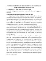
Cobb-Douglas or Translog?

Prob > F = 0.0071

F( 6, 4154) = 2.95

( 6) lout_npk = 0

( 5) lout_urea = 0

( 4) lp_urea_npk = 0

( 3) loutput2 = 0

( 2) lp_npk2 = 0

( 1) lp_urea2 = 0

</div>
(42)<div class='page_container' data-page=42>

Testing linear homogeneity of the

Translog cost function

Prob > F = 0.0018

F( 3, 4154) = 5.03

( 3) lout_urea + lout_npk = 0

( 2) lp_urea2 + lp_npk2 + lp_urea_npk = 0

( 1) lp_urea + lp_npk = 1

> */ (lout_urea + lout_npk = 0)

> / (lp_urea2 + lp_npk2 + lp_urea_npk = 0) /

. test (lp_urea + lp_npk = 1) /*

</div>
(43)<div class='page_container' data-page=43>

Imposing linear homogeneity on the

Translog cost function



constraint 1 lp_urea + lp_npk = 1



constraint 2 lp_urea2 + lp_npk2 + lp_urea_npk = 0



constraint 3 lout_urea + lout_npk = 0



cnsreg lcost lp_urea lp_npk loutput lp_urea2

</div>
(44)<div class='page_container' data-page=44>

Imposing linear homogeneity on the

Translog cost function

_cons -1.257867 .5809441 -2.17 0.030 -2.396828 -.1189055
lout_npk -.1345858 .2770172 -0.49 0.627 -.6776877 .4085162
lout_urea .1345858 .2770172 0.49 0.627 -.4085162 .6776877
lp_urea_npk -5.672884 10.25086 -0.55 0.580 -25.77006 14.42429
loutput2 .0106869 .0083695 1.28 0.202 -.0057219 .0270957
lp_npk2 1.937082 5.07915 0.38 0.703 -8.020767 11.89493
lp_urea2 3.735802 5.236984 0.71 0.476 -6.531487 14.00309
loutput .7192963 .1365959 5.27 0.000 .4514953 .9870973
lp_npk 6.290339 3.880915 1.62 0.105 -1.31833 13.89901
lp_urea -5.290339 3.880915 -1.36 0.173 -12.89901 2.31833

lcost Coef. Std. Err. t P>|t| [95% Conf. Interval]

( 3) lout_urea + lout_npk = 0

( 2) lp_urea2 + lp_npk2 + lp_urea_npk = 0
( 1) lp_urea + lp_npk = 1

</div>
(45)<div class='page_container' data-page=45>

Translog cost with cost share equation

snpk 4164 3 .3089158 0.0133 57.27 0.0000
lcost 4164 9 .8416739 0.5001 10431.41 0.0000

Equation Obs Parms RMSE "R-sq" chi2 P

Three-stage least-squares regression

> */ (snpk lp_npk lp_urea loutput), constraint(4 5 6 7)

. reg3 (lcost lp_urea lp_npk loutput lp_urea2 lp_npk2 loutput2 lp_urea_npk lout_urea lout_npk) /*
. constraint 7 [snpk]loutput = [lcost]lout_npk

. constraint 6 [snpk]lp_urea = [lcost]lp_urea_npk
. constraint 5 [snpk]lp_npk = [lcost]lp_npk2/2
. constraint 4 [snpk]_con = [lcost]lp_npk

. gen snpk = npk*p_npk/cost

. * Generating cost share for npk

</div>
(46)<div class='page_container' data-page=46>

Translog cost with cost share equation

lp_urea_npk lout_urea lout_npk

Exogenous variables: lp_urea lp_npk loutput lp_urea2 lp_npk2 loutput2
Endogenous variables: lcost snpk

_cons 1.116778 .1409364 7.92 0.000 .8405478 1.393008
loutput .0089511 .0051982 1.72 0.085 -.0012372 .0191393
lp_urea -.3792256 .065678 -5.77 0.000 -.5079522 -.2504991
lp_npk .0304985 .0428719 0.71 0.477 -.0535289 .1145258
snpk

_cons -20.84974 5.387569 -3.87 0.000 -31.40918 -10.2903
lout_npk .0089511 .0051982 1.72 0.085 -.0012372 .0191393
lout_urea -.1963716 .1491281 -1.32 0.188 -.4886574 .0959141
lp_urea_npk -.3792256 .065678 -5.77 0.000 -.5079522 -.2504991
loutput2 .0064543 .0085096 0.76 0.448 -.0102242 .0231328
lp_npk2 .0609969 .0857438 0.71 0.477 -.1070579 .2290517
lp_urea2 -2.505675 .7265642 -3.45 0.001 -3.929715 -1.081635
loutput 1.238252 .4167321 2.97 0.003 .421472 2.055032
lp_npk 1.116778 .1409364 7.92 0.000 .8405478 1.393008
lp_urea 14.70696 3.820055 3.85 0.000 7.219785 22.19412
lcost

</div>
(47)<div class='page_container' data-page=47>

Testing homogeneity

Prob > chi2 = 0.0009

chi2( 3) = 16.38

( 3) [lcost]lout_urea + [lcost]lout_npk = 0

( 2) [lcost]lp_urea2 + [lcost]lp_npk2 + [lcost]lp_urea_npk = 0

( 1) [lcost]lp_urea + [lcost]lp_npk = 1

> */ (lout_urea + lout_npk = 0)

> / (lp_urea2 + lp_npk2 + lp_urea_npk = 0) /

. test (lp_urea + lp_npk = 1) /*

</div>
(48)<div class='page_container' data-page=48>

Imposing homogeneity

snpk 4164 3 .3089154 0.0133 69.54 0.0000
lcost 4164 6 .8430911 0.4984 10572.17 0.0000

Equation Obs Parms RMSE "R-sq" chi2 P

Three-stage least-squares regression

> */ (snpk lp_npk lp_urea loutput), constraint(4 5 6 7 8 9 10)

. reg3 (lcost lp_urea lp_npk loutput lp_urea2 lp_npk2 loutput2 lp_urea_npk lout_urea lout_npk) /*
. constraint 10 [lcost]lout_urea + [lcost]lout_npk = 0

. constraint 9 [lcost]lp_urea2 + [lcost]lp_npk2 + [lcost]lp_urea_npk = 0
. constraint 8 [lcost]lp_urea + [lcost]lp_npk = 1

</div>
(49)<div class='page_container' data-page=49>

Imposing homogeneity

lp_urea_npk lout_urea lout_npk

Exogenous variables: lp_urea lp_npk loutput lp_urea2 lp_npk2 loutput2
Endogenous variables: lcost snpk

_cons 1.16657 .1309565 8.91 0.000 .9099001 1.42324
loutput .0084214 .0051685 1.63 0.103 -.0017087 .0185515
lp_urea -.388852 .065142 -5.97 0.000 -.516528 -.2611761
lp_npk .0201149 .0410971 0.49 0.625 -.0604339 .1006637
snpk

_cons -1.5325 .4902529 -3.13 0.002 -2.493378 -.5716221
lout_npk .0084214 .0051685 1.63 0.103 -.0017087 .0185515
lout_urea -.0084214 .0051685 -1.63 0.103 -.0185515 .0017087
lp_urea_npk -.388852 .065142 -5.97 0.000 -.516528 -.2611761
loutput2 .0082655 .0077823 1.06 0.288 -.0069875 .0235185
lp_npk2 .0402298 .0821942 0.49 0.625 -.1208678 .2013275
lp_urea2 .3486222 .0628382 5.55 0.000 .2254615 .4717829
loutput .7699614 .1236369 6.23 0.000 .5276375 1.012285
lp_npk 1.16657 .1309565 8.91 0.000 .9099001 1.42324
lp_urea -.1665701 .1309565 -1.27 0.203 -.4232402 .0900999
lcost

</div>

Bài 7: Hàm chi phí và lợi nhuận

THE DUALITY APPROACH:

COST AND PROFIT

FUNCTIONS

The primal vs duality approach

Derivation of cost and profit function

Production Economics



optimal allocation of resources in the production of

goods and services given



technology



resource constraints



output demand (and thus prices of outputs)



prices of inputs



Basic issues:



optimal input uses

The primal vs dual approach



Primal approach



optimal input and output levels are obtained by solving

the optimization problem



Dual approach



Inputs demand and output supply functions can be

derived from the dual functions

 

max

<i>x</i>

<i>pf x</i>



<i>wx</i>

min

st

 

<i>c</i>

<i>x</i>

<i>wx</i>

<i>y</i>



<i>f x</i>





Problems of the primal approach



endogeneity and simultaneity of the production function

(

<i>need instrumental variables, and more advanced techniques to </i>

<i>fix</i>

)



multicollinearity of inputs in the production function (

<i>may </i>

<i>result in incorrect estimates, sometimes unable to obtain the </i>

<i>estimates</i>

)



for some functional forms, it is hard to obtain input demands

and output supply (

<i>the optimization is not always easy</i>

)

Specification of the cost function



Cost min problem



Lagrangian function



FOCs



Solving FOCs to obtain



Cost function

 