A guide to microsoft excel 2013 for scientists and engineers 2015

®

A Guide to Microsoft Excel 2013
for Scientists and Engineers


®

A Guide to Microsoft Excel 2013
for Scientists and Engineers

Bernard V. Liengme
St. Francis Xavier University, Canada

AMSTERDAM • BOSTON • HEIDELBERG • LONDON
NEW YORK • OXFORD • PARIS • SAN DIEGO
SAN FRANCISCO • SINGAPORE • SYDNEY • TOKYO
Academic Press is an imprint of Elsevier


Academic Press is an imprint of Elsevier
125, London Wall, EC2Y 5AS
525 B Street, Suite 1800, San Diego, CA 92101-4495, USA
225 Wyman Street, Waltham, MA 02451, USA
The Boulevard, Langford Lane, Kidlington, Oxford OX5 1GB, UK
Copyright # 2016 Elsevier Ltd. All rights reserved.
No part of this publication may be reproduced or transmitted in any form or by any means, electronic or mechanical,
including photocopying, recording, or any information storage and retrieval system, without permission in
writing from the publisher. Details on how to seek permission, further information about the Publisher’s
permissions policies and our arrangements with organizations such as the Copyright Clearance Center and the
Copyright Licensing Agency, can be found at our website: www.elsevier.com/permissions.

This book and the individual contributions contained in it are protected under copyright by the Publisher (other than
as may be noted herein).
Notices

Knowledge and best practice in this field are constantly changing. As new research and experience broaden our
understanding, changes in research methods, professional practices, or medical treatment may become necessary.
Practitioners and researchers must always rely on their own experience and knowledge in evaluating and using any
information, methods, compounds, or experiments described herein. In using such information or methods they
should be mindful of their own safety and the safety of others, including parties for whom they have a professional
responsibility.
To the fullest extent of the law, neither the Publisher nor the authors, contributors, or editors, assume any
liability for any injury and/or damage to persons or property as a matter of products liability, negligence or otherwise,
or from any use or operation of any methods, products, instructions, or ideas contained in the material herein.
British Library Cataloguing in Publication Data
A catalogue record for this book is available from the British Library
Library of Congress Cataloging-in-Publication Data
A catalog record for this book is available from the Library of Congress
For information on all Academic Press publications
visit our website at
ISBN: 978-0-12-802817-9


Preface
This book is for people in technical fields, students and professionals alike. Its aim is to show the
usefulness of Microsoft® Excel in solving a wide range of numerical problems. Excel does not
compete with the major league symbolic mathematical environments such as Mathematica,
Mathcad, Maple, and the like. Rather it complements them. Excel is more readily available
and is easier to learn. Furthermore, it generally has better graphing features and ways of handling large datasets.
The examples have been taken from a range of disciplines but require no specialized knowledge,
so the reader is invited to try them all. Do not be put off by an exercise that is not in your area of

interest. Each exercise is designed to introduce and explain an Excel feature. The two modeling
chapters will help you learn how to develop worksheets for a variety of problems.
This is very much a practical book designed to show how to get results. The problem sets at the
ends of the chapters are part of the learning process and should be attempted. Many of the questions are answered in the last chapter. The Guide is suitable for use as either a textbook in a
course on scientific computer applications, a supplementary text in a numerical methods course,
or a self-study book. Professionals may find Excel useful to solve one-off problems rather than
writing and debugging a program, or for prototyping and debugging complex programs. A few
topics are not covered by the Guide, such as database functions and making presentation worksheets. These are fully covered in Excel books targeted at the business community, and the techniques are applicable to any field.
I was agreeably surprised by the warm reception given to the first and subsequent editions of the
Guide. I am grateful for the many e-mailed comments and suggestions from readers and academics. This edition has involved a major rewrite since Excel 2013 has several features that
differ from earlier versions. The opportunity has been taken to add new exercises and problems.
I wish again to thank David Ellert, John Quinn, and Robert van den Hoogen for their earlier
assistance. I am honored that Microsoft awarded me the Most Valuable Professional in Excel
in 2014 for the eighth consecutive year. My final thanks go to my wife Pauline for her encouragement and word skills; without her, this book would never have seen the light of day. However, I claim responsibility for all errors and typos.
I welcome e-mailed comments and corrections, and will try to respond to them as soon as I can.
Please check my web site and the Guide’s companion web site />9780128028179/ for supplementary material.
I hope you enjoy learning to “excel.”
Bernard V. Liengme

http:/people.stfx.ca/bliengme

xi


xii

Preface

CONVENTIONS USED IN THIS BOOK
Information boxes in the margins are used to convey additional information, tips, shortcuts, and

the like.
A distinctive font is used for data that the user is expected to type. This avoids the problems of
using quotes. For example: In cell A1, enter the text Resistor Codes. Italics are used for new terms, to
highlight Excel commands, for emphasis, and to avoid the confusion sometimes associated with
quotation marks. Nonprinting keys are shown with a graphical font. For example, rather than
asking the reader to press the Control and Home keys, we use text such as: Press . When
two keys are shown separated by +, the user must hold down the first key while tapping
the second.
An asterisk against a problem number at the end of a chapter indicates that a solution is given at
the end of the book. Excel files for some answered problems and additional files may be found
on the companion web site: />

(VARIABLE ERROR - unrecognised syntax)dotfd"

Chapter

1

Welcome to Microsoft Excel 2013
®

CHAPTER CONTENTS

Exercise 1: Customizing the QAT 5
Exercise 2: Customizing the Ribbon Control 6
The Worksheet 6
Excel 2013 Specifications and Limits 9
Compatibility with Other Versions 9
Exercise 3: The Status Bar 9

When Microsoft Excel is started, you are presented with a window similar to
that in Figure 1.1. From there, you may (i) select from the left panel a
recently opened workbook, (ii) click on Open Other Workbooks, or (iii)
click on the icon Blank workbook to start a new project. Note that while
in Word, we speak of a document, in Excel, we use the term workbook.
In either case, we are referring to a file. In this chapter, we shall not explore
using SkyDrive (now renamed by Microsoft to OneDrive) so we can ignore
the Sign in option in the top right corner.
When we open a new workbook, we have a window showing the Excel interface. Figure 1.1 is a screen capture from the author’s computer with the
Excel window “restored down” to occupy about half of the monitor screen.
The Excel window on your computer may differ slightly depending on your
monitor size and resolution.
It is helpful to know the correct name for the various parts of the window.
This makes using the Help facility more productive and aids in conversing
with other users. As a new term is introduced, it is displayed in italics, and
the reader should try to remember the meaning of such terms.
It is recommended that you read this chapter while seated at the computer
key will back
and experiment as you read it. Remember that pressing the
you out of an action you do not wish to pursue.

A Guide to Microsoft Excel 2013 for Scientists and Engineers
# 2016 Elsevier Ltd. All rights reserved.

1


2 CHAPTER 1 Welcome to Microsoft Excel 2013

n FIGURE 1.1

Title bar: This is at the very top of the window. To the left is the Quick
Access Toolbar (QAT), which is described below. In the center, we have
the name of the currently opened file together with the word Excel. To
the right are a button to activate the Help facility, a button to control how
the Ribbon is displayed, and the three controls to minimize, restore, and
close the Excel window.
Quick Access Toolbar (QAT): When Excel 2013 is first installed, the
QAT holds the commands Save, Undo, and Redo. However, it may be customized to hold others. Furthermore, one can change the location of the
QAT from above the ribbon to below the ribbon. Click on the launcher
at the far right of the QAT to open the QAT customization
button
dialog box.

Warning regarding Undo: Excel
keeps a single undo stack. This
means that if you issue an undo
command, you may undo
changes made to worksheets
other than the currently active
one. If more than one
workbook is open, you may
even undo an action in another
workbook.

As you work through this chapter, you will be asked to save Excel files. It is
strongly recommended that you create a separate folder (perhaps called
tool on the QAT, disExcel Practice) in which to keep these. The first
playing an icon of a floppy disk (something no one uses anymore!), will
open the File Explorer where you can make folders and save files.

Ribbon: The Ribbon stretches across the window under the title bar. It consists of a number of tabs (File, Home, Insert, Page Layout, etc.). The Ribbon
in Figure 1.2 has the Home tab selected. The appearance of a tab will change
with the amount of space allocated to the Excel window. Each tab, other than
File, contains commands displayed in groups. A command is activated by
clicking on its icon. In Figure 1.2, the Home tab is open—note the box


Welcome to Microsoft Excel 2013 3

n FIGURE 1.2

around Home. The Home tab holds mainly formatting commands. Use the
mouse to open another tab by clicking it. We will learn in a later chapter how
to add the Developer tab to the Ribbon. Additional tabs (contextual tabs) get
displayed when you are performing certain operations; for example, the
Charts tab appears when you are working on a chart. Other tabs may appear
after you install certain software.
Some groups have a launch button on their far right and some command
icons have a similar button . In each case, clicking on one of these buttons
expands the choice of commands available to the user. We shall discuss
these on an as-needed basis.
File tab: This tab (the only one to have a color) gives the user access to the
so-called backstage to do things like open, save, or print a file. It also gives
us access to the Options dialog box where we can customize certain Excel
features. We will look at this in later chapters.
Title bar tools: To the far right of the Title Bar, we have five icons
.
Help facility: Clicking the first icon opens the Microsoft Excel Help
dialog box. By default, this connects you to the online help facility at the
Microsoft Excel 2013 site. Unless you are a power user, it is advised that

you skip over any article in Help that has the term DAX (Data Analysis
Expressions) in its title.


4 CHAPTER 1 Welcome to Microsoft Excel 2013

Ribbon Control: By default, the Ribbon displays tabs, their groups, and
gives us the options of both tabs
commands. The Ribbon Control tool
and commands, showing only the tab or having the Ribbon autohide.
The second two options are useful when the user needs to see more of the
working area of the window.
Minimize, Maximize, and Close: The last three buttons are familiar to
all users of Microsoft products and need no further explanation.
Formula Bar and Name Box: Just under the Ribbon is the Formula Bar with
the Name Box to the left. In Figure 1.2, the Name Box is displaying E6. You
will notice that both the E column and the 6 row headings are highlighted and
that the cell at the intersection of this column and row is picked out by a border.
We call E6 the active cell, and we say that the Name Box displays the reference
(or address) of the active cell. When the active cell contains a literal (text or
number), the Formula Bar also displays the same thing, but when the cell holds
a formula, then the Formula Bar displays the actual formula while the cell generally displays the result of that formula. Quick experiment: Type B4 in the
; note how this takes you to cell B4.
Name Box and press

Note: It is becoming common
to talk about tabs when
worksheets are meant. This is
very poor practice since it can
cause confusion and will not

benefit a user searching in
Help.

Worksheet window: The worksheet window occupies most of the Excel
space. A workbook (i.e., a single Excel file) may contain worksheets and
chart sheets (collectively called sheets); we will concentrate on worksheets
for now. A worksheet is divided into rows (horizontally) and columns
(vertically); the intersection of a row and a column is called a cell.
Sheet tabs: Below the worksheet window, we have tools to navigate from
sheet to sheet and to scroll a sheet horizontally. By default, Excel 2013 opens
a new workbook with one worksheet; this number can be changed in the
Options setting. To the left of the first sheet

tab are arrows for navigat-

ing from sheet to sheet; but merely clicking a sheet tab is the most rapid way.
To the right of the last sheet tab is a tool to insert a new worksheet. To the
right of the sheet tabs is the horizontal scroll tool; the vertical scroll tool is on
the right side of the worksheet. We will see later how to rename sheets. If
your mouse has a wheel, you can use it to scroll up and down a worksheet.
Status bar: At the very bottom of the Excel window, we have the status bar.
To the left is the mode indicator. When you move to a cell, this displays
READY; when you start typing, it becomes ENTER; if you double click a
cell (or press the F2 key), it becomes EDIT. Other status conditions like
POINTING and Copy/Paste will be discussed later. We will ignore the second tool (macro recorder) for now. To the right, just before the Zoom tool,
we have Workbook Views buttons that let us display the worksheet in different
ways—Normal, Page Break Preview, Page Layout, and Custom Views (more
on this topic later). Finally, there is Zoom tool that enlarges/reduces the display. You can also change the magnification of the worksheet by rotating the
key.
mouse wheel while holding down the

Exercise 1: Customizing the QAT 5

If we experiment with the Workbook Views buttons, we may notice that the
worksheet gets vertical and horizontal dotted lines. These show how much
will fit on a printed page. Right-clicking the status bar brings up a dialog box
that allows you to customize the status bar. We will show more features of
the status bar in Exercise 3.

EXERCISE 1: CUSTOMIZING THE QAT
Any of the Excel commands can be reached by opening the appropriate tab
and locating the command within one of the tab groups. If there is an operation that you perform frequently, it is convenient to be able to access it from
the QAT, which explains its name. As a demonstration, we will add the
Open command to the QAT:
a. Start Excel and let the mouse pointer hover over the QAT launch button
, which is always the last item on the QAT. A screen tip box will open
with the text Customize Quick Access Toolbar.
b. Now click on the launch button to open the dialog box as shown in
Figure 1.3. On this dialog box, we see the more commonly needed
commands. To add one of the common items to the QAT, just click on it
to bring up a check mark. Correspondingly, click on an item with a check
mark to remove it. The dialog box closes immediately so it must be
reopened to make further selections.
c. If the command you need is not shown, then click on More
Commands. . . to bring up a second dialog box (Figure 1.4). To add a
command to the QAT, select an item in the left panel and click the Add
button. To remove a command, click it in the right panel and click the
Remove button. Locate the Copy command and add it to the QAT. Close
the dialog box by clicking the OK button (or Cancel button to correct a

mistake).
d. There is little merit in having the Copy command on the QAT since there
is a very convenient shortcut ( +C) for this purpose. Right click on the
Copy command on the QAT (it looks like two sheets of paper) and use
the Remove command in the pop-up menu.
e. It is sometimes said, tongue in cheek, that there are always three ways of
doing the same thing in Excel! To demonstrate that this is not too great
an exaggeration, open the File tab, on the left side, and locate and click
on Options. This opens a dialog box; click on QAT in the left panel. This
again brings us to the dialog box shown in Figure 1.4. Close the dialog
box by clicking the Cancel button.
As you become more familiar with Excel, we will condense the second and
third sentences in the above to the simple instruction: use File / Options /
Quick Access Toolbar.

Note: If a Print command is
needed on the QAT, it is
recommended that one uses
Print Preview and Print rather
than Quick Print. This lessens
the risk of wasting paper at
home or mistakenly printing
confidential material in an
office setting environment.

Note: The procedure above
shows how to add any
command to the QAT, but there
is a much simpler method for
commands that are already on

the Ribbon. Just right click the
command icon and select Add
to Quick Access Toolbar.


6 CHAPTER 1 Welcome to Microsoft Excel 2013

n FIGURE 1.3

n FIGURE 1.4

EXERCISE 2: CUSTOMIZING THE RIBBON CONTROL
The Ribbon may be customized using the steps discussed in (c), but this is
not a suitable topic for this chapter. Rather, we shall change how the entire
Ribbon is displayed, not what commands are displayed on it:
. Click on it
a. To the right on the Title Bar is the Ribbon Control tool
and experiment with the three options.
b. In your own words, state how the Ribbon behaves with (i) Auto-hide,
(ii) Show Tabs, and (iii) Show Tabs and Commands. What are the
advantages/disadvantages of each setting?

THE WORKSHEET
The worksheet window is the heart of the Excel application. It is here that we
enter and work with data. It is helpful to learn some terms.
Columns and rows: A worksheet is divided vertically into columns and
horizontally into rows. The intersection of a column and row forms a cell.
At the top of the worksheet, we have the column headers (the letters A, B, C,
etc.) and to the left the row headers (the numbers 1, 2, 3, etc.). The last

The Worksheet 7

column is XFD (there are 16,384 columns); the last row is numbered
1,048,576; thus, a single sheet has some 17 billion cells. Your computer
would need to have a very large amount of memory if you planned to fill
every cell.
Cell: A cell is the unit on the worksheet; it may be empty or it may hold
data. Generally, cells are outlined by gridlines. However, it is possible to
request Excel not to display gridlines for a particular worksheet. Note
that gridlines are not printed unless otherwise specified in Page Layout /
Sheet Options.
Active cell: If you click on a single cell on the worksheet, it is displayed with
a solid border. We call this the active cell. The reference (such as A1) of the
active cell is displayed in the Name Box. The correct term for the combination of column letter and row number (as in A1) is reference, but address is
acceptable. What is not acceptable is name since this has a very special
meaning in Excel. It is possible to configure Excel to use another reference
system in which the top left cell is referred to as R1C1 but we shall not be
concerned with that method. As noted above, the Name Box displays the
reference of the active cell.
Range: A range is a group of contiguous cells. The shaded areas (see
Figure 1.5) B2:B109, D2:G2, D5:F9, and H8 are examples of ranges. Technically, a single cell is also a range—it is a range consisting of just one cell.
We refer to a range using the addresses of the top left cell and the bottom
right cell separated by a colon.
Data and Formulas: A cell may contain either data or a formula. Data and
formulas are frequently entered by typing in the cell. You can complete
key, pressing
(commit) your entry in a number of ways: pressing Enter

n FIGURE 1.5

8 CHAPTER 1 Welcome to Microsoft Excel 2013

one of the arrow keys ( , , , or ) or the Tab key
, or clicking the
checkmark ( ) to the left of the Formula Bar. There is another method—
clicking on another cell—but this is a very poor habit to pick up since
the result when entering a formula is generally not what you want! The
key generally takes you down to one cell below, but we can change this
with an option setting to move one to the right. Data and formulas can also
be placed in cells by copying (or cutting) them from other cells and then
using the Paste command. The source cells can be in the same worksheet
or in another worksheet or even from another workbook.
Data: The data we enter into a cell can be one of four types. It could be text
(such as the word Experiment), a number (123.45), a date (1/1/2013), or a
Boolean constant (TRUE or FALSE). Later, we shall see that a date is actually a number with a special format applied.
Formulas: A formula always begins with an equals sign (¼) followed by a
combination of constants and cell references (e.g., ¼2*1.2345 and ¼2*A2).
It may also contain one or more functions (e.g., ¼SUM(A1:A10) and
¼4*MAX(A1:A5)+2). A formula normally displays a value in the cell;
this can be any one of the data types listed above. So the cell containing
the formula may display a value such as 6.28318, but when it is the active
cell, the Formula Bar may display the formula ¼2*PI(). If the formula fails,
it may display (we say it returns) an error value. We start to use formulas in
Chapter 2.
Formatting: This is the term used to describe changing how the value in a
cell is displayed. We may format a cell to alter the font (typeface, size, or
color) and to add a border or a fill color. By far, the most important aspect of
this topic relates to numbers. In a newly opened worksheet, every cell is formatted in what is called General. If I type 1.23456789 into a cell, I may see

1.234568 because the combination of column width and font size allows just
seven digits and the decimal. So my entry is rounded. The Formula Bar will
display the actual number 1.23456789. We may widen the cell to display
more digits. This rounding occurs only with real numbers (numbers having
decimal parts) and not with integer numbers. If I type 1234567890, Excel
will widen the cell, but when more digits are used, as in 123456789012,
Excel displays it in scientific notation as 1.234567E + 11 (meaning
1.234567 Â 1011). Had the column been formatted to a narrow width beforehand, the result would show fewer digits. We will see later that we may
change the format of a number. What is important to remember is that
changing the format does not alter the actual stored value. We examine this
in a later exercise, but it is good to learn early that there are stored values and
displayed values.


Exercise 3: The Status Bar 9

EXCEL 2013 SPECIFICATIONS AND LIMITS
As with the vast majority of Windows mathematical applications, Excel is
limited to a 15 decimal precision. That means you cannot store a 16-digit credit
card number as a number in Excel, but since it is not actually a number (you
never perform any arithmetic operations on a credit card number), the solution
is to store it as text by typing a single quote (apostrophe) before the number.
More importantly, Excel appears to get some math slightly wrong; we examine
this topic when we look at the IEEE 756 convention in Chapter 2.
In earlier version of Excel, if you typed specifications in the Help query box,
you were shown all sorts of details: What is the size of the largest number
that can be stored? (9.99999999999999E + 307) What is the maximum
width of a column? (255 characters). Likewise, you could find that the maximum number of worksheets in a workbook is limited by the size of the computer memory. Currently, the specifications for Excel 2013 are not available
on any website, but shows the specifications and
limits for Excel 2010, and these have remained unchanged.

COMPATIBILITY WITH OTHER VERSIONS
Some people are still using Office 2003 so we need to know how to communicate with them. Starting with Office 2007, Microsoft made a radical
change to the format of Office files, even the extensions changed. So an
Excel 2003 user cannot open workbook generated in one of the newer versions (e.g., an Excel file with the extension XLSX) unless the Microsoft
Office Compatibility pack is installed on the computer. Alternatively, an
Excel 2013 user may save a workbook in the older file format making a file
with the extension XLS. However, neither of these methods will help if the
original Excel 2013 file made use of new features (e.g., advanced conditional formatting) or functions introduced since Excel 2003 (e.g., Unicode).
One can open an old Excel file (extension XLS) in Excel 2013. The title bar
will include the phrase Compatibility Mode. The reader should also be aware
that both Excel 2010 and Excel 2013 introduced new features and functions.
So opening an Excel 2010 file in Excel 2007 or an Excel 2013 file in either
Excel 2007 or Excel 2010 can result in problems.

EXERCISE 3: THE STATUS BAR
Open an Excel workbook, and on Sheet1 in A1:A10, type some numbers.
Now, using the mouse, select A1:A10. The status bar should display to
the right something like that shown in Figure 1.6. If this is not shown, right


10 CHAPTER 1 Welcome to Microsoft Excel 2013

n FIGURE 1.6

click the status bar to bring up its customization dialog box and put check
marks in the required boxes with the mouse.
Note also that one can have the status bar display Caps when Caps Lock is
on. The reader may wish to experiment with other options on the status bar.

PROBLEMS
If you like puzzle solving, try these problems. We will be covering the topics
in the subsequent chapters, but you may enjoy the challenge:
1.

Type your name in any cell. Make it bold and italic. Can you find how
to remove bold or italic?

2.

key. It should show the
In cell D1, enter 5TODAY( ) and press
current date. Maybe it displays something like 15/3/2013 (or 3/15/
2013 if your Windows Regional Settings specifies the American date
format); can you change it to March 15, 2013? Hint: Look in the Home
/ Number group.

3.

Copy the cell with your name. Paste it in another cell. Copy the cell
with the date. Note the “ant track” running around the cell you copied.
If you double click an empty cell, the track disappears and you can no
longer paste. You have been using the Windows clipboard. Now click
the Clipboard launcher on the Home tab (far left). This opens the
Office Clipboard, which can hold more than one item. Experiment
with it.

4.

key. This gives an

In A5, type the formula 522/7 and press the
approximate value for π. Can you discover how to make this display
with eight decimal places?

5.

Type some numbers in cells D1 to D5—later, we will give this
instruction as “put numbers in D1:D5.” Click D6—or, in technical
terms, make D6 the active cell. Look for the Σ icon (it is in Home /
Editing). Click it to see what happens.


Chapter

2

Basic Operations
CHAPTER CONTENTS

Exercise 1: Simple Arithmetic 12
Exercise 2: The Mathematical Operators 14
Exercise 3: Formatting (Displayed and Stored Values) 16
Exercise 4: Working with Fractions 17
Exercise 5: A Practical Worksheet 19
Copying Formulas: What Happens to References? 20
What's in a Name? 22
Exercise 6: Another Practical Example 24
Exercise 7: The Evaluate Formula Tool 27
Special Symbols, Subscripts, and Superscripts 28
Mathematical Limitations of Excel 30

Play It Again, Sam 32

This book is about problem solving so we shall spend little time on the preparation of presentation-worthy worksheets. We will give some information
on how to make a worksheet more readable, but the emphasis is on mathematical operations. The topics in this chapter include
n
n
n
n
n
n
n
n
n
n

entering numbers, including fractions and percentages;
simple formulas such as ¼A1+B1+C1;
range finders (colored borders showing what cells are used in a formula);
arithmetic operators +, À, * , /, and ^ ;
the Evaluate Formula tool;
error values such a #DIV/0! and #VALUE!;
copying with commands and shortcuts;
formatting numbers;
the difference between stored and displayed values;
round-off errors resulting from the IEEE 754 standard.

If you are familiar with an earlier version of Microsoft Excel, you may be
tempted to skip this chapter. You are urged to at least read the exercises to
find out about new Excel 2013 features.
A Guide to Microsoft Excel 2013 for Scientists and Engineers

# 2016 Elsevier Ltd. All rights reserved.

11


12 CHAPTER 2 Basic Operations

EXERCISE 1: SIMPLE ARITHMETIC
Imagine that from time to time, you are given some data consisting of rows
of three numbers and you are asked to find the sum and product of each triple. Of course, this could be done with a simple calculator, but a spreadsheet
offers three advantages: we can reuse our spreadsheet from day to day, we
can see the values we have entered, and we can make a neat printout of the
results. Our completed spreadsheet will look like Figure 2.1:
a. In cells A1 to E1, enter the text shown in Figure 2.1. In A2:C3, enter the
numbers shown. You will note that as you enter the text, it is left aligned
in a cell, while numbers are right aligned.
b. Use the mouse to select A1:E1. On the Home tab, click the right
alignment command in the Alignment group; it is the third command in
the second row of this group.
c. Unless we have used a spreadsheet before, we might be tempted to type
when finished)
51+3+4 in cell D2. Try this (remembering to press
and it will give the correct answer, but this totally ignores the main idea
behind a worksheet. We should not have to retype data. Wherever
possible, formulas should refer to cell values. Click on D2 and tap the
key to remove this formula.
d. Now type 5A2+B2+C2 and click the check mark to the left of the formula
bar when the formula is complete. Notice that, as you type, the status bar
displays ENTER, but once the checkmark tool to the right of the
key) is used to commit the formula, it

formula bar (or the
shows READY.
e. Next, we see another way to build a formula. In D3, type an equals sign
(¼), but rather than typing A3, click the A3 cell. Now type + and
continue building the formula with this pointing method. The status will
alternate between POINT and ENTER. Note how the cells take on a
colored border that matches the colors of the cell references in the
formula (Figure 2.2). Again, click the checkmark to commit the formula
once it is finished. In this case, pointing has little advantage over typing,
but in other cases, it has some advantages. Pointing helps to ensure we
reference the correct cell in a complex worksheet, and it is very useful to
reference a cell on another sheet that could be in another workbook.

A
1
2
3
4
5

B
a
1
4
5
6

n FIGURE 2.1

C

b
3
5
7
8

c
4
6
9
3

D
E
sum product
8
12
15
120
21
315
17
144


Exercise 1: Simple Arithmetic 13

n FIGURE 2.2

n FIGURE 2.3

Of course, we do not have to rebuild the formula for every cell. We can
copy from one cell to another. Here, we look at two ways of doing this,
and a little later, we will see a third (and the fastest) method.
f. The first method uses the Copy and Paste commands located on the
Clipboard group of the Home tab (far left)—see Figure 2.3.
With D3 as the active cell, click the Copy command. Select D4:D5 and
use the Paste command (this is the larger icon on the group). Note how
the cell we copied (D3) has a mobile dotted border. While this “ant
track” is visible, the contents of the cell are still on the Clipboard and
may be copied to any other range or cell. The ant track disappears as
.
soon as you start to edit any cell but can also be removed by pressing
If you allow the mouse pointer to hover over the commands in the Clipboard group, screen tips pop up to tell the purpose and the shortcut key+C and Paste is
+V.
strokes for each command. So Copy is
+C and
g. Delete D3:D5 and repeat the copy-and-paste action using the
+V shortcuts. If you accidentally delete D2, use
+Z to undo the
action.
h. Delete D3:D5 again in preparation for another way to copy D2 down to
D5. Move to D2 and note that the active cell border has a small solid
square in the lower right corner; this is the fill handle. Carefully move
the mouse pointer until it is over the fill handle—the pointer changes
from an open cross to a solid cross. Hold down the left mouse button and
drag the solid cross down to D5. In step (k) below, we shall see yet
another method of filling a range.
For the final stage in this exercise, we look at another approach to building formulas. Rather than typing the formula in the cell, we will type it in
the formula bar. There is an advantage to doing this when the formula is

long, but we shall do it here for demonstration purposes:

Note: The
key may be used
whenever you what to cancel
what you are doing. Also if you
start to edit a cell and wish to
terminate the operation
without making any changes,
you can use the tool located
between the Name Box and the
Formula Bar.

Note: It is customary to show
shortcuts with capital letters
+C but it is not
like
necessary to hold the
key to generate a capital letter
when using a shortcut.


14 CHAPTER 2 Basic Operations

i. Make E2 the active cell. In the formula bar, type 5. Now complete the
formula to be 5A2*B2*C2 either by typing or by pointing. Commit the
or the checkmark on the formula bar. Note that
formula with either
the multiplication operator is an asterisk (*).
Lastly, we will fill in cells E3:E5. With E2 as the

j.

active cell, move the mouse pointer over the fill handle (watch for the change
from open to solid cross) and double-click the fill handle. The formula from
E2 is copied down to E5. This Auto Fill feature can be used with vertical
tables (data arranged in columns) but not with horizontal tables. It can
be used to renew formulas when you make a change to the top cell.
k. Double-click on any cell in the range D2:E5. Note that the status bar
displays EDIT. But more importantly, observe the colored borders around
the cells in the corresponding cells in columns A, B, and C. Excel uses
these range finders to pictorially show you which cells a formula refers to.
l. In A6:C6, type some numbers. When you complete the last entry, Excel
will automatically add the formulas in D6 and E6. This is an example of
Auto Extend. It requires that the table has at least four rows of entries
above the current row. For more information on this topic, see http://
support.microsoft.com/kb/231002.
m. In the QAT, click the Save command (picture of a floppy disc) and save
the file as Chap2.xlsx.

EXERCISE 2: THE MATHEMATICAL OPERATORS
Note: If we had numbers in A1:
A100 to be summed, we would
be ill-advised to start with 5A1
+A2. . . . Rather, we would use
the SUM() function to be
discussed later. There is also
the PRODUCT() function to find
continued multiplications.

The following table lists the arithmetic operators, their symbols, examples,
and order of precedence.
You may not be accustomed to treating the % symbol as an operator; essentially, it means divide the preceding number by 100. Exponentiation, of
course, means raising a number to a certain power.

Operation

Symbol

Examples

Negation
Percentage
Exponentiation
Multiplication
Division
Addition
Subtraction

–
%

À1 and –A1
5%
2^ 3, A1^ 3, A1^ B1
2*3, 2*A1, A1*B1
2/3, A1/3, A1/B1
2+3, A1+3, A1+B1
3À2, A1ÀB1

^

*
/
+
–

Order of Precedence
1
2
3
4
5


Exercise 2: The Mathematical Operators 15

Excel evaluates formulas left to right using the order of precedence. So
¼60À20/5 will yield 56, not 8, since the division precedes the subtraction.
We can override the order of precedence by the use of parentheses. Thus,
¼(60À20)/5 gives 8 because everything within parentheses is done first.
Open the workbook (the Chapter2.xlsx file) made in Exercise 1 by opening
the File tab on the Ribbon and locating Chap2.xlsx in the Recent Document
list. If it does not appear, click on Computer in the center panel to go to your
Documents folder (Figure 2.4):
a. Click the Sheet2 tab (just above the status bar) to open a new worksheet
or, if there is no Sheet2 tab, use the Insert Worksheet tool, which is to the
right of the last tab in the sheet tab list.
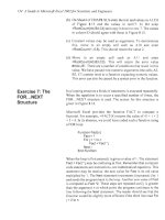
b. Look at Figure 2.5. Mentally compute each result—or at least the
first six.

c. Create a worksheet using the values and formulas shown in Figure 2.5.
Did you get the correct values? How about C5 and C6? Were there any
surprises other than perhaps C7 and C8, which will be discussed shortly?
d. To see how Excel performs a calculation, select each cell in turn and on
the Formulas tab use the Evaluate Formula tool in the Formula Auditing
group. As you press the Evaluate Formula button on the dialog, the
formula is evaluated step by step. This tool is very useful with complex
formulas and it can help you debug your work when you get an
unexpected result—see Exercise 7. You will note that À5^2 is evaluated
as (À5)^2 and not –(5)^2 since negation precedes exponentiation.
e. Save the workbook. You may wish to experiment with the shortcut
+S to do this.

n FIGURE 2.4


16 CHAPTER 2 Basic Operations

A
1
2
3
4
5
6
7
8

B
C

2
-3 =A1+B1
1
2 =2*A2-B2
-1
2 =A1+A2+A3/B3
3
5 =(A1+A2+A3+A4)/B4
5
2 =-A5^B5
-5
2 =-A6^B6
5
5 =A7/(A7-B7)
5 apple
=A8+B8

n FIGURE 2.5

We have not explained the results #DIV/0! in C7 and #VALUE! in C8. These
are examples of error values. In the first evaluation step of the formula in C7,
we get ¼5/0. Division by zero is said by mathematicians to be “undefined” so
Excel tells us this is an error value. A green triangle in the upper-left corner of
a cell indicates an error in the formula in the cell. The Trace Error button
appears when you select the cell. Click the button’s arrow for a list of options
(refer to Figure 2.6). Experiment with this for yourself. You will find that
Ignore Error removes the green triangle, but this reappears if you double-click
without making changes to the formula.
the cell and press
The #VALUE! error in C8 occurs because we are using the wrong data type:

B8 contains a text value that is incompatible with the addition operator. We
will soon discover that the SUM function ignores nonnumeric data, so it can
be used in circumstances when we want to add values in a range, ignoring
any text that happens to be in the range.
In addition to #DIV/0! and #VALUE!, other error values are #REF!, #NUM!,
#NAME?, and #N/A. We will discuss them as we proceed, but for now, note
that each begins with a number (hash or pound) symbol. A worksheet displaying an error value has a mistake in it and needs attention except that #N/A is
often acceptable and is taken to mean “not applicable” or “not available.” Later,
we shall see how conditional formatting may be used to hide error values.
n FIGURE 2.6

In Chapter 5, we meet some conditional functions that enable us to avoid
error values such as #DIV/0! and #N/A in many circumstances.

EXERCISE 3: FORMATTING (DISPLAYED AND
STORED VALUES)
This is a very simple exercise, but it is most important for an Excel user to
know the difference between a displayed and a stored value (Figure 2.7):
a. Open your Chap2.xlsx workbook and move to Sheet3 or insert Sheet3 if
necessary. Type the text shown in the rows 1 and 3 of Figure 2.7. Right
align the entries in A3:C3 as we did in Exercise 1.


Exercise 4: Working with Fractions 17

A
B
C
1 Displayed and Stored Values
2

N
2+N
2*N
3
1.249
3.249
2.498
4
1.25
3.25
2.498
5
n FIGURE 2.7

n FIGURE 2.8

b. In A4 and A5, type the value 1.249. With A5 as the active cell, locate the
Decrease Decimal tool in the Number group of the Home tab (refer to
Figure 2.8). Click this once to have A5 show 1.25. We say that 1.25 is the
displayed value. Note that the formula bar still reports 1.249; this is
the stored value.
c. In B4 and C4, enter the formulas 52+A4 and 52*A4, respectively.
d. In B5 and C5, enter the formulas 52+A5 and 52*A5, respectively. For the
purpose of this exercise, please do not copy them from the row above but
type them in.
e. Save the workbook.
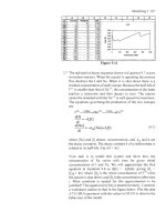
Row 4 has no surprises, but look again at row 5. We know that A5 has the
value 1.249 and that it was formatted to display only two decimal places.
The addition of 2 gives 3.249, while multiplication gives 2.498. C5 displays
the expected value, but B5 has a rounded result. It is a feature of Excel that a

cell with a simple formula (such as ¼A1 which has no arithmetic operator or
¼A1+2 and ¼B1À3 with just the addition/subtraction operators) inherits
the format of the referenced cell. Had we copied the formula from B4 to
B5, the cell would have displayed 3.249.
Note that if you move to A5, the formula bar displays the stored value of
1.249 rather than the formatted value of 1.25. If we had wanted the formula
to treat 1.249 as 1.25, then we could have used the ROUND function as
shown later. Alternatively, we can have Excel treat all numbers to have
the precision of the displayed values. This can be helpful in some financial
accounting work but can lead to some confusion in other cases, so we shall
not pursue this feature.

EXERCISE 4: WORKING WITH FRACTIONS
Most of us work with decimal numbers, but there are still occasions when we
would like to do some arithmetic with fractions. In this exercise, we shall
learn how to enter a number like 2 ¼ and how to have a number such as
14.6667 displayed as 14 10/15:


18 CHAPTER 2 Basic Operations

A
B
C
D
E
F
1 Working with Fractions
2
3 Adding numbers to give an answer to the nearest 1/2

4
4 7/8
3/4
6
11 1/2
5
6 Displaying and adding numbers to give answer in fifteenths
7
3 3/15
6 5/15
5 2/15
14 10/15
n FIGURE 2.9

a. Enter the text shown in A1, A3, and A6 of Figure 2.9.
b. Enter the numbers in A4:C4. The number in A4 is entered by typing the 4
followed by a space and then 7/8. Note that the formula bar displays
4.875. The ¾ is entered as 0 3/4 and Excel helpfully omits the zero. If
you enter only 3/4, Excel will be over helpful and think you mean a date
(3 Apr or 4 Mar of the current year depending on the date format in
regional setting). If C4 has previously held a fractional value before you
enter the 6, then the value will be displayed with spaces following it.
c. In E4, enter ¼A4+B4+C4 by either typing or using the pointing method
mentioned earlier. The result will be displayed as 11 5/8. With E4 as the
active cell, look at the Number group on the Home tab; it is displaying
Fraction; Excel has formatted this cell to reflect the format of the cells
being added.
d. Since we were set the task of having the result in E4 displayed to the
nearest ½, we need to format the cell. Use Home / Number launcher to
open up the Format Cells dialog (Figure 2.10) from where we may select

As halves ½ in the Fraction category and click the OK button.
e. Enter the values in A7:C7 and copy the formula E4 to E7.
f. The result in E7 is actually 14.66667, but it displays as 14 ½ because the
copy action copied both the formula and the format of E5. If you repeat
the instructions of step (d) above, you will find that the only fractions

n FIGURE 2.10


Exercise 5: A Practical Worksheet 19

Excel offers are halves, quarters, sixteenths, tenths, and hundredths. Are
we out of luck in wanting fifteenths? No, all we need to do is move to the
Custom category in the Format Cells dialog and in the Type box replace
# ?/2 by # ?/15. Note that there is a space after the # symbol. Save the
workbook.

EXERCISE 5: A PRACTICAL WORKSHEET
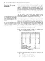
In this exercise, we demonstrate a practical worksheet. An electrical engineer wishes to compute the effective resistance of four resistors in parallel;
refer to Figure 2.11 for a diagram of what is meant by this and for the equation used to compute the answer. You are not expected to make the diagram!
Also ignore the fact that gridlines are not seen and there are borders around
some cells; we will find how to do this shortly:
a. Open Chap2.xlsx and use the Insert Sheet command (last item on the
sheet tab list) to create Sheet4.
b. Enter the text shown in A1, A3, A6, D6, A8, and A9. Enter the values
shown in B3:E3.
c. In B4, enter the formula ¼1/B3 and copy it across to E4 by dragging the
fill handle.
d. In B6, we compute 1/R1+1/R2+1/R3+1/R4 using the formula ¼B4+C4
+D4+E4. You may wish to compose this using the pointing method. We

will see in Chapter 5 how the use of functions can make the worksheet
more useful.
e. In E6, we find the reciprocal of the sum of reciprocals with 51/B6 to give
us Re.
f. In B9, enter the formula ¼1/(1/B3+1/C3+1/D3+1/E3) to demonstrate a
shorter method.
g. Use the Decrease Decimal tool on the Home / Number group to display
E6 and B9 with no decimal places.

A
B
1 Resistors in Parallel
2
3 Resistors
1240
0.00081
4 1/R
5
6 1/Re

0.00207

7
8 Alternative method
9 Re
10

n FIGURE 2.11

482

C

D

1800
0.00056

E

F

2000
4700
0.0005 0.00021
Re

482

G

H

I

J


20 CHAPTER 2 Basic Operations

Note: When a mathematical
formula references a blank cell,
the blank is treated as a zero.

It is dangerous to rely on the results of any computer program (including
an Excel worksheet), which has not been tested. Try your worksheet with
some simple values such as four resistors of 2 Ω or four of 100 Ω. Does
your worksheet agree with the results you computed in your head? This
does not constitute a total validation of the worksheet but it gives us more
confidence in its results.
Does the worksheet have any limitations? Clearly, it cannot be used for
more than four resistors, but that is not a serious drawback from a practical point of view. How about fewer than four?
key. Oh dear, our worksheet displays a
h. Move to E3 and press the
number of #DIV/0! error values. The blank value in E3 is treated as a
zero value. Excel cannot compute the formula in E4 (¼1/E3); this
generates the first #DIV/0! error. The error is carried over to B6, which
tries to use the result in E4, and then to E7, which tries to use the B6
value. B9 also attempt to compute1/E3 and generates its own #DIV/0!
error.
Let’s think about the physical meaning of removing a resistor. It does not
mean inserting a resistor of 0 Ω; that would be a short circuit. Rather, it
means replacing R4 by a very large resistance since air is a nonconductor.
So we might solve our problem with a large number such as 1 MΩ.
i. Enter values of 2 for the first three resistors and 1E6 (you may be
familiar with this notation meaning 1 Â 106 from your hand
calculator) for the last one. Now compute the expected results in
your head. Does the worksheet give a good answer? Of course, if
the first three resistors have very big values, then our missing R will
need to be very large, say 1E100. This is another problem we can

solve more efficiently with functions as we will see in Chapter 5.
j. Save your workbook.

COPYING FORMULAS: WHAT HAPPENS TO
REFERENCES?
We have seen in the last exercise that when the formula ¼1/B3 was
copied from B4 to C4, the formula was adjusted to ¼1/C3. This is very
useful, but there are times when we want something else. First, we need
to understand how Excel goes about adjusting references when you copy
a formula.
The formula in B4 was ¼1/B3; think of this as meaning ¼1 / (the cell that in
the same column, one row above). This is what is meant by a relative address.
The reference to B3 is interpreted relative to the cell that holds the formula. So
when we copy this to C4, it is still ¼1 / (the cell that in the same column, one