Tài liệu Independent component analysis P2 pptx
Bạn đang xem bản rút gọn của tài liệu. Xem và tải ngay bản đầy đủ của tài liệu tại đây (997.06 KB, 43 trang )
Part I
MATHEMATICAL
PRELIMINARIES
Independent Component Analysis. Aapo Hyv
¨
arinen, Juha Karhunen, Erkki Oja
Copyright
2001 John Wiley & Sons, Inc.
ISBNs: 0-471-40540-X (Hardback); 0-471-22131-7 (Electronic)
2
Random Vectors and
Independence
In this chapter, we review central concepts of probability theory,statistics, and random
processes. The emphasis is on multivariate statistics and random vectors. Matters
that will be needed later in this book are discussed in more detail, including, for
example, statistical independence and higher-order statistics. The reader is assumed
to have basic knowledge on single variable probability theory, so that fundamental
definitions such as probability, elementary events, and random variables are familiar.
Readers who already have a good knowledge of multivariate statistics can skip most
of this chapter. For those who need a more extensive review or more information on
advanced matters, many good textbooks ranging from elementary ones to advanced
treatments exist. A widely used textbook covering probability, random variables, and
stochastic processes is [353].
2.1 PROBABILITY DISTRIBUTIONS AND DENSITIES
2.1.1 Distribution of a random variable
In this book, we assume that random variables are continuous-valued unless stated
otherwise. The cumulative distribution function (cdf) of a random variable at
point is defined as the probability that :
(2.1)
Allowing to change from to defines the whole cdf for all values of .
Clearly, for continuous random variables the cdf is a nonnegative, nondecreasing
(often monotonically increasing) continuous function whose values lie in the interval
15
Independent Component Analysis. Aapo Hyv
¨
arinen, Juha Karhunen, Erkki Oja
Copyright
2001 John Wiley & Sons, Inc.
ISBNs: 0-471-40540-X (Hardback); 0-471-22131-7 (Electronic)
16
RANDOM VECTORS AND INDEPENDENCE
σσ
m
Fig. 2.1
A gaussian probability density function with mean and standard deviation .
. From the definition, it also follows directly that ,and
.
Usually a probability distribution is characterized in terms of its density function
rather than cdf. Formally, the probability density function (pdf) of a continuous
random variable is obtained as the derivative of its cumulative distribution function:
(2.2)
In practice, the cdf is computed from the known pdf by using the inverse relationship
(2.3)
For simplicity, is often denoted by and by , respectively. The
subscript referring to the random variable in question must be used when confusion
is possible.
Example 2.1 The gaussian (or normal) probability distribution is used in numerous
models and applications, for example to describe additive noise. Its density function
is given by
(2.4)
PROBABILITY DISTRIBUTIONS AND DENSITIES
17
Here the parameter (mean) determines the peak point of the symmetric density
function, and (standard deviation), its effective width (flatness or sharpness of the
peak). See Figure 2.1 for an illustration.
Generally, the cdf of the gaussian density cannot be evaluated in closed form using
(2.3). The term in front of the density (2.4) is a normalizing factor that
guarantees that the cdf becomes unity when . However, the values of the
cdf can be computed numerically using, for example, tabulated values of the error
function
erf
(2.5)
The error function is closely related to the cdf of a normalized gaussian density, for
which the mean
and the variance . See [353] for details.
2.1.2 Distribution of a random vector
Assume now that is an -dimensional random vector
(2.6)
where denotes the transpose. (We take the transpose because all vectors in this book
are column vectors. Note that vectors are denoted by boldface lowercase letters.) The
components of the column vector are continuous random variables.
The concept of probability distribution generalizes easily to such a random vector.
In particular, the cumulative distribution function of is defined by
(2.7)
where again denotes the probability of the event in parentheses, and is
some constant value of the random vector . The notation means that each
component of the vector is less than or equal to the respective component of the
vector . The multivariate cdf in Eq. (2.7) has similar properties to that of a single
random variable. It is a nondecreasing function of each component, with values lying
in the interval . When all the components of approach infinity,
achieves its upper limit ; when any component , .
The multivariate probabilitydensity function of is defined as the derivative
of the cumulative distribution function with respect to all components of the
random vector :
(2.8)
Hence
(2.9)
18
RANDOM VECTORS AND INDEPENDENCE
where is the th component of the vector . Clearly,
(2.10)
This provides the appropriate normalization condition that a true multivariate proba-
bility density must satisfy.
In many cases, random variables have nonzero probability density functions only
on certain finite intervals. An illustrative example of such a case is presented below.
Example 2.2 Assume that the probability density function of a two-dimensional
random vector = is
elsewhere
Let us now compute the cumulative distribution function of . It is obtained by
integrating over both and , taking into account the limits of the regions where the
density is nonzero. When either or , the density and consequently
also the cdf is zero. In the region where and , the cdf is given
by
In the region where and , the upper limit in integrating over
becomes equal to 1, and the cdf is obtained by inserting into the preceding
expression. Similarly, in the region and , the cdf is obtained by
inserting to the preceding formula. Finally, if both and ,the
cdf becomes unity, showing that the probability density has been normalized
correctly. Collecting these results yields
or
and
2.1.3 Joint and marginal distributions
The joint distribution of two different random vectors can be handled in a similar
manner. In particular, let be another random vector having in general a dimension
different from the dimension of . The vectors and can be concatenated to
EXPECTATIONS AND MOMENTS
19
a "supervector" = , and the preceding formulas used directly. The cdf
that arises is called the joint distribution function of and , and is given by
(2.11)
Here
and are some constant vectors having the same dimensions as and ,
respectively, and Eq. (2.11) defines the joint probability of the event and
.
The joint density function
of and is again defined formally by dif-
ferentiating the joint distribution function with respect to all components
of the random vectors and . Hence, the relationship
(2.12)
holds, and the value of this integral equals unity when both and .
The marginal densities of and of are obtained by integrating
over the other random vector in their joint density :
(2.13)
(2.14)
Example 2.3 Consider the joint density given in Example 2.2. The marginal densi-
ties of the random variables and are
elsewhere
elsewhere
2.2 EXPECTATIONS AND MOMENTS
2.2.1 Definition and general properties
In practice, the exact probability density function of a vector or scalar valued random
variable is usually unknown. However, one can use instead expectations of some
20
RANDOM VECTORS AND INDEPENDENCE
functions of that random variable for performing useful analyses and processing. A
great advantage of expectations is that they can be estimated directly from the data,
even though they are formally defined in terms of the density function.
Let denote any quantity derived from the random vector . The quantity
may be either a scalar, vector, or even a matrix. The expectation of is
denoted by E , and is defined by
E (2.15)
Here the integral is computed over all the components of .The integration operation
is applied separately to every component of the vector or element of the matrix,
yielding as a result another vector or matrix of the same size. If = , we get the
expectation E of ; this is discussed in more detail in the next subsection.
Expectations have some important fundamental properties.
1. Linearity. Let , be a set of different random vectors, and ,
, some nonrandom scalar coefficients. Then
E E (2.16)
2. Linear transformation. Let be an -dimensional random vector, and and
some nonrandom and matrices, respectively. Then
E E E E (2.17)
3. Transformation invariance. Let be a vector-valued function of the
random vector
.Then
(2.18)
Thus E =E , even though the integrations are carried out over
different probability density functions.
These properties can be proved using the definition of the expectation operator
and properties of probability density functions. They are important and very helpful
in practice, allowing expressions containing expectations to be simplified without
actually needing to compute any integrals (except for possibly in the last phase).
2.2.2 Mean vector and correlation matrix
Moments of a random vector are typical expectations used to characterize it. They
are obtained when consists of products of components of . In particular, the
EXPECTATIONS AND MOMENTS
21
first moment of a random vector is called the mean vector of . It is defined
as the expectation of :
E (2.19)
Each component of the -vector is given by
E (2.20)
where
is the marginal density of the th component of . This is because
integrals over all the other components of reduce to unity due to the definition of
the marginal density.
Another important set of moments consists of correlations between pairs of com-
ponents of . The correlation between the th and th component of is given
by the second moment
E
(2.21)
Note that correlation can be negative or positive.
The correlation matrix
E (2.22)
of the vector represents in a convenient form all its correlations, being the
element in row and column of .
The correlation matrix has some important properties:
1. It is a symmetric matrix: = .
2. It is positive semidefinite:
(2.23)
for all -vectors . Usually in practice is positive definite, meaning that
for any vector , (2.23) holds as a strict inequality.
3. All the eigenvalues of are real and nonnegative (positive if is positive
definite). Furthermore, all the eigenvectors of are real, and can always be
chosen so that they are mutually orthonormal.
Higher-order moments can be defined analogously, but their discussion is post-
poned to Section 2.7. Instead, we shall first consider the corresponding central and
second-order moments for two different random vectors.
22
RANDOM VECTORS AND INDEPENDENCE
2.2.3 Covariances and joint moments
Central moments are defined in a similar fashion to usual moments, but the mean
vectors of the random vectors involved are subtracted prior to computing the ex-
pectation. Clearly, central moments are only meaningful above the first order. The
quantity corresponding to the correlation matrix is called the covariance matrix
of , and is given by
E (2.24)
The elements
E (2.25)
of the matrix are called covariances, and they are the central moments
corresponding to the correlations
1
defined in Eq. (2.21).
The covariance matrix satisfies the same properties as the correlation matrix
. Using the properties of the expectation operator, it is easy to see that
(2.26)
If the mean vector , the correlation and covariance matrices become the
same. If necessary, the data can easily be made zero mean by subtracting the
(estimated) mean vector from the data vectors as a preprocessing step. This is a usual
practice in independent component analysis, and thus in later chapters, we simply
denote by the correlation/covariance matrix, often even dropping the subscript
for simplicity.
For a single random variable , the mean vector reduces to its mean value =
E , the correlation matrix to the second moment E , and the covariance matrix
to the variance of
E (2.27)
The relationship (2.26) then takes the simple form E = .
The expectation operation can be extended for functions of two different
random vectors and in terms of their joint density:
E (2.28)
The integrals are computed over all the components of and .
Of the joint expectations, the most widely used are the cross-correlation matrix
E (2.29)
1
In classic statistics, the correlation coefficients = are used, and the matrix consisting of
them is called the correlation matrix. In this book, the correlation matrix is defined by the formula (2.22),
which is a common practice in signal processing, neural networks, and engineering.
EXPECTATIONS AND MOMENTS
23
−5 −4 −3 −2 −1 0 1 2 3 4 5
−5
−4
−3
−2
−1
0
1
2
3
4
5
y
x
Fig. 2.2
An example of negative covariance
between the random variables
and .
−5 −4 −3 −2 −1 0 1 2 3 4 5
−5
−4
−3
−2
−1
0
1
2
3
4
5
y
x
Fig. 2.3
An example of zero covariance be-
tween the random variables
and .
and the cross-covariance matrix
E (2.30)
Note that the dimensions of the vectors and can be different. Hence, the cross-
correlation and -covariance matrices are not necessarily square matrices, and they are
not symmetric in general. However, from their definitions it follows easily that
(2.31)
If the mean vectors of
and are zero, the cross-correlation and cross-covariance
matrices become the same. The covariance matrix of the sum of two random
vectors and having the same dimension is often needed in practice. It is easy to
see that
(2.32)
Correlations and covariances measure the dependence between the random vari-
ables using their second-order statistics. This is illustrated by the following example.
Example 2.4 Consider the two different joint distributions of the zero
mean scalar random variables and shown in Figs. 2.2 and 2.3. In Fig. 2.2,
and have a clear negative covariance (or correlation). A positive value of mostly
implies that is negative, and vice versa. On the other hand, in the case of Fig. 2.3,
it is not possible to infer anything about the value of by observing . Hence, their
covariance .
24
RANDOM VECTORS AND INDEPENDENCE
2.2.4 Estimation of expectations
Usually the probability density of a random vector is not known, but there is often
available a set of samples from . Using them, the expectation
(2.15) can be estimated by averaging over the sample using the formula [419]
E
(2.33)
For example, applying (2.33), we get for the mean vector of its standard
estimator, the sample mean
(2.34)
where the hat over is a standard notation for an estimator of a quantity.
Similarly, if instead of the joint density of the random vectors and
, we know sample pairs , we can estimate the
expectation (2.28) by
E (2.35)
For example, for the cross-correlation matrix, this yields the estimation formula
(2.36)
Similar formulas are readily obtained for the other correlation type matrices ,
,and .
2.3 UNCORRELATEDNESS AND INDEPENDENCE
2.3.1 Uncorrelatedness and whiteness
Two random vectors and are uncorrelated if their cross-covariance matrix
is a zero matrix:
E (2.37)
This is equivalent to the condition
E E E (2.38)
UNCORRELATEDNESS AND INDEPENDENCE
25
In the special case of two different scalar random variables and (for example,
two components of a random vector ), and are uncorrelated if their covariance
is zero:
E (2.39)
or equivalently
E E E (2.40)
Again, in the case of zero-mean variables, zero covariance is equivalent to zero
correlation.
Another important special case concerns the correlations between the components
of a single random vector given by the covariance matrix defined in (2.24). In
this case a condition equivalent to (2.37) can never be met, because each component
of
is perfectly correlated with itself. The best that we can achieve is that different
components of are mutually uncorrelated, leading to the uncorrelatedness condition
E (2.41)
Here is an diagonal matrix
diag diag (2.42)
whose diagonal elements are the variances =E = of the
components of .
In particular, random vectors having zero mean and unit covariance (and hence
correlation) matrix, possibly multiplied by a constant variance , are said to be
white. Thus white random vectors satisfy the conditions
(2.43)
where is the identity matrix.
Assume now that an orthogonal transformation defined by an matrix is
applied to the random vector . Mathematically, this can be expressed
where (2.44)
An orthogonal matrix defines a rotation (change of coordinate axes) in the -
dimensional space, preserving norms and distances. Assuming that is white, we
get
E E (2.45)
and
E E
(2.46)
26
RANDOM VECTORS AND INDEPENDENCE
showing that is white, too. Hence we can conclude that the whiteness property is
preserved under orthogonal transformations. In fact, whitening of the original data
can be made in infinitely many ways. Whitening will be discussed in more detail
in Chapter 6, because it is a highly useful and widely used preprocessing step in
independent component analysis.
It is clear that there also exists infinitely many ways to decorrelate the original
data, because whiteness is a special case of the uncorrelatedness property.
Example 2.5 Consider the linear signal model
(2.47)
where is an -dimensional random or data vector, an constant matrix,
an -dimensional random signal vector, and an -dimensional random vector that
usually describes additive noise. The correlation matrix of then becomes
E E
E E E E
E E E E
(2.48)
Usually the noise vector is assumed to have zero mean, and to be uncorrelated with
the signal vector . Then the cross-correlation matrix between the signal and noise
vectors vanishes:
E E E (2.49)
Similarly, , and the correlation matrix of simplifies to
(2.50)
Another often made assumption is that the noise is white, which means here that
the components of the noise vector are all uncorrelated and have equal variance
, so that in (2.50)
(2.51)
Sometimes, for example in a noisy version of the ICA model (Chapter 15), the
components of the signal vector are also mutually uncorrelated, so that the signal
correlation matrix becomes the diagonal matrix
diag E E E (2.52)
where are components of the signal vector . Then (2.50) can be
written in the form
E (2.53)
UNCORRELATEDNESS AND INDEPENDENCE
27
where is the th column vector of the matrix .
The noisy linear signal or data model (2.47) is encountered frequently in signal
processing and other areas, and the assumptions made on and vary depending
on the problem at hand. It is straightforward to see that the results derived in this
example hold for the respective covariance matrices as well.
2.3.2 Statistical independence
A key concept that constitutes the foundation of independent component analysis is
statistical independence. For simplicity, consider first the case of two different scalar
random variables and . The random variable is independent of , if knowing the
value of does not give any information on the value of . For example, and can
be outcomes of two events that have nothing to do with each other, or random signals
originating from two quite different physical processes that are in no way related to
each other. Examples of such independent random variables are the value of a dice
thrown and of a coin tossed, or speech signal and background noise originating from
a ventilation system at a certain time instant.
Mathematically, statistical independence is defined in terms of probability densi-
ties. The random variables and are said to be independent if and only if
(2.54)
In words, the joint density of and must factorize into the product
of their marginal densities and . Equivalently, independence could be
defined by replacing the probability density functions in the definition (2.54) by the
respective cumulative distribution functions, which must also be factorizable.
Independent random variables satisfy the basic property
E E E (2.55)
where and are any absolutely integrable functions of and , respectively.
This is because
E (2.56)
E E
Equation (2.55) reveals that statistical independence is a much stronger property than
uncorrelatedness. Equation (2.40), defining uncorrelatedness, is obtained from the
independence property (2.55) as a special case where both and are linear
functions, and takes into account second-order statistics (correlations or covariances)
only. However, if the random variables have gaussian distributions, independence
and uncorrelatedness become the same thing. This very special property of gaussian
distributions will be discussed in more detail in Section 2.5.
Definition (2.54) of independence generalizes in a natural way for more than
two random variables, and for random vectors. Let be random vectors
28
RANDOM VECTORS AND INDEPENDENCE
which may in general have different dimensions. The independence condition for
is then
(2.57)
and the basic property (2.55) generalizes to
E E E E
(2.58)
where
, ,and are arbitrary functions of the random variables , ,
and for which the expectations in (2.58) exist.
The general definition (2.57) gives rise to a generalization of the standard notion
of statistical independence. The components of the random vector are themselves
scalar random variables, and the same holds for and . Clearly, the components
of
can be mutually dependent, while they are independent with respect to the
components of the other random vectors and , and (2.57) still holds. A similar
argument applies to the random vectors and .
Example 2.6 First consider the random variables and discussed in Examples 2.2
and 2.3. The joint density of and , reproduced here for convenience,
elsewhere
is not equal to the product of their marginal densities and computed in
Example 2.3. Hence, Eq. (2.54) is not satisfied, and we conclude that and are not
independent. Actually this can be seen directly by observing that the joint density
given above is not factorizable, since it cannot be written as a product of
two functions and depending only on and .
Consider then the joint density of a two-dimensional random vector
and a one-dimensional random vector given by [419]
elsewhere
Using the above argument, we see that the random vectors and are statistically
independent, but the components and of are not independent. The exact
verification of these results is left as an exercise.
2.4 CONDITIONAL DENSITIES AND BAYES’ RULE
Thus far, we have dealt with the usual probability densities, joint densities, and
marginal densities. Still one class of probability density functions consists of con-
ditional densities. They are especially important in estimation theory, which will
CONDITIONAL DENSITIES AND BAYES’ RULE
29
be studied in Chapter 4. Conditional densities arise when answering the following
question: “What is the probability density of a random vector given that another
random vector has the fixed value ?” Here is typically a specific realization
of a measurement vector .
Assuming that the joint density of and and their marginal densities
exist, the conditional probability density of given is defined as
(2.59)
This can be interpreted as follows: assuming that the random vector lies in the
region , the probability that lies in the region
is . Here and are some constant vectors, and both and
are small. Similarly,
(2.60)
In conditional densities, the conditioning quantity, in (2.59) and in (2.60), is
thought to be like a nonrandom parameter vector, even though it is actually a random
vector itself.
Example 2.7 Consider the two-dimensional joint density depicted in
Fig. 2.4. For a given constant value , the conditional distribution
Hence, it is a one-dimensional distribution obtained by "slicing" the joint distribution
parallel to the -axis at the point . Note that the denominator is
merely a scaling constant that does not affect the shape of the conditional distribution
as a function of .
Similarly, the conditional distribution can be obtained geometrically
by slicing the joint distribution of Fig. 2.4 parallel to the -axis at the point .
The resulting conditional distributions are shown in Fig. 2.5 for the value ,
and Fig. 2.6 for .
From the definitions of the marginal densities of and of given in
Eqs. (2.13) and (2.14), we see that the denominators in (2.59) and (2.60) are obtained
by integrating the joint density over the unconditional random vector. This
also shows immediately that the conditional densities are true probability densities
satisfying
(2.61)
If the random vectors and are statistically independent, the conditional density
equals to the unconditional density of ,since does not depend
30
RANDOM VECTORS AND INDEPENDENCE
−2
−1
0
1
2
−2
−1
0
1
2
0
0.1
0.2
0.3
0.4
0.5
0.6
0.7
x
y
Fig. 2.4
A two-dimensional joint density of the random variables and .
in any way on , and similarly = , and both Eqs. (2.59) and (2.60)
can be written in the form
(2.62)
which is exactly the definition of independence of the random vectors
and .
In the general case, we get from Eqs. (2.59) and (2.60) two different expressions
for the joint density of
and :
(2.63)
From this, for example, a solution can be found for the density of
conditioned on
:
(2.64)
where the denominator can be computed by integrating the numerator if necessary:
(2.65)
THE MULTIVARIATE GAUSSIAN DENSITY
31
−2 −1.5 −1 −0.5 0 0.5 1 1.5 2
0
0.1
0.2
0.3
0.4
0.5
0.6
0.7
Fig. 2.5
The conditional probability den-
sity
.
−2 −1.5 −1 −0.5 0 0.5 1 1.5 2
0
0.1
0.2
0.3
0.4
0.5
0.6
0.7
Fig. 2.6
The conditional probability den-
sity
.
Formula (2.64) (together with (2.65)) is called Bayes’ rule. This rule is important
especially in statistical estimation theory. There typically is the conditional
density of the measurement vector , with denoting the vector of unknown random
parameters. Bayes’ rule (2.64) allows the computation of the posterior density
of the parameters , given a specific measurement (observation) vector ,
and assuming or knowing the prior distribution of the random parameters .
These matters will be discussed in more detail in Chapter 4.
Conditional expectations are defined similarly to the expectations defined earlier,
but the pdf appearing in the integral is now the appropriate conditional density. Hence,
for example,
E
(2.66)
This is still a function of the random vector
, which is thought to be nonrandom
while computing the above expectation. The complete expectation with respect to
both and can be obtained by taking the expectation of (2.66) with respect to :
E E E (2.67)
Actually, this is just an alternative two-stage procedure for computing the expectation
(2.28), following easily from Bayes’ rule.
2.5 THE MULTIVARIATE GAUSSIAN DENSITY
The multivariate gaussian or normal density has several special properties that make it
unique among probability density functions. Due to its importance, we shall discuss
it more thoroughly in this section.
32
RANDOM VECTORS AND INDEPENDENCE
Consider an -dimensional random vector . It is said to be gaussian if the
probability density function of has the form
(2.68)
Recall that is the dimension of , its mean, and the covariance matrix of
. The notation is used for the determinant of a matrix , in this case .It
is easy to see that for a single random variable ( ), the density (2.68) reduces
to the one-dimensional gaussian pdf (2.4) discussed briefly in Example 2.1. Note
also that the covariance matrix is assumed strictly positive definite, which also
implies that its inverse exists.
It can be shown that for the density (2.68)
E E (2.69)
Hence calling the mean vector and the covariance matrix of the multivariate
gaussian density is justified.
2.5.1 Properties of the gaussian density
In the following, we list the most important properties of the multivariate gaussian
density omitting proofs. The proofs can be found in many books; see, for example,
[353, 419, 407].
Only first- and second-order statistics are needed
Knowledge of the mean
vector and the covariance matrix of are sufficient for defining the multi-
variate gaussian density (2.68) completely. Therefore, all the higher-order moments
must also depend only on and . This implies that these moments do not carry
any novel information about the gaussian distribution. An important consequence of
this fact and the form of the gaussian pdf is that linear processing methods based on
first- and second-order statistical information are usually optimal for gaussian data.
For example, independent component analysis does not bring out anything new com-
pared with standard principal component analysis (to be discussed later) for gaussian
data. Similarly, linear time-invariant discrete-time filters used in classic statistical
signal processing are optimal for filtering gaussian data.
Linear transformations are gaussian
If is a gaussian random vector and
= its linear transformation, then is also gaussian with mean vector =
and covariance matrix = . A special case of this result says that
any linear combination of gaussian random variables is itself gaussian. This result
again has implications in standard independent component analysis: it is impossible
to estimate the ICA model for gaussian data, that is, one cannot blindly separate
THE MULTIVARIATE GAUSSIAN DENSITY
33
gaussian sources from their mixtures without extra knowledge of the sources, as will
be discussed in Chapter 7.
2
Marginal and conditional densities are gaussian
Consider now two random
vectors and having dimensions and , respectively. Let us collect them in a
single random vector = of dimension . Its mean vector and
covariance matrix are
(2.70)
Recall that the cross-covariance matrices are transposes of each other: = .
Assume now that has a jointly gaussian distribution. It can be shown that the
marginal densities and of the joint gaussian density are gaussian.
Also the conditional densities and are -and -dimensional gaussian
densities, respectively. The mean and covariance matrix of the conditional density
are
(2.71)
(2.72)
Similar expressions are obtained for the mean and covariance matrix of
the conditional density .
Uncorrelatedness and geometrical structure.
We mentioned earlier that
uncorrelated gaussian random variables are also independent, a property which is
not shared by other distributions in general. Derivation of this important result is left
to the reader as an exercise. If the covariance matrix of the multivariate gaussian
density (2.68) is not diagonal, the components of are correlated. Since is a
symmetric and positive definite matrix, it can always be represented in the form
(2.73)
Here is an orthogonalmatrix (that is, arotation) having as itscolumns
the eigenvectors of ,and =diag is the diagonal matrix con-
taining the respective eigenvalues of . Now it can readily be verified that
applying the rotation
(2.74)
2
It is possible, however, to separate temporally correlated (nonwhite) gaussian sources using their second-
order temporal statistics on certain conditions. Such techniques are quite different from standard indepen-
dent component analysis. They will be discussed in Chapter 18.
34
RANDOM VECTORS AND INDEPENDENCE
to makes the components of the gaussian distribution of uncorrelated, and hence
also independent.
Moreover, the eigenvalues and eigenvectors of the covariance matrix
reveal the geometrical structure of the multivariate gaussian distribution. The con-
tours of any pdf are defined by curves of constant values of the density, given by the
equation = constant. For the multivariate gaussian density, this is equivalent
to requiring that the exponent is a constant :
(2.75)
Using (2.73), it is easy to see [419] that the contours of the multivariate gaussian
are hyperellipsoids centered at the mean vector
. The principal axes of the
hyperellipsoids are parallel to the eigenvectors , and the eigenvalues are the
respective variances. See Fig. 2.7 for an illustration.
1/2
λ
1/2
2
2
2
x
m
ee
1
1
1
λ
x
Fig. 2.7
Illustration of a multivariate gaussian probability density.
2.5.2 Central limit theorem
Still another argument underlining the significance of the gaussian distribution is
provided by the central limit theorem. Let
(2.76)
be a partial sum of a sequence of independent and identically distributed random
variables . Since the mean and variance of can grow without bound as ,
consider instead of the standardized variables
(2.77)
DENSITY OF A TRANSFORMATION
35
where and are the mean and variance of .
It can be shown that the distribution of converges to a gaussian distribution
with zero mean and unit variance when . This result is known as the central
limit theorem. Several different forms of the theorem exist, where assumptions on
independence and identical distributions have been weakened. The central limit
theorem is a primary reason that justifies modeling of many random phenomena as
gaussian random variables. For example, additive noise can often be considered to
arise as a sum of a large number of small elementary effects, and is therefore naturally
modeled as a gaussian random variable.
The central limit theorem generalizes readily to independent and identically dis-
tributed random vectors having a common mean and covariance matrix .
The limiting distribution of the random vector
(2.78)
is multivariate gaussian with zero mean and covariance matrix
.
The central limit theorem has important consequences in independent component
analysis and blind source separation. A typical mixture, or component of the data
vector , is of the form
(2.79)
where , , are constant mixing coefficients and , ,
are the unknown source signals. Even for a fairly small number of sources (say,
) the distribution of the mixture is usually close to gaussian. This seems
to hold in practice even though the densities of the different sources are far from each
other and far from gaussianity. Examples of this property can be found in Chapter 8,
as well as in [149].
2.6 DENSITY OF A TRANSFORMATION
Assume now that both
and are -dimensional random vectors that are related by
the vector mapping
(2.80)
for which the inverse mapping
(2.81)
exists and is unique. It can be shown that the density of is obtained from the
density of as follows:
(2.82)
36
RANDOM VECTORS AND INDEPENDENCE
Here is the Jacobian matrix
.
.
.
.
.
.
.
.
.
.
.
.
(2.83)
and
is the th component of the vector function .
In the special case where the transformation (2.80) is linear and nonsingular so
that = and = , the formula (2.82) simplifies to
(2.84)
If in (2.84) is multivariate gaussian, then also becomes multivariate gaussian, as
was mentioned in the previous section.
Other kinds of transformations are discussed in textbooks of probability theory
[129, 353]. For example, the sum = ,where and are statistically independent
random variables, appears often in practice. Because the transformation between the
random variables in this case is not one-to-one,the preceding results cannot be applied
directly. But it can be shown that the pdf of becomes the convolution integral of
the densities of and [129, 353, 407].
A special case of (2.82) that is important in practice is the so-called probability
integral transformation. If is the cumulative distribution function of a random
variable , then the random variable
(2.85)
is uniformly distributed on the interval . This result allows generation of random
variables having a desired distribution from uniformly distributed random numbers.
First, the cdf of the desired density is computed, and then the inverse transformation
of (2.85) is determined. Using this, one gets random variables with the desired
density, provided that the inverse transformation of (2.85) can be computed.
2.7 HIGHER-ORDER STATISTICS
Up to this point, we have characterized random vectors primarily using their second-
order statistics. Standard methods of statistical signal processing are based on uti-
lization of this statistical information in linear discrete-time systems. Their theory is
well-developed and highly useful in many circumstances. Nevertheless, it is limited
by the assumptions of gaussianity, linearity, stationarity, etc.
From the mid-1980s, interest in higher-order statistical methods began to grow
in the signal processing community. At the same time, neural networks became
popular with the development of several new, effective learning paradigms. A basic
HIGHER-ORDER STATISTICS
37
idea in neural networks [172, 48] is distributed nonlinear processing of the input
data. A neural network consists of interconnected simple computational units called
neurons. The output of each neuron typically depends nonlinearly on its inputs.
These nonlinearities, for example, the hyperbolic tangent tanh , also implicitly
introduce higher-order statistics for processing. This can be seen by expanding the
nonlinearities into their Taylor series; for example,
(2.86)
The scalar quantity is in many neural networks the inner product = of the
weight vector of the neuron and its input vector . Inserting this into (2.86) shows
clearly that higher-order statistics of the components of the vector
are involved in
the computations.
Independent component analysis and blind source separation require the use of
higher-order statistics either directly or indirectly via nonlinearities. Therefore, we
discuss in the following basic concepts and results that will be needed later.
2.7.1 Kurtosis and classification of densities
In this subsection, we deal with the simple higher-order statistics of one scalar
random variable. In spite of their simplicity, these statistics are highly useful in many
situations.
Consider a scalar random variable
with the probability density function .
The th moment of is defined by the expectation
E (2.87)
and the th central moment of respectively by
E
(2.88)
The central moments are thus computed around the mean of , which equals
its first moment . The second moment =E is the average power of .
The central moments and are insignificant, while the second central
moment is the variance of .
Before proceeding, we note that there exist distributions for which all the mo-
ments are not finite. Another drawback of moments is that knowing them does not
necessarily specify the probability density function uniquely. Fortunately, for most
of the distributions arising commonly all the moments are finite, and their knowledge
is in practice equivalent to the knowledge of their probability density [315].
The third central moment
E (2.89)
38
RANDOM VECTORS AND INDEPENDENCE
is called the skewness. It is a useful measure of the asymmetricity of the pdf. It
is easy to see that the skewness is zero for probability densities that are symmetric
around their mean.
Consider now more specifically fourth-order moments. Higher than fourth order
moments and statistics are used seldom in practice, so we shall not discuss them.
The fourth moment =E is applied in some ICA algorithms because of its
simplicity. Instead of the fourth central moment =E , the fourth-
order statistics called the kurtosis is usually employed, because it has some useful
properties not shared by the fourth central moment. Kurtosis will be derived in the
next subsection in the context of the general theory of cumulants, but it is discussed
here because of its simplicity and importance in independent component analysis and
blind source separation.
Kurtosis is defined in the zero-mean case by the equation
kurt E E (2.90)
Alternatively, the normalized kurtosis
E
E
(2.91)
can be used. For whitened data E , and both the versions of the kurtosis
reduce to
kurt E (2.92)
This implies that for white data, the fourth moment E can be used instead of the
kurtosis for characterizing the distribution of . Kurtosis is basically a normalized
version of the fourth moment.
A useful property of kurtosis is its additivity. If and are two statistically
independent random variables, then it holds that
kurt kurt kurt (2.93)
Note that this additivity property does not hold for the fourth moment, which shows
an important benefit of using cumulants instead of moments. Also, for any scalar
parameter ,
kurt kurt (2.94)
Hence kurtosis is not linear with respect to its argument.
Another very important feature of kurtosis is that it is the simplest statistical
quantity for indicating the nongaussianity of a random variable. It can be shown that
if has a gaussian distribution, its kurtosis kurt is zero. This is the sense in which
kurtosis is “normalized” when compared to the fourth moment, which is not zero for
gaussian variables.
A distribution having zero kurtosis is called mesokurtic in statistical literature.
Generally, distributions having a negative kurtosis are said to be subgaussian (or