Tài liệu Cryptographic Algorithms on Reconfigurable Hardware- P4 pptx
Bạn đang xem bản rút gọn của tài liệu. Xem và tải ngay bản đầy đủ của tài liệu tại đây (1.04 MB, 30 trang )
4.1 Basic Concepts of the Elementary Theory of Numbers 69
Algorithm 4.2 Extended Euclidean Algorithm as Reported in [228]
Require: Two positive integers a and b where a > b.
Ensure: d =gcd(a, 6) and the two integers x^y that satisfy the equation ax + by = d.
1:
if 6 = 0 then
2:
d = a;, X
—
1;, y =
0]
3:
Return {d,x,y)
4:
end if
5:
xi = 0;, X2 = 1;, yi = 1;, 2/2 = 0;
6: while 6 > 0 do
7:
q = a div
b;
r = a mod 6;
8: x = X2- qxi; y = 2/2 - qyi]
9: a = 6; 6 = r; X2 = a;i;
10:
a:i = a;; 2/2 = 2/i; 2/i = y\
11:
end while
12:
d = a, X = X2, y = 2/2;
13:
Heturn {d,x,y)
it can be seen that the exponentiation problem, can be solved by multiplying
numbers that never exceed the modulus m.
Rather than computing the exponentiation by performing e
—
1 modular
multiplications as,
e—lmults.
b = a
•
a .a (mod m),
we employ a much more efficient method that has complexity 0{log{e)). For
example if we want to compute 12^^(mod23), we can proceed as follows,
12^
=:. 144 = 6 mod 23;
12^
=62 = 36 = 13 mod 23;
12^
= 132 = 169 = 8 mod 23;
12^^
=82 = 64 = 18 mod 23.
Then,
12^6 = 12(16+8+2) ^ ^2^^ • 12® . 12^ = 18
•
8 . 6 = 864 = 13 mod 23.
This algorithm is known as the binary exponentiation algorithm
[178],
whose details will be discussed in §5.4.
Chinese Remainder Theorem (CRT) This theorem hats a tremendous im-
portance in cryptography. It can be defined as follows,
Let Pi for i =
1,2, ,
/c be pairwise relatively prime integers, i.e
gcd{pi,pj) = 1 for z^^ j.
Please purchase PDF Split-Merge on www.verypdf.com to remove this watermark.
70 4. Mathematical Background
Given
Ui
G [0,Pi
—
1] for z = 1,
2, ,
/c,
the Chinese remainder theorem states
that there exists a unique integer u in the range [0, P—l] where P = p\P2 ' "Pk
such that
u = Ui (mod Pi).
4.2 Finite Fields
We start with some basic definitions and then arithmetic operations for the
finite fields are explained.
4.2.1 Rings
A ring R is a set whose objects can be added and multiphed, satisfying the
following conditions:
• Under addition, M is an additive (AbeHan) group.
• For all x; y; z E R we have, x{y
-\-
z) = xy
-{-
xz\ {y -h z)x
—
yx
-\-
zx \
• For all a:; y G R, we have {xy)z
—
x{yz).
• There exists an element e G R such that ex = xe = x for all a: G R.
The integer numbers, the rational numbers, the real numbers and the complex
numbers are all rings. An element a: of a ring is said to be invertible if x has
a multiplicative inverse in R, that is, if there is a unique ii G R such that:
xu=^
ux = \. \ \s called the unit element of the ring.
4.2.2 Fields
A Field is a ring in which the multiplication is commutative and every element
except 0 has a multiplicative inverse. We can define a Field F with respect to
the addition and the multiplication if:
• F is a commutative group with respect to the addition.
• F \ {0} is a commutative group with respect to the multiplication.
• The distributive laws mentioned for rings hold.
4.2.3 Finite Fields
A finite field or Galois field denoted by GF(g = p^), is a field with char-
acteristic p, and a number q of elements. Such a finite field exists for every
prime p and positive integer m, and contains a subfield having p elements.
This subfield is called ground field of the original field. For every non-zero
element a G GF(g), the identity a^~^ = 1 holds.
In cryptography the two most studied cases are: q = p, with p a prime
and q = 2'^. The former case, GF(p), is denoted as prime
field,
whereas the
latter, GF(2"^), is known as finite field of characteristic two or simply binary
extension
field.
A binary extension field is also denoted as F2m.
Please purchase PDF Split-Merge on www.verypdf.com to remove this watermark.
4.2 Finite Fields 71
4.2.4 Binary Finite Fields
A polynomial p in GF{q) is irreducible if p is not a unit element and \ip
—
fg
then f ox g must be a unit, that is, a constant polynomial.
Let P{x) be an irreducible polynomial over GF{2) of degree m, and let a
be a root of P(x), i.e.,
P{OL)
= 0. Then, we can use P{x) to construct a binary
finite field F = GF(2^) with exactly g = 2^ elements, where a itself is one
of those elements. Furthermore, the set
forms a basis for F, and is called the polynomial (canonical) basis of the field
[221].
Any arbitrary element A e GF{2^) can be expressed in this basis as.
A = ^ aia\
i=0
Notice that all the elements in F can be represented as (m
—
l)-degree poly-
nomials.
The order of an element 7 € F is defined as the smallest positive integer k
such that 7^ = 1. Any finite field contains always at least one element, called
a primitive element, which has order g
—
1. We say that P{x) is a primitive
polynomial if any of its roots is a primitive element in F. If P{x) is primitive,
then all the q elements of F can be expressed as the union of the zero element
and the set of the first g
—
1 powers of a [221, 379]
{0,a,a2,a3, ,a'-i = l}. (4.1)
Some special classes of irreducible polynomials are more convenient for
the implementation of efficient binary finite field arithmetic. Some important
examples are: trinomials, pentanomials, and equally-spaced polynomials. Tri-
nomials are polynomials with three non-zero coefficients of the form,
P{x) = x^+x^-fl (4.2)
Whereas pentanomials have five non-zero coefficients:
P{x) = x^ + x^2
4-
x""'
-f- x'^^ -f
1
(4.3)
Finally, irreducible equally-spaced polynomials have the same space separa-
tion between two consecutive non-zero coefficients. They can be defined as
P{x) - o;^ +
x(^-^)^
-f
• • •
+ a;2^ 4- x^ + 1 , (4.4)
where m = kd. The ESP specializes to the all-one-polynomials (AOPs) when
d=^
I, i.e., P{x) =
x^-\-x'^~^-\
hx-fl, and to the equally-spaced trinomials
when d == f, i.e., P{x) = a:"^
-I-
x^ -h 1.
Please purchase PDF Split-Merge on www.verypdf.com to remove this watermark.
72 4. Mathematical Background
In this Book we are mostly interested in a polynomial basis representation
of the elements of the binary finite fields. We represent each element as a
binary string {am-i
• • •
a2<^i«o), which is equivalently considered a polynomial
of degree less than m,
am-ix'^~^-^
• •
•-^
ci2x'^
+
aix-{-QQ,
(4.5)
The addition of two elements a,b e F is simply the addition of two poly-
nomials, where the coefficients are added in GF{2), or equivalently, the bit-
wise XOR operation on the vectors a and b. Multiplication is defined as the
polynomial product of the two operands followed by a reduction modulo the
generating polynomial p{x). Finally, the inversion of an element a e F is the
process to find an element a~^ e F such that a
-
a~^ = mod P{x).
Addition is by far the less costly field operation. Thus, its computational
complexity is usually neglected (i.e., considered 0). Inversion, on the other
hand, is considered the most costly field operation.
Example 4-22. The sum of the two polynomials A and J5, denoted in hexadec-
imal representation as 57 and 83, respectively, is the polynomial denoted by
D4,
since:
(a;^
4-
a:^
4-
x^ + x + 1) © (a;^ +
a;
+ 1)
-:
a;'^ -f x^ +
o;^
-f x^ + (1 0 l)a; -f (1 0 1)
= a:'^
4-
a;^ + a;'^
4-
a;^
In binary notation we have: 01010111010000011
=-
11010100. Clearly, the
addition can be implemented with the bitwise XOR instruction.
Example 4-23. Let us consider the irreducible pentanomial P(x), defined as,
P{x)
==
a;^
4-
x'^
4-
a;^
4-
a;
4-
1
(4.6)
Since P(x) is irreducible over GF{2), we have constructed a representation for
the field GF(2^). Hence we can say that byte chains can be considered as ele-
ments of GF(2^). For example, consider the multipfication of the field elements
A = (57)i6 and B = (83)i6. The resulting field product, C
=^
AB mod P{x),
is C
—
(Cl)i6, since,
{x^ -\-x'^
-{-x'^
-{-x-\-l) X
{x'^
-^x-\-1)
= {x^^ -h x^^
4-
a;^ 4- a;^
4-
x'^) 0
{x'^
4-
a;^ + a;^ + x^ + a:)
0(a;^ -l-x^ -ha;2 4-a:-hl)
and
= x^^
4-
x^^ + x^
4-
x^
4-
x^
4-
x^
4-
x'^
4-
x^ 4-1
{x^^
4-
x^^
4-
x^
4-
x^
4-
x^
4-
x^
4-
x^
4-
x^ 4-1)
=
x"^
4-
x^ -f
1
mod (x^ -h x^
4-
x^
4-
X
+ 1)
Please purchase PDF Split-Merge on www.verypdf.com to remove this watermark.
4.3 Elliptic curves
73
4.3 Elliptic curves
The theory of elliptic curves has been studied extensively in number theory
and algebra for the past 150 years. It has been developed a rich and deep
theoretical background initially tailored for purely aesthet/c reasons. Elliptic
curve cryptosystems were proposed for the first time by N. Koblitz [180] and
V. Miller
[236].
Since then a vast amount of literature has been accumulated
on this topic. Recently elliptic curve cryptosystems are widely accepted for
security applications hke key generation, signature and verification.
Elliptic curves can be defined over real numbers, complex numbers and
any other field. In order to explain the geometric properties of elliptic curves
let us first examine elliptic curves defined over the real numbers E.
Nonetheless, we stress that elhptic curves over finite fields are the only
relevant ones from the cryptographic point of view. More specifically binary
representation of elliptic curves will be discussed here which is directly related
to the work to be presented in Chapter 10.
In the rest of this section, basic definitions and common operations of
elliptic curves will be explained.
2/^
= x^ +
X
+ 9 2/^ = rc^ - 9a; -f- 9
y"^
= x^
-h
2x-\-6
Fig. 4.1. Elliptic Curve Equation y^ =
x'^
-\-
ax
-\-b
for Different a and b
4,3.1 Definition
Elliptic curves over real numbers are defined as the set of points (x, y) which
satisfy the elliptic curve equation of the form:
— X
-{•
ax -^b
(4.7)
Please purchase PDF Split-Merge on www.verypdf.com to remove this watermark.
74
4.
Mathematical Background
where a and 6 are real numbers. Each choice of a and b produces a different
elHptic curve as shown in Figure 4.1. The elhptic curve in Equation 4.7 forms
a group if 4a^ H- 276^ ^ 0. An elliptic curve group over real numbers consists
of the points on the corresponding elliptic curve, together with a special point
O called the point at infinity.
4,3.2 Elliptic Curve Operations
Elliptic curve groups are additive groups; that is, their basic function is ad-
dition. To visualize the addition of two points on the curve, a geometric rep-
resentation is preferred. We define the negative of a point P = (x, y) as its
reflection in the x-axis: the point — P is [x, —y). Also if the point P is on the
curve, the point — P is also on the curve.
In the rest of this subsection the addition operation for two distinct points
on the curve are explained. Some special cases for the addition of two points
on the curve are also described.
• Adding distinct P and Q: Let P and Q be two distinct points on an
elliptic curve, and P ^ —Q. The addition law in an elliptic curve group
is P 4- Q — P. For the addition of the points P and Q, a line is drawn
through the two points that will intersect the curve at another point, call
—R.
The point — P is reflected in the x-axis to get a point R which is the
required point. A geometrical representation of adding two distinct points
on the elhptic curve is shown in Figure 4.2.
^X J
-5-3-1135
Fig. 4.2. Adding two Distinct Points on an Elliptic curve (Q ^ —P)
Please purchase PDF Split-Merge on www.verypdf.com to remove this watermark.
4.3 Elliptic curves 75
-5-3-1135
Fig. 4.3. Adding two Points P and Q when Q = -P
• Adding P and —P: The method for adding two distinct points P and
Q cannot be adopted for the addition of the points P and —P because
the line through P and — P is a vertical line which does not intersect the
eUiptic curve at a third point as shown in Figure 4.3. This is the reason
why the elliptic curve group includes the point at infinity O. By definition,
P-\-
{—P)
—
O. As a result of this equation, P-hO
==
P in the eUiptic curve
group. The point at infinity O is called the additive identity of the elliptic
curve group. All well-defined elliptic curves have an additive identity.
-4-20246
Fig. 4.4. Doubling a Point P on an Elliptic Curve
Please purchase PDF Split-Merge on www.verypdf.com to remove this watermark.
76 4. Mathematical Background
• Doubling P(x, y) when y / 0:
-4-20246
Fig. 4.5. Doubling P{x,y) when y = 0
The law for doubling a point on an elliptic curve group is defined by:
P
-\-
P = 2P = R. To add a point P(x, y) to
itself,
a tangent line to the
curve is drawn at the point P. U y ^ 0, then the tangent line intersects
the elliptic curve at exactly one other point —R as shown in Figure 4.4.
The point —R is reflected in the x-axis to R which is the required point.
This operation is called doubling the point P.
Doubling P{x^y) when y = 0: If for a point P{x,y), y
—
0, then it does
not intersect the elliptic curve at any other point because the tangent line
to the elliptic curve at P is vertical. By definition, 2P = O for such a point
P.
If one wants to find 3P in this situation, one can add 2P + P. This
becomes P -f O - P. Thus 3P - P, 4P = O, 5P
=.
p^ 6P-=^ O, 7P = P,
etc.
4.3.3 Elliptic Curve Scalar Multiplication
There is no multiplication operation in elliptic curve groups. However, the
scalar product kP can be obtained by adding k copies of the same point
P,
which can be accompHshed using the addition and doubling operations
explained in the last Subsection. Thus the product kP = P
-{-
P
-\-
P ob-
tained in this way is referred to elliptic curve scalar multiplication. Figure 4.6
shows the scalar multiplication process for obtaining 6 copies of the point P.
However for professional elliptic curve cryptosystem implementations, much
higher values of k are used. Typically, the bit-length of k is selected in the
range of 160-521 bits.
Please purchase PDF Split-Merge on www.verypdf.com to remove this watermark.
4.4 Elliptic Curves over GF[2'^) 77
)P \.
5 0
(d)4P
5 -5 0
(e)5P
5 -5 0
(f)6P
5
Fig. 4.6. Elliptic Curve Scalar Multiplication /cP, for /c = 6 and for the Elliptic
Curve 2/^ = a:^ - 3a; + 3
4.4 Elliptic Curves over GF(2^)
Because of the chracteristic two, the equation for the elliptic curve with the
underlying field GF{2^) is slightly adjusted as shown in Equation 4.8. It is
formed by choosing the elements a and b within GF(2^) with 6 7^ 0.
The elliptic curve includes all points (x, y) which satisfy the elliptic curve
equation over GF{2'^) (where x and y G GF{2^)). An elliptic curve group over
Please purchase PDF Split-Merge on www.verypdf.com to remove this watermark.
78 4. Mathematical Background
GF{2'^) consists of the points on the corresponding elHptic curve, together
with a point at infinity, O.
The points on an elhptic curve can be represented using either two or three
coordinates. In affine-coordinate representation, a finite point on E{GF{2'^))
is specified by two coordinates x\ y ^ GF{2'^) satisfying Equation 4.8. The
point at infinity has no affine coordinates.
We can make use of the concept of a projective plane over the field
GF{2'^)
[228].
In this way, one can represent a point using three rather than
two coordinates. Then, given a point P with affine-coordinate representation
x; y\ there exists a corresponding projective-coordinate representation X\ Y
and Z such that,
P(x;y) = P{X;Y;Z)
The formulae for converting from affine coordinates to Jacobian projective
coordinates and vice versa are given as:
Affine-to-Projective: X = x; Y = y; Z=l
Projective-to-Affine: x = X/Z^; y = Y/Z^
The algebraic formulae for the group law are different for affine and pro-
jective coordinates. In the next subsections the group law over GF{2^) is
explained using aflftne coordinates representation. The group laws for several
projective coordinates representations are studied in §4.5.
4.4.1 Point Addition
The negative of a point P
—
{x^
y) is —P = (x, x
4-
y). Assuming that P ^ Q,
then R{x3,y3) = P{xi,yi) + Q{x2,y2) where:
{y2+yi
' (4.9)
m =
X3 -
2/3 =
(x2+x:
=
m^ 4-
=
m{xi
it
m
-\-
xi +
X2 -\-
a
-i-xs) -\-x3-hy1
As with elliptic curve groups over real numbers, P 4- (—P) = O, where O
the point at infinity. Furthermore, P
H-
O = P for all points P in the elliptic
curve group.
4.4.2 Point Doubling
Let P(xi,yi) be a point on the curve. If xi = 0, then 2P = O. If xi y^ 0 then
R = 2P, and R{x2,y2) is given as:
Xo ^^ Xi -f- —y
y2 = x\ ^-[xi +
f-^)x2
+
X2
Let us recall that a is one of the parameters chosen with the elliptic curve
and that m is the slope of the line through P and Q.
Please purchase PDF Split-Merge on www.verypdf.com to remove this watermark.
4.4 Elliptic Curves over GF(2^) 79
4.4.3 Order of an Elliptic Curve
Notice that the elliptic curve E{¥q)^ namely the collection of all the points
in ¥q that satisfy Eq. (4.10) can only be finitely many. Even if every possible
pair (x, y) were on the curve, there would be only
q'^
possibilities. As a matter
of fact, the curve E{¥q) could have at most 2q-\-l points because we have one
point at infinity and 2q pairs (x,y) (for each x we have two values of y).
The total number of points in the curve, including the point (9, is called
the order of the curve. The order is written #E{¥q), A celebrated result
discovered by Hasse gives the lower and the upper bounds for this number.
Theorem 4.24. [227] Let #E{¥q) he the number of points in E{¥q). Then,
\#Ei¥q)-{q + l)\<2^ (4.11)
The interval [^ -f 1
—
2y/g, q -\-l
-\-
2y/q] is called the Hasse interval.
As we did in the case of finite fields, we can also introduce the concept of the
order of an element in elHptic curves. The order of a point P on E{¥q) is the
smallest integer n such that nP = 0. The order of any point it is always
defined, and divides the order of the curve #E(¥q). This guarantees that if r
and / are integers, then rP = IP if and only if r = / (mod n).
AAA Elliptic Curve Groups and the Discrete Logarithm Problem
Every cryptosystem is based on a hard mathematical problem that is compu-
tationally infeasible to solve. The discrete logarithm problem is the basis for
the security of many cryptosystems including Elliptic Curve Cryptosystems.
More specifically the security of elliptic curve cryptosystems relies on Elliptic
Curve Discrete Logarithmic Problem (ECDLP).
In the last Section we examined two elliptic curve operations: point ad-
dition and point doubling. Both point addition and doubling operations can
be used to compute any number of copies of a point (2P, 3P, kP^ etc). The
determination of a point kP in this manner is referred to as Scalar Multipli-
cation of a point. In the rest of this Section we present a small example of
how to compute such elliptic curve operation.
4.4.5 An Examiple
Let F = GF{2'^) be a binary finite field with defining primitive trinomial
p{x) given as,
p{x) = x^-fx-hl. (4.12)
Then, if a is a root of
p(a;),
we have p{a) = 0, which impHes,
p{a) = a^-fa +1 = 0. (4.13)
Please purchase PDF Split-Merge on www.verypdf.com to remove this watermark.
80
4.
Mathematical Background
For binary field arithmetic, addition is equivalent to subtraction. Hence, the
above equation can be rewritten as
a^ = a+1. (4.14)
Using equation (4.14), one can now express each one of the 15 nonzero ele-
ments of F as is shown in Table 4.1. Notice that we can define any one of the
q = 2^ elements of F using only four coordinates.
Element in GF(2^)
0
a
a^
a^
a'
a'
a«
a'
a«
«»
a'"
a"
a'^
a'^
a"
a'=
Polynomial
0
a
a^
a'
a + 1
a^ -f- a
a^ + a^
a^ + a + 1
a^ + l
a^ + a
a^
-1-
a + 1
a^ + a^ + a
a^ + a^ + a + 1
a^
4-
a^ + 1
a^ + 1
1
Coordinates
(0000)
(0010)
(0100)
(1000)
(0011)
(0110)
(1100)
(1011)
(0101)
(1010)
(0111)
(1110)
(1111)
(1101)
(1001)
(0001)
Table
4.1.
Elements of the field F = GF(2^), Defined Using the Primitive Trinomial
of Eq. ((4.12))
Notice that all the elements in F can be described by any of the three rep-
resentations used in Table 4.1, namely, polynomial representation, coordinate
representation and powers of the primitive element a.
Let us now consider a non-supersingular elliptic curve defined as the set
of points {x,y) e F X F that satisfy
y^
•\-xy = x^ -f
a^^x'^
+ a^
(4.15)
Notice that for the coefficients a and b of equation (4.8), we have selected the
values a^^ and a^, respectively. There exist a total of 14 solutions in such a
curve, including the point at infinite O. Using table 4.1, we can see that, for
example, the point.
Please purchase PDF Split-Merge on www.verypdf.com to remove this watermark.
4.4 Elliptic Curves over ^^(2"^)
81
satisfies equation (4.15) over F2, since
(4.16)
-(a3)3 + ai3(a3)2-f.a'
(4.17)
(0011) 4- (0110) - (1010) + (0011) + (1100)
(0101) = (0101),
Where we have used the identity a^^ = 1. All the thirteen finite points which
satisfy equation (4.15) are shown in figure 4.7.
a''
a^
d
a«
n7
d
a«
a^
ar
a=^^
a
!
! ! ! ! 1 ! ! ! 1 1
i i i i i i i i i i
1 1
• ! 1
X,
\
A
1 i i
a di
3^ a^ a® a^ ? a^
a11 0I2 Q13 O14
Fig. 4.7. Elements in the Elliptic Curve of Equation (4.15)
Let us now use equation (4.10) to double the point P =
(a^^a^).
Using
once again table 4.1, we obtain,
Please purchase PDF Split-Merge on www.verypdf.com to remove this watermark.
82
4.
Mathematical Background
r.2 I A
X2p
y2p
- ^2 .
(4.18)
-a^ + ai 4-a^2 + ai3 = a^
It can be verified from figure 4.7 that the result obtained above is indeed a
point in the elliptic curve of equation (4.15).
As we mentioned in
§4.4.3,
we can keep adding P to its scalar multiples,
but eventually, after n < #E{¥q) scalar multiplications, we will obtain the
point at infinite O as a result. Recall that the integer n is called the order of
the point P. For the case in hand, P happens to have a prime order k = 7.
Notice that as it was stated in
§4.4.3,
the order n of P divides the order of
the curve #E{¥q). Table 4.2 lists all the six finite multiples of P.
P 2P
W
AP
5P
6P
{a\a^)\{a'',a')\{a'\a')\{a'\a%a'\a'')\{a\a')
Table 4.2. Scalar Multiples of the Point P of Equation (4.16)
Obviously, in a true cryptographic application the parameter n should
be chosen large enough so that efficient generation of such a look-up table
approach, becomes unfeasible. In today's practice, n > 2^^^ has proved to be
sufficient.
4.5 Point Representation
In order to generate an Abelian group over elliptic curves, it was necessary
to define an elliptic curve group law. More specifically, we defined the point
addition and point doubling primitives of Equations (4.9) and (4.10). However,
the computational cost of those equations involves the calculation of a costly
field inverse operation plus several field multiplications.
Since the relation (I/M) defined as the computational cost of a field in-
version over the computational cost of a field multiplication is above 8 and
20 in hardware and software implementations, respectively, there is a strong
motivation for finding alternative point representations that allow the trading
of the costly field inversions by less expensive field multiplications.
As we have seen at the beginning in §4.4, elliptic point representation in
two coordinates is called affine representation^ whereas the equivalent point
representation in three coordinates is called Projective representation.
Please purchase PDF Split-Merge on www.verypdf.com to remove this watermark.
4.5 Point Representation 83
It can be shown that each affine point can be related one-to-one with a
unique equivalence class. Then, each elliptic point is represented by a triple
that satisfy the corresponding equivalence class. Notice that it results neces-
sary to redefine the addition and doubling operations in the projective repre-
sentation.
As it will be explained in the rest of this Section, the projective group law
can be implemented without utilizing field inversions at the price of increasing
the total number of field multiplications. As a matter of fact, field inversions
are only required when converting from projective representation to affine
representation^, which becomes valuable in situations where we are planning
to perform many point additions and doublings in a successive manner (such
as in elhptic curve scalar multiphcation).
4.5.1 Projective Coordinates
Let c and d be positive integers over the field K. It is possible to define an
equivalent class K^ \ {(0,0,0)} as follows.
(XuYuZi) - (X2,y2,Z2)| If Xi = A^Xs,^! - A^y2,Zi = XZ^.
The equivalent class
{X'.Y :Z) = {(A"X, A^y, AZ) : A G K*} .
is called a projective point
[129],
and (X, y, Z) a representative point of such
class,
that is to say, any point within the class is a representative point.
Specifically, if Z y^ 0, (^, J^, 1) is a point representative of the equivalence
class (X : y : Z).
Therefore, if we define the set of all projective points (equivalent cletsses)
for each possible A in the field K* as,
P[KY - {(X : y
:
Z) : X, y, Z
G
i^, Z
7^
0} ,
we obtain a one-to-one correspondence between the point P{Ky and the set
of afl[ine points,
A(K) = {{x,y:x,yeK)}.
Each point in the affine coordinate system^ corresponds to the set defined by
an equivalence class in particular. The set of point belonging to P{K)^ —
{{X : Y : Z) : X,Y, Z e K, Z = 0} is called the line at infinity, because this
class does not correspond with any element in the set of aflfine points.
^ In §4.4 the explicit conversion equations from affine to Jacobian projective coor-
dinates and vice versa were stated.
Please purchase PDF Split-Merge on www.verypdf.com to remove this watermark.
84
4.
Mathematical Background
The Weierstrass equation
for an
eUiptic curve
E{K) can be
defined
in
projective coordinates
by
replacing a;
by -^ and
yhy-^.
The
constant values
c
and d
will determine
the
characteristic
of the
elliptic curve arithmetic
and
hence,
the
definition
of
the point addition algorithm
in
such representation.
4.5.2 Lopez-Dahab Coordinates
The most popular projective coordinate system
are the
standard where
c= I
and
d =
1^ Jacobians, with
c = 2 and d = 3 and
Lopez-Dahab
(LD) co-
ordinates,
,
with
c = 1 and d — 2. The
latter system
of
coordinates offers
algorithms
for
computing
the
addition
in
mixed coordinates,
i.e., one
point
is
given
in
affine coordinates while
the
other
is
given
in
projective coordinates.
LD coordinates
are
highly attractive
for
hardware implementation because
they only employ
8
field multiplications
for
performing
a
point addition
op-
eration.
In Lopez-Dahab
(LD)
projective coordinates [210]
the
projective point
(X:
Y:
Z)
with
Z^ 0
corresponds
to the
affine coordinates
x = X/Z and y =
Y/Z'^.
Therefore,
the
elliptic curve equation
(4.8)
mapped
to LD
projective
coordinates
can be
written
as,
y2
-f XYZ = X^Z
-}-
aX'^Z^
4-
Z"^
(4.19)
The point
at
infinity
is
represented
now as O = (1 : 0 : 0). For any
arbitrary
point
P on the
curve,
it
holds that
P-fO = O-^V = V. Let P
-=
{Xi
:
Yi : Zi)
and
Q
—
{X2 : Y2 : I) he two
arbitrary points belonging
to the
curve 4.19.
Then
the
point —P
= {Xi : Xi -\-Yi : Z) is the
addition inverse
of the
point
P.
The
point doubling primitive
2(Xi \ Y\ \ Z\) = (J^a : Y^ : Z^) can be
performed
at a
computational cost
of 2
general field multiplications plus
two
field multiplication
by the
elliptic curve constant
b as
[212],
Xs =
Xt-^b'Zt,
(4.20)
Ys
=
bZi^'Zs
+
X3
•
{aZs + Yi^ -f
bZi"^)
Whereas
if Q ^
—
P,
the
point addition primitive
{Xi : Yi : Zi) + {X2 :
I2)
= (^3 ' ys ' Z3) can be
performed
at a
computational cost
of 8
field
multiplications
as,
A
= Y2-Zf-\-
Yi;
B =
X2'Zi+
Xi;
C
= ZiB] D =
B^'{C-^aZl)\
Z3
=
C'^]
E = AC]
(4.21)
Xs^A^-^-D-^E]
F =
X3 4- X2
•
Z3;
G
=
(X2
+ Y2)' Zl; Ys = {E
+
Z3)'F
+
G
Please purchase PDF Split-Merge on www.verypdf.com to remove this watermark.
4.6 Scalar Representation 85
4.6 Scalar Representation
The vast majority of algorithms reported for computing the scalar multipHca-
tion in an efficient manner are based in the Horner polynomial representation,
anx''-i-an-ix''~^-i
•
.+a2x'^-}-aix-\-ao = ao+(ai-|-(a24-( .4-(an-i4-(an+a:)x) .)x)x)x.
where the scalar k is represented using its binary expansion, namely, k =
6^2^ + bn-i + 2^-1 4 + 6i2 + 6o where bi G
[0,1].
4.6.1 Binary Representation
Algorithm 4.3 Basic DoubUng & Add algorithm for Scalar Multiplication
Require:
A;
= {km-i, fcm-2 ,ki, fco)2 with kn-i - 1, Pix, y, z) 6 E{¥2m)
Ensure: Q = kP
P\
for i = m
—
2 downto 0 do
Q = 2
•
Q (point doubling) ;
if ki = 1 then
Q = Q
-\-
P (point addition);
end if
end for
Return Q
The traditional method for computing the elliptic operation kP is based
in the binary representation of k. U k = Sj=^ bj2^, where each bj G
{0,1},
then kP can be computed as
[227]:
TTl
—1
kP=^Yl ^3^'^
==
2{ 2{2bm-lP 4- bm-2P) + ) + ^O^-
This method requires m
— 1
point doublings and ic/c
— 1
point additions, where
Wk is the Hamming weight (total number of coefficients bj — I) of the binary
representation of the scalar k.
4.6.2 Recoding Methods
It is possible to reduce the number of subsequent point additions using a
recoding of the the exponent [154, 239, 76, 176]. The recoding techniques use
the identity
2iH-i 4. 2^+J"-2 ^ ^2' = 2'+-^" - 2'
to collapse a block of Is in order to obtain a sparse representation of the
exponent. Thus, a redundant signed-digit representation of the exponent using
the digits {0,1,
—1}
will be obtained. For example, (011110) can be recoded
Please purchase PDF Split-Merge on www.verypdf.com to remove this watermark.
86
4.
Mathematical Background
Algorithm 4.4 The Recoding Binary algorithm for Scalar Multiplication
Require: k = {km
Ensure: Q = kP
Ukrr
,ki,ko)2 with ki G [[-1,0, 1]), P{x,y,z) G E{¥2m)
Q = P\
for i = m
—
2 do-wnto 0 do
Q = 2
•
Q (point doubling) ;
if ki = 1 then
Q = Q
-\-
P (point addition);
else if fci = 1 then
Q = Q
—
P (point subtraction);
end if
end for
Return Q
(011110)-2^ + 2^4-2^ + 2^
(lOOOiO)
-2^-2\
The recoding binary method is given in the Algorithm 4.4. Note that even
though the number of bits of k is equal to m, the number of bits in the recoded
exponent k can be m + 1, for example, (111) is recoded as (1001). Thus, the
recoding binary algorithm starts from the bit position m in order to compute
kP by computing kP where k is the (A; + l)-bit recoded exponent such that
k = k.
Let us discuss an expHcit toy example of scalar multiplication using the
recoding binary method. Let /c
==
119 = (1110111). The (nonrecoding) binary
method requires 6 point doublings plus 5 point additions in order to compute
119P.
In the recoding binary method, we first obtain a sparse signed-digit
representation of 119. It is easy to verify the following:
Exponent: 119 = 01110111,
Recoded Exponent: 119 = lOOOlOOL
The recoding binary method then computes 119P as follows:
fi
1
0
0
0
1
0
0
1
Step 3
P
2(P) = 2P
2(2P) = 4P
2(4P) = 8P
2(8P) = 16P
2(15P) = SOP
2(30P) = 60P
2(60P) = 120P
Steps 4-8
P
2P
4P
8P
16P - P = 15P
30P
60P
120P-P = 119P
Table 4.3. A Toy Example of the Recoding Algorithm
The number of point doublings plus additions is equal to 7 + 2 = 9 which
is 2 less group operations than that of the binary method. The number of
Please purchase PDF Split-Merge on www.verypdf.com to remove this watermark.
4.6 Scalar Representation 87
point doubling operations required by the recoding binary method can be at
most 1 more than that of the binary method. The number of subsequent point
additions, on the other hand, can be significantly less. This is simply equal
to the number of nonzero digits of the recoded exponent. Thus, the number
of point addition operations can be reduced if we obtain a sparse signed-digit
representation of the scalar k.
4.6.3 cj-NAF Representation
Algorithm 4.5 a;-NAF Expansion Algorithm
Require: A positive integer k.
Ensure: U = uNAF{k)
for {i =
0;
A;
>
0; z
+ +} do
if k is odd then
Ui = k mods 2^
k = k-Ui\
else
end if
k = /c/2;
end for
Return(U);
The recoding binary algorithm can be generalized for designing algorithms
even more efficient at the price of using memory for storing pre-computed
results. The basic window method u with uj > I expand any positive integer
k using a Non-Adjacent Form (NAF) of width u expressed as,
i-\
k =
Y,Ui2'
1=0
Where,
• Each coefficient ui different than zero is odd and with magnitude less than
• Given two consecutive coefficients Ui, at least one of them is nonzero;
• When using (j = 2 we have the recoding binary algorithm explained above.
We write the uNAF as,
uNAF{k) = {ui-i, uo}.
Algorithm 4.5 generates an uNAF expansion of a positive scalar k. Every
time that k is odd, the u most significant bits are scanned in order to determine
Please purchase PDF Split-Merge on www.verypdf.com to remove this watermark.
88 4. Mathematical Background
the corresponding congruence class (mod 2^) for k. The congruence class Ui
is then subtracted from A;, making the new coefficient k
—
Ui divisible by 2^.
This will guarantee a run of it;
—
1 zero coefficients in the next iterations.
In average, the Hamming weight of a
UJNAF
expansion is {w
-\-l)~^.
This
will directly impact the performance of the scalar multiplication algorithm
because of a saving on the point additions required for computing the scalar
multiplication. That saving is obtained at the price of storing multiples of the
base elliptic point. Notice, however, that the total number of point doublings
remains the same. Table 4.4 presents the main characteristics of the binary,
recoded binary an
CJNAF
expansions of the scalar /c, respectively.
Table 4.4. Comparing Different Representations of the Scalar k
Point Representation
Binary
recoded binary
a;NAF
Length
m
m
m
#PA
T
T
TJ+T
# PD
m
m +
1
m +
1
Pre-computation
—
—
Table
of2''^-^
- 1
m-bit multiples.
4.7 Conclusions
In this Chapter we briefly reviewed some of the most important mathematical
concepts useful for understanding cryptographic algorithms. We explained the
most relevant definitions and theorems of the elementary theory of numbers
relevant to the subject of cryptography. Moreover, we defined the concept of
finite fields and related arithmetic operations. We gave a brief introduction to
elliptic curve cryptography, explaining the mathematical concepts of elliptic
curve group, group order, group law and point representation among others.
These concepts will be useful for understanding the material contained in
the Chapters to come.
Please purchase PDF Split-Merge on www.verypdf.com to remove this watermark.
Prime Finite Field Arithmetic
The modular exponentiation operation is a common operation for scrambling;
it is used in several cryptosystems. For example, the Diffie-Hellman key ex-
change scheme requires modular exponentiation [64]. Furthermore, the ElGa-
mal signature scheme [80] and the Digital Signature Standard (DSS) of the
National Institute for Standards and Technology [90] also require the compu-
tation of modular exponentiation. However, we note that the exponentiation
process in a cryptosystem based on the discrete logarithm problem is slightly
different: The base (M) and the modulus (n) are known in advance. This al-
lows some precomputation since powers of the base can be precomputed and
saved [35]. In the exponentiation process for the RSA algorithm, we know the
exponent (e) and the modulus (n) in advance but not the base (M); thus,
such optimizations are not likely to be applicable.
In the following sections we will review techniques for implementation
of the modular exponentiation operation in hardware. We will study tech-
niques for exponentiation, modular multiplication, modular addition, and ad-
dition operations. We intend to cover mathematical and algorithmic aspects of
the modular exponentiation operation, providing the necessary knowledge to
the hardware designer who is interested implementing modular algorithm on
hardware platforms. We draw our material from computer arithmetic books
[352,
138, 370, 187], collection of articles [75, 335], and journal and conference
articles on hardware structures for performing the modular multiplication and
exponentiations [288, 185, 322, 135, 34, 179, 180, 181, 365].
Therefore, in the remainder of this Chapter we will study algorithms
for computing efficiently the most basic modular arithmetic operations. We
will assume that the underlying exponentiation heuristic is either the binary
method, or any of the advanced m-ary algorithm with the necessary register
space already made available. This assumption allows us to concentrate on de-
veloping time and area efficient algorithms for the basic modular arithmetic
operations, which is the current challenge because of the operand size.
Please purchase PDF Split-Merge on www.verypdf.com to remove this watermark.
90
5.
Prime Finite Field Arithmetic
modular arithmetic operations, which is the current challenge because of the
operand size.
The literature is replete with residue arithmetic techniques applied to sig-
nal processing, see for example, the collection of papers in
[337].
However,
in such applications, the size of operands are very small, usually around 5-
10 bits, allowing table lookup approaches. Besides the moduh are fixed and
known in advance, which is definitely not the case for our application. Thus,
entirely new set of approaches are needed to design time and area efficient
hardware structures for performing modular arithmetic operations to be used
in cryptographic applications.
5.1 Addition Operation
In this section, we study algorithms for computing the sum of two /c-bit inte-
gers A and B. Let Ai and J5^ for i = 1,
2, ,
/c
- 1 represent the bits of the
integers A and B^ respectively. We would like to compute the sum bits Si for
z =
l,2, ,/c
—
1 and the final carry-out Ck as follows:
Ak-i Ak-2 ••• Ai AQ
+ Bk-i Bk-2
• • •
Bi BQ
Ck Sk-i Sk-2
•
•' Si So
We will study the following algorithms: the carry propagate adder (CPA), the
carry completion sensing adder (CCSA), the carry look-ahead adder (CLA),
the carry save adder (CSA), and the carry delayed adder (CDA) for computing
the sum and the final carry-out.
5.1.1 Full-Adder and Half-Adder Cells
The building blocks of these adders are the full-adder (FA) and half-adder
(HA) cells. Thus, we briefiy introduce them here. A full-adder is a combi-
national circuit with 3 input and 2 outputs. The inputs Ai, Bi, Ci and the
outputs Si and Ci^i are boolean variables. It is assumed that Ai and Bi are
the zth bits of the integers A and J5, respectively, and Ci is the carry bit
received by the ith. position. The FA cell computes the sum bit Si and the
carry-out bit Ci+i which is to be received by the next cell. The truth table of
the FA cell is as follows:
Ai Bi Gj
0 0 0
0 0 1
0 1 0
0 1 1
1 0 0
1 0 1
1 1 0
1 1 1
C'i-j-1 Si
0 0
0 1
0 1
1 0
0 1
1 0
1 0
1 1
Please purchase PDF Split-Merge on www.verypdf.com to remove this watermark.
5.1 Addition Operation 91
The boolean functions of the output values are as
Ci-i-i = AiBi -f- AiCi + BiCi,
Similarly, an half-adder is a combinational circuit witja 2 inputs and 2 outputs.
The inputs Ai, Bi and the outputs Si and Ci^i are boolean variables. It is
assumed that Ai and Bi are the zth bits of the integers A and
J5,
respectively.
The HA cell computes the sum bit Si and the carry-out bit Q-fi. Thus, an
half-adder is easily obtained by setting the third input bit Ci to zero. The
truth table of the HA cell is as follows:
AiBi
0 0
0 1
1 0
1 1
Ci-\-\ Si
0 0
0 1
0 1
1 0
The boolean functions of the output values are as Ci+i = AiBi and Si —
Ai ® Bi^ which can be obtained by setting the carry bit input Ci of the FA
cell to zero. Fig. 5.1 illustrates the FA and HA cells.
Full-Adder Cell Half-Adder Cell
Fig. 5.1. Full-Adder and Half-Adder Cells
5.1.2 Carry Propagate Adder
The carry propagate adder is a linearly connected array of full-adder (FA)
cells.
The topology of the CPA is illustrated below in Fig. 5.2 for /c = 8.
The total delay of the carry propagate adder is k times the delay of a single
full-adder cell. This is because the iih. cell needs to receive the correct value
Please purchase PDF Split-Merge on www.verypdf.com to remove this watermark.
92 5. Prime Finite Field Arithmetic
A, B,
A. B,
A, B, A, B, A3 B3
j_L
li j_i j_i 11 ja
FA
^
r
3.
C5
FA
S4
c.
FA
1
S3
C3
FA
1
4
Ca
FA
1
Si
Ci
FA
So
Fig. 5.2. Carry Propagate Adder
of the carry-in bit Ci in order to compute its correct outputs. Tracing back
to the 0th cell, we conclude that a total of k full-adder delays is needed to
compute the sum vector S and the final carry-out Ck- Furthermore, the total
area of the /c-bit CPA is equal to k times a single full-adder cell area. The
CPA scales up very easily, by adding additional cells starting from the most
significant.
The subtraction operation can be performed on a carry propagate adder
by using 2's complement arithmetic. Assuming we have a /c-bit CPA avail-
able,
we encode the positive numbers in the range [0, 2^~^
— 1]
as /c-bit binary
vectors with the most significant bit being 0. A negative number is then rep-
resented with its most significant bit as 1. This is accomplished as follows: Let
X G
[0,2^"-^],
then —x is represented by computing 2^
—
x. For example, for
/c = 3, the positive numbers are 0,1,2, 3 encoded as 000,001,010, Oil, respec-
tively. The negative 1 is computed as 2^-1 = 8-1
—
7=111.
Similarly, -2,
—3,
and —4 are encoded as 110, 101, and 100, respectively. This encoding sys-
tem has two advantages which are relevant in performing modular arithmetic
operations:
• The sign detection is easy: the most significant bit gives the sign.
• The subtraction is easy: In order to compute x
—
y, we first represent —y
using 2's complement encoding, and then add x to —y.
The CPA has several advantages but one clear disadvantage: the computation
time is too long for RSA computations, in which the operand size is in the
order of several hundreds, up to 2048 bits. Thus, we need to explore other
techniques with the hope of building circuits which require less time without
significantly increasing the area.
5.1.3 Carry Completion Sensing Adder
The carry completion sensing adder is an asynchronous circuit with area re-
quirement proportional to k. It is based on the observation that the average
time required for the carry propagation process to complete is much less than
the worst case which is k full-adder delays. For example, the addition of 15213
by 19989 produces the longest carry length as 5, as shown below in Fig. 5.3.
Please purchase PDF Split-Merge on www.verypdf.com to remove this watermark.
5.1 Addition Operation
93
A=0011101101101101
6=0100111000010101
4
1 5 1
Fig.
5.3.
Carry Completion Sensing Adder
A statistical analysis shows that
the
average longest carry sequence
is
approximately
4.6 for a
40-bit adder
[108].
In
general,
the
average longest
carry produced
by the
addition
of two
k-hit integers
is
upper bounded
by
log2
k.
Thus,
we can
design
a
circuit which detects
the
completion
of all
carry
propagation processes,
and
completes
in
log2
k
time
in the
average.
A
= 01
1101101101101
B=1
001
1 1 000010101
0=000000000000000
N=000000000000000
C=000101000000101
N
= 0 0 0^ 0^
0^1
0
0 0 0^0
1
0
C
= 00111
1
000001101
N
=
0000001
1
0000010
ie
ie
C
= 01
1
1 1
1
00001
1101
N
=
0000001 10000010
-0 r-
C
=
1
1
1 1 1
1
0001 11101
N=000000110 000010
0=111111001111101
N=000000110000010
Fig.
5.4.
Detecting Carry Completion
t=0
t=1
t=2
t=3
t=4
t=5
In order
to
accomplish this task,
we
introduce
a new
variable
N in
addition
to
the
carry variable
C. The
value
of C and N for ith.
position
is
computed
using
the
values
of A and B for the zth
position,
and the
previous
C and N
values,
as
follows:
Please purchase PDF Split-Merge on www.verypdf.com to remove this watermark.