Advanced Radio Frequency Identification Design and Applications Part 12 ppt

Pseudorandom Tag Arrangement for Accurate RFID based Mobile Robot Localization

209
2.1 Velocity estimation
Fig. 2 depicts the situation where a mobile robot initially standing at a priori known position
moves straight across the sensing range of a tag at a constant speed. Let us consider the
mobile robot localization under this situation, which is effective for all but first linear
segment. Suppose that a pair of temporal information on the traverse of a mobile robot
across the sensing range are given: the elapse time from starting to entering and the elapse
time from entering and exiting. Given these two timing information, the velocity of a mobile
robot, that is, the steering angle and the forwarding speed, can be determined. Note that
there are two constraints for two unknowns.
For convenience, the local coordinate system is introduced, in such a way that the tag
position is defined as the coordinate origin,
[
]
t
00O = , and the starting position is defined
at
[]
t
l 0A −= , as shown in Fig. 2. Let
r
be the radius of the circular sensing range centered
at a tag. Let
1
t be the elapse time during which a mobile robot starts to move and then
reaches the sensing range. Let
2
t be the elapse time during which a mobile robot enters into
the sensing range and then exits out of it. Let

OAB)( θ
∠
=
be the steering angle of a mobile
robot, and
v be the forwarding speed along the linear segment. Let us denote l=OA ,
r== OCOB , c=OF , )( AB
1
ta
υ
== , and )( BC
2
tb
υ
== .


Fig. 2. Mobile robot traversing across tag sensing range
First, from ΔOAF and ΔOBF , using Pythagoras' theorem,

2
22
2
⎟
⎠
⎞
⎜
⎝
⎛
++=

b
acl
(1)

2
22
2
⎟
⎠
⎞
⎜
⎝
⎛
+=
b
cr
(2)
From (1) and (2), we can have

22
)( rlbaa −=+ (3)
so that the forwarding speed,
v , of a mobile robot can be obtained by
Advanced Radio Frequency Identification Design and Applications

210

121
22
2

)( ttt
rl
+
−
=
υ
(4)
where
1
ta
υ
= and
2
tb
υ
=
are used.
Once
υ
is known using (4), applying the law of cosines to ΔOAB , the steering angle, , of a
mobile robot can be determined:

lt
rlt
)(2
)(
θcos
1
222
1

υ
υ
−+
=
(5)
which leads to
θ)cos,θcos1(2atanθ
2
−±= (6)
Seen from (6), there are two solutions of θ , which are illustrated in Fig. 3. Although both
solutions are mathematically valid, only one of them can be physically true as the velocity of
a mobile robot. This solution duplicity should be resolved to uniquely determine the
velocity of a mobile robot. One way of resolving the solution duplicity is to utilize the
information from the encoders that are readily available. For instance, the estimated steering
angle using the encoder readings can be used as the reference to choose the true solution out
of two possible solution.


Fig. 3. Solution duplicity of mobile robot velocity
Let us briefly discuss the case where the starting position of a mobile robot is not known a
priori, which is true for the first linear segment, that is, at the start of navigation. Now, there
are four unknowns: two for the starting position and two for the velocity, which implies that
four constraints are required. One simple way of providing four constraints is to command a
mobile robot to move straight at a constant speed across the sensing ranges of two tags, as
shown in Fig. 4. The detailed procedure will be omitted in this paper, due to space limit.
Pseudorandom Tag Arrangement for Accurate RFID based Mobile Robot Localization

211

Fig. 4. Velocity estimation for the first linear segment

2.2 Position estimation
At each sampling instant, the current position of a mobile robot will be updated using the
velocity information obtained at the previous sampling instant. Unfortunately, this implies
that the RFID based mobile robot localization proposed in this paper suffers from the
positional error accumulation, like a conventional encoder based localization. However, in
the case of RFID based localization, the positional error does not keep increasing over time
but is reduced to a certain bound at each tag traversing. Under a normal floor condition,
RFID based localization will work better than encoder based localization in term of
positional uncertainty, while the reverse is true in terms of positional accuracy.
3. Repetitive tag arrangements
The performance of RFID based mobile robot localization is heavily dependent on how
densely tags are distributed over the floor and how they are arranged over the floor. As the
tag distribution density increases, more tag readings can be used for mobile robot
localization, leading to better accuracy of localization. However, the increased tag
distribution density may cause the economical problem of excessive tag installation cost as
well as the technical problem of duplicated tag readings.
For a given tag distribution density, the tag arrangement over the floor affects the
performance of RFID based mobile robot localization. Several tag arrangements have been
considered so far, however, they can be categorized into four repetitive arrangements,
including square, parallelogram, tilted square, and equilateral triangle. For a given tag
distribution density, it is claimed that the tag arrangement can be optimized for improved
mobile robot localization, which depends on the localization method used (Han, S., et al.,
2007; Choi, J., et al., 2006).
3.1 Tag installation
One important consideration in determining the tag arrangement should be how easily a set
of tags can be installed over the floor. Practically, it is very difficult or almost impossible to
precisely attach many tags right on their respective locations one by one. To alleviate the
Advanced Radio Frequency Identification Design and Applications

212

difficulty in tag installation, two step procedure can be suggested. First, attach each group of
tags on a square or rectangular tile in a designated pattern. Then, place the resulting square
tiles on the floor in a certain repetitive manner.
First, consider the case in which a group of four tags are placed on a square tile of side
length of
)4(2 rs ≥ , where
r
is the radius of the circular tag sensing range, under the
restriction that all four sensing ranges lie within a square tiles without overlapping among
them. Note that the maximum number of tags sensed at one instant is assumed to be one in
this paper. Fig. 5 shows three square tag patterns, including square, parallelogram, and
tilted square. Fig. 5a) shows the square pattern, where four tags are located at the centers of
four quadrants of a square tile.


Fig. 5. Four tag patterns: a) square, b) parallelogram, c) tilted square, and d) line
Fig. 5b) shows the parallelogram pattern, which can be obtained from the square pattern
shown in Fig. 5a) by shifting upper two tags to the right and lower two tags to the left,
respectively. The degree of slanting, denoted by h, is the design parameter of the
parallelogram pattern. In the case of
4
s
h =
, the parallelogram pattern becomes an isosceles
triangular pattern (Han, S., et al., 2007). And, in the case of
0
=
h , the parallelogram pattern
reduces to the square pattern.
Fig. 5c) shows the tilted square pattern (Choi, J., et al., 2006), which can be obtained by

rotating the square pattern shown in Fig. 5a). The angle of rotation, denoted by
φ
, is the
design parameter of the tilted square pattern. Note that the tilted square pattern returns to
the square pattern in the case of
2
π
,0φ =
.
Pseudorandom Tag Arrangement for Accurate RFID based Mobile Robot Localization

213
Next, consider the case in which a group of three tags are placed in a line on a rectangular
tile of side lengths of )6( 2 rp ≥ and )2( 2 rq ≥ , under the same restriction imposed on three
square tag patterns above. Fig. 5d) shows the line tag pattern. For later use in equilateral
triangular pattern generation, we set

p
e
qe
23
3
2
2
=
=
(7)
where
e denotes the tag spacing, that is, the distance between two adjacent tags. For the
line pattern to have the same tag distribution density as three square patterns,

3:4 4:4
2
=pqs (8)
From (7) and (8), it can be obtained that

22
3
2
se = (9)
Fig. 6 shows four different tag arrangements, each of which results from placing the
corresponding tag pattern in a certain repetitive manner.


Fig. 6. Four repetitive tag arrangements: a) square, b) parallelogram, c) tilted square, and d)
equilateral triangle
Advanced Radio Frequency Identification Design and Applications

214
3.2 Tag invisibility
In RFID based mobile robot localization, it may happen that an antenna cannot have a
chance to sense any tag during navigation, referred here to as the tag invisibility. If the tag
invisibility persists for a long time, it may lead a mobile robot astray, resulting in the failure
of RFID based localization. The tag invisibility should be one critical factor that needs to be
taken into account in determining the tag arrangement. For a given tag distribution density,
it will be desirable to make the tag visibility, which is the reverse of tag invisibility, evenly
for all directions rather than being biased in some directions.
The square and the parallelogram tag arrangements, shown in Fig. 6a) and Fig. 6b), have
been most widely used. In the case of square arrangement, tags cannot be sensed at all while
a mobile robot moves along either horizontal or vertical directions. As the sensing radius is

smaller compared to the tag spacing, the problem of tag invisibility becomes more serious.
In the case of parallelogram arrangement, the problem of tag invisibility still exists along
two but nonorthogonal directions, which results in a slightly better situation compared with
the case of square arrangement. One the other hand, in the case of tilted square tag
arrangement, shown in Fig. 6c), the situation gets better along both horizontal and vertical
directions. Finally, in the case of equilateral triangular tag arrangement, shown in Fig. 6d),
the problem of tag invisibility exists along three equiangular directions, however, the range
of tag invisibility becomes smaller compared to the cases of both square and the
parallelogram arrangements.
4. Pseudorandom tag arrangement
To significantly reduce the tag invisibility in all directions, the random tag arrangement,
shown in Fig. 7, seems to be best. Note that each four tags are placed on a square tile under
the same restriction imposed on three square tag patterns shown in Fig. 5. Due to highly
expected installation difficulty, however, it is hard to select the random tag arrangement in
practice.
Taking into account both tag invisibility and installation difficulty, a pseudorandom tag
arrangement is proposed using a set of different tilted squares that have different angles of
rotation, shown in Fig. 5c). It is expected that the proposed pseudorandom tag arrangement
exhibit randomness to some extent without increasing the difficulty in installation.


Fig. 7. Random tag arrangement: a) random pattern and b) random arrangement
Pseudorandom Tag Arrangement for Accurate RFID based Mobile Robot Localization

215
First, let us define a set of nine different tilted square tag patterns as follows. Since the
rotation by 90° makes the resulting tilted pattern back to the original one, we propose to use
the set of discrete angles of rotation, given by

9,,1 ,

18
π
)1(
9
1
2
π
)1( "=−=−=Φ KKK
K
(10)
where
1=
K
corresponds to the square pattern shown in Fig. 5a). Fig. 8 shows the set of nine
different tilted square patterns, given by (10). After making nine copies of each set of nine
different tilted square tag patterns, we place them on the floor side by side, according to the
number placement in the Sudoku puzzle. In the Sudoku puzzle, the numbers '1' through '9'
should be placed in a 9
×9 array without any duplication along horizontal, vertical, and
diagonal directions.


Fig. 8. The set of nine different tilted square patterns


Fig. 9. Pseudorandom tag arrangement: a) one solution to the Sudoku puzzle and b) the
corresponding tag arrangement
Advanced Radio Frequency Identification Design and Applications

216

Fig. 9 shows one solution to the Sudoku puzzle and the corresponding tag arrangement.
Compared to the random tag arrangement shown in Fig. 7b), it can be observed that the tag
arrangement shown in Fig. 9b) exhibits randomness successively, which is called the
pseudorandom tag arrangement.
5. Experimental results
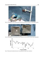
In our experiments, a commercial passive RFID system from Inside Contactless Inc. is used,
which consists of M300-2G RFID reader, circular loop antenna, and ISO 15693 13.56 MHz
coin type tags. Fig. 10 shows our experimental RFID based localization system, in which the
reader and the antenna are placed, respectively, on the top and at the bottom of a circular
shaped mobile robot. The antenna is installed at the height of 1.5 cm from the floor, and the
effective sensing radius is found to be about 10 cm through experiment. For experimental
flexibility, each tag is given a unique identification number, which can be readily mapped to
the absolute positional information.


Fig. 10. The experimental RFID based localization system
As a mobile robot navigates over the floor covered with tags, the antenna reads the
positional information from the tag within the sensing region, which is then sent to the
reader through the coaxial cable. The reader transmits the positional data to the notebook
computer at the rate of 115200 bps through RS-232 serial cable. Using a sequence of received
data, the notebook computer executes the embedded mobile robot localization algorithm
described in this paper.
To demonstrate the validity and performance of our RFID based mobile robot localization,
extensive test drives were performed. First, Fig. 11 shows the pseudorandom tag
arrangement on the floor that is used in our experiments. For easy installation, each four
tags having 10 cm sensing radius are attached on a 70
×70 cm square tile in a titled square
pattern. With different angles of rotation, given by (10), nine different square tiles are
constructed and their copies are made. Then, a total of sixteen square tiles are placed side
by side in a 4

×4 array, resulting in a 280×280 cm floor with the pseudorandom tag
Pseudorandom Tag Arrangement for Accurate RFID based Mobile Robot Localization

217
arrangement. At each test drive, a mobile robot is to travel along a right angled triangular
path shown in Fig. 11, where two perpendicular sides are set to be parallel to the x axis
and the y axis. A mobile robot is commanded at a constant speed of 10 cm/sec along three
linear segments, starting from (30,30), passing through (250,250) and (250,30), and
returning to (30,30).


Fig. 11. The experimental pseudorandom tag arrangement and the closed path trajectory


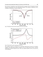
Fig. 12. The mobile robot velocity estimates: a) the forwarding speed and b) the steering
angle
Fig. 12 shows the componentwise plots of the estimated mobile robot velocities along the
right angled triangular path, obtained based on (4) and (6). Small difference between the
estimated and the actual mobile robot velocities can observed, which seem to be largely
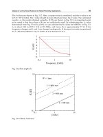
attributed to measurement noises involved. Next, Fig. 13 shows the componentwise plots of
the estimated mobile robot positions along the right angled triangular path, which are
computed from the mobile robot velocity estimates. The deviations from the actual mobile
Advanced Radio Frequency Identification Design and Applications

218
robot positions are also plotted in Fig. 13, which are again relatively small. Fig. 14 shows the
estimated and the actual mobile robot trajectories on the floor, marked by ‘x', and ‘o',
respectively. It can be observed that the estimated mobile robot trajectory is fairly close to
the actual one.

Fig. 13. The mobile robot localization: a) the componentwise positional estimates and b) the
deviations from the actual values


Fig. 14. The estimated trajectory, marked by ‘x', and the actual trajectory, marked by ‘o'
Pseudorandom Tag Arrangement for Accurate RFID based Mobile Robot Localization

219
Finally, the same test drive above was repeated 50 times to see how closely a mobile robot
can return to the starting position after the closed path navigation. Fig. 15 shows the plot of
the positional homing errors, which are the differences of the returning positions from the
starting position. It can be observed that the positional homing errors are kept less than 5
cm. Considering that the tag distribution density is relatively low, this result seems quite
satisfactory.


Fig. 15. The positional homing errors after the closed path navigations
6. Conclusion
This paper presented a pseudorandom RFID tag arrangement for improved performance of
mobile robot localization. First, using temporal as well as spatial information on tag
traversing, we developed a simple but effective mobile robot localization method. Second,
we examined four repetitive tag arrangements, including square, parallelogram, tilted
square, and equilateral triangle, in terms of tag installation and tag invisibility. Third, taking
into account both tag invisibility and tag installation, we proposed the pseudorandom tag
arrangement, inspired from the Sudoku puzzle. Currently, a study is under way for the
quantitative evaluation and optimal design of tag arrangements. We hope that the results of
this paper can provide an effective solution to the indoor localization of personal/service
robots.
7. Acknowledgement

This work was supported by the Hankuk University of Foreign Studies Research Fund of
2010, Republic of KOREA.
8. References
Borenstein, J., Everett, H. R., & Feng, L. (1996). Where am I? Sensors and Methods for Mobile
Robot Positioning, The University of Michigan
Advanced Radio Frequency Identification Design and Applications

220
Finkenzeller, K. (2000). RFID handbook: Fundamentals and Applications, Wiley.
Kubitz, O., Berger, M. O., Perlick, M. & Dumoulin, R. (1997). Application of radio frequency
identification devices to support navigation of autonomous mobile robots, Proc.
IEEE Vehicular Technology Conf., pp. 126-130
Kantor, G. & Singh, S. (2002). Preliminary results in read-only localization and mapping,
Proc. IEEE Int. Conf. Robotics and Automation, pp. 1818-1823
Hahnel, D., Burgard, W., Fox, D., Fishkin, K., & Philipose, M. (2004). Mapping and
localization with RFID technology, Proc. IEEE Int. Conf. Robotics and Automation,
pp. 1015-1020
Kulyukin, V, Gharpure, C., Nicholson, J. & Pavithran, S. (2004). RFID in robot-assisted
indoor navigation for the visually impaired, Proc. IEEE/RSJ Int. Conf. Intelligent
Robots and Systems, pp. 1979-1984
Penttila, K., Sydanheimo, L. & Kivikoski, M. (2004). Performance development of a high-
speed automatic object identification using passive RFID technology, Proc. IEEE
Int. Conf. Robotics and Automation, pp. 4864-4868
Yamano, K., Tanaka, K., Hirayama, M., Kondo, E., Kimura, Y., & Matsumoto, M. (2004).
Self-localization of mobile robots with RFID system by using support vector
machine, Proc. IEEE/RSJ Int. Conf. Intelligent Robots and Systems, pp. 3756-3761
Kim, B.K., Tomokuni, N., Ohara, K., Tanikawa, T., Ohba, K., & Hirai, S. (2006). Ubiquitous
localization and mapping for robots with ambient intelligence, Proc. IEEE/RSJ Int.
Conf. Intelligent Robots and Systems, pp. 4809-4814
Vorst, P., Schneegans, S., Yang, B., & Zell, A. (2008). Self-localization with RFID snapshots in

densely tagged environments, Proc. IEEE/RSJ Int. Conf. Intelligent Robots and
Systems, pp. 1353-1358
Bohn, J. and Mattern, F. (2004). Super-distributed RFID tag infrastructure, Lecture Notes in
Computer Science, vol. 3295, pp. 1-12
Choi, J., Oh, D., & Kim, S. (2006). CPR Localization Using the RFID Tag-Floor, Lecture Notes
in Computer Science, vol. 4099, pp. 870-874
Han, S., Lim, H., & Lee, J. (2007). An Efficient Localization Scheme for a Differential-Driving
Mobile Robot Based on RFID System, IEEE Trans. Industrial Electronics, vol. 54, no.
6, pp. 3362-3369
Kodaka, K., Niwa, H., Sakamoto, Y., Otake, M., Kanemori, Y., & Sugano, S. (2008). Pose
estimation of a mobile robot on a lattice of RFID tags, Proc. IEEE/RSJ Int. Conf.
Intelligent Robots and Systems, pp. 1385-1390
12
RFID Tags to Aid Detection of
Buried Unexploded Ordnance
Keith Shubert and Richard Davis
Battelle Memorial Institute
United States
1. Introduction
Detecting buried unexploded ordnance (UXO) at military firing ranges and elsewhere is
very difficult and expensive. To enable the military to conduct cost-effective training and
research missions in the future, with increased safety for personnel and property without
negative environmental impact, significant advances in detection and identification of
buried UXO must be pursued and implemented.
This chapter presents the results of analytical and experimental efforts that demonstrated
the viability of using munition-mounted radio frequency identification (RFID) tags as buried
ordnance detection and identification aids. RFID tagging of ordnance can provide a high
probability of detection and a near-zero false alarm rate. The tag provides discrimination
between UXO and clutter items, a capability that is critical to reducing the cost of UXO
remediation. This work was pursued because state-of-the-art passive RFID tags can

potentially provide information on the munitions’ locations while maintaining compatibility
with operational deployment. To ensure success, however, detection range below the
ground had to be investigated quantitatively.
The analysis was performed in the context of a UXO searching process that included the
movement of the transmit and receive coils in pre-defined lanes across a large land parcel.
The term “overlap” refers to the amount of overlap in two adjacent search lanes, i.e., the
portion of area retraced by the coil. This planned movement of the interrogation system’s
transmit and receive coils will reduce the impact of isolated nulls or minima within the field
patterns at both the tag and receive coil locations.
The operational concept calls for fastening tags to the exterior of candidate ordnance item as
part of the manufacturing process. During the detection segment of the UXO remediation
process, the UXO interrogation module provides energy to the tag by emitting a large
magnetic field. The munition-mounted tag responds by emitting a low-level digital signal
that is sensed by receivers on the UXO interrogation module. This research focused on low-
frequency, passive (non-battery) RFID tags, a choice made early in the investigation.
Extensive modeling of the RFID tag on the metal munition was performed to aid in
understanding the tag mounting parameters. The critical mounting concern is the required
separation between the tag and the metal of the munition because the customer required
detection of munitions buried as deep as one meter. For safety reasons, the transmitting coil
and RFID tag must be shown not to induce a large electric field near the munition because
too large a field might cause the munition to detonate.
Advanced Radio Frequency Identification Design and Applications

222
2. Background
Various methods for detecting buried unexploded ordnance at military firing ranges have
been investigated (GAO, 2004), (Halman, et al., 1998). These techniques involve scattering
energy off the munition and resolving the modified signal. Unfortunately, achieving
consistent results using these methods has proved to be difficult and expensive. The
techniques have also resulted in an unacceptable number of false-positive indications that

will significantly increase the cost of remediation because of the expense of excavating non-
UXO items. Using RFID tags, false alarms can occur only when a munition explodes and the
RFID tag survives. This event is thought to have such a low likelihood of occurring that a
statistical investigation of this scenario was not performed.
The method examined here differs from previous methods in that detection of the munition
is based on the energy received from a transmitting RFID tag affixed to the munition, as
depicted in Figure 1. The detection signal does not result from energy scattered by the
munition itself.


Fig. 1. Depiction of the tagged munition technique.
The ordnance detection system comprises an interrogation module and the RFID tag. The
above-ground interrogation module, used to search for tags, generates a large magnetic
field. The tag harvests the transmitted energy to power its integrated circuit and replies with
a digital signal. The interrogation module’s receive coil senses the digital signal transmitted
by the tag, then reports detection and any embedded digital data, which might include
information such as the munition type, serial number, and date of manufacture. One meter
deep detection of UXO was deemed necessary to demonstrate feasibility.
After determining which passive RFID tags offer the highest probability of success in this
application, additional electromagnetic and mechanical constraints were analyzed.
Electromagnetic considerations involved characterization of the ability to energize and
receive the reply from a passive RFID tag one meter from the excitation coil, the effect of the
presence of the munition’s metal on tag functionality, and the danger of the high-energy
transmitting coil setting off buried munitions. Mechanical considerations involved finding
ways to mount the RFID tags on existing metal munitions that allow RFID tag survival and
functionality, subject to the extreme accelerations associated with munitions and ordnance.
RFID Tags to Aid Detection of Buried Unexploded Ordnance

223
3. System design

3.1 RFID tag choice
According to Faraday’s and Lenz’ Law, the eddy currents induced on a conductive
munition will tend to oppose the magnetic field perpendicular to its surface. This opposition
becomes greater nearer the munition’s surface. Therefore, magnetic fields very near the
munition will tend to be parallel to its surface. This condition suggests choosing a
solenoidal-shaped tag mounted with its core parallel to the surface, allowing the most
efficient harvesting of energy from the interrogation module’s magnetic field.
One candidate solenoidal tag was the Texas Instruments (TI) Tiris RFID tags. The decision
was made to exploit these tags because of their operating frequency near 130 kHz and their
reliance on the magnetic field, both of which were favorable for maximum ground
penetration of the transmitted energy. Figure 2 shows the Texas Instruments’ Tiris solenoid
tags employed during this study on the left and the in the larger “pancake” geometry on the
right. The solenoid tags comprise a copper coil wrapped around a ferrite core, other circuit
elements, and a digitally-based integrated circuit that functions as a receiver, transmitter,
and processor with 64 bits of user-written data. The tags and readers employ frequency-shift
keying (FSK) between 123 kHz and 134 kHz to transmit the tag’s data to the reader.


Fig. 2. Two examples of the low-frequency passive tags. The photo on the left shows the
solenoid tag design; the coil wire is wrapped around a small permeable core. The photo on
the right shows the “pancake” coil design used in non-contact facility access applications.
The small black objects in the figures are the integrated circuits.
The RFID system choice was influenced by the Tiris tag’s response mechanism being more
favorable in this application. The Tiris tags do not reply until after the interrogation
module’s transmitter has turned off, which allows detection of the weak tag signal in a
quieter spectral environment. Alternative RFID systems have tags that reply during reader
interrogation, generally at half the reader’s transmitted frequency. This simultaneous
transmit and receive process in non-Tiris systems forces their readers’ detection systems to
detect very small signals in the presence of very large signals. Although this detection can
be accomplished, it requires very precise relative positioning of the transmitting and

receiving coils to minimize the magnitude of the transmitted signal cross-coupled into the
receiving coil. It was anticipated that maintaining the relative positions of the coils precisely
would be very difficult while traversing artillery and bomb ranges. The required positioning
accuracy is much less for the Tiris system because the transmitter is turned off while the
receiver is enabled.
Advanced Radio Frequency Identification Design and Applications

224
3.2 The transmit coil
The passive Tiris tags used in this study were intended to function with a separation
between the reader and the tag of about one meter under certain conditions. Because
budgetary constraints required that no changes be made to the RFID tags themselves, the
interrogation module would have to be modified and made larger to achieve the required
separation of one meter in the presence of the metal munition. The basic magnetic field
equations were examined to determine the possible ways to increase the field levels at
longer ranges. The magnetic field emitted in the z-direction, Bz, by a circular loop of radius a
in the x-y plane at a point located a distance r from the origin can be expressed in µW/m
2
as

2
0
3
22
2
2( )
z
INa
B
ar

μ
=
+
(1)
This relationship simplifies when the point r is located far from the coil as

2
0
3
1
()
2
z
INa
Bforra
r
μ
=
>> (2)
Equation (1) holds in regions near the coil, where the reduction as a function of r is slightly
less than 1/r
3
. The magnetic field increases linearly with the area of the coil, with the
current, and with the number of turns. For a given value of r (one meter) and a given value
of area (radius of one-half meter to keep the interrogating module from being too large), it
appears that one can arbitrarily increase B by either increasing the number of turns, N, or
the current, I. Practical considerations will limit the amount of current that can be employed
but it still appears that arbitrary increases in the number of turns will yield increasingly
large values of the magnetic field. Unfortunately, increasing the number of turns increases
the inductance of the coil. The value of the inductance can be seen in equations (3) and (4) to

increase as the square of the number of turns. The voltage across the coil is proportional to
the inductance as seen in equation (5). This relationship implies that the voltage is
proportional to N squared. Thus, for a given coil current, an arbitrary increase in N can
quickly drive the voltage across the coil to impractical values. An optimum combination of
N and I must be determined given the amount of current the batteries and drive circuit can
provide and the maximum tolerable voltage across the coil.

2
0.31( )
6910
aN
L
ah b
=
++
(3)

2
0.31
,
6
aN
Lforahb
=>>
(4)

dI
VL
dt
=

(5)
The final interrogation coil design included a diameter of one meter and Litz wire with
270 strands of 38 American wire gauge (AWG) magnet wire. The coil design employed
10 turns of Litz wire (N=10) and approximately 16 amps-rms, for a magnetomotive force of
160 ampere-turns-rms. These design values were confirmed to be effective through
RFID Tags to Aid Detection of Buried Unexploded Ordnance

225
laboratory experimentation and electromagnetic modeling of the interrogation system and
munition-mounted tag. No analytical optimization was attempted.
The laboratory investigation provided insight into potential detection ranges but it did not
answer the basic physics question of whether or not the tag mounted on or near a metallic
munition could function as needed.
3.3 Modeling approach
Knowledge of the magnetic field’s behavior is essential in understanding the overall system
designs required to transmit energy from the above-ground interrogator to the tag and from
the tag back to the above-ground receiver. Quantities of interest, such as signal strength, can
be calculated from these fields.
In the absence of the munition, the tag system’s general behavior is well known. However,
the tag’s necessarily close proximity to the metallic munition will affect its operation. These
passive tags are activated when there is sufficient magnetic energy linking its circuit’s pick-
up coil. Getting the requisite level of magnetic field to the tag for activation will be impeded
by the munition. Once activated, the tags generate a transmitted field that is altered by the
presence of the metal munition also.
Furthermore, the operational circuitry of the tag requires a specific quality factor (Q) to
operate (Shubert, 2007, 2008). The Q-value depends on the inductance and resistance of the
tag’s pick-up coil. These values will be distorted in the presence of the munition. If the Q-
value for the tag is too low, the tag cannot operate. There are of course other electromagnetic
factors interfering with the tag’s operation, but proximity to the munition is primary.
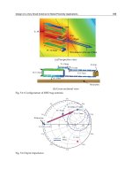
Figure 1 shows the basic geometry of the system as it was modeled. A transmitting coil

sends out a signal. If a tagged munition is within its range, the tag is activated and sends out
its own signal. The tag’s output signal is picked-up by a receiving coil.
For purposes of the modeling investigation, this basic system was decoupled into two
separate cases; (1) transmitting a signal to the tag and (2) receiving a signal from the tag.
These two cases are independent because the amplitude of the signal received by the
munition-mounted tag and the amplitude of the field transmitted by the tag are not related.
In both cases, the electric field was examined for Hazards of EM Radiation to Ordnance
(HERO) issues (Davis et al., 2006). The changes in Q-value of a tag were also examined
separately.
3.4 Magnetic modeling
The models consisted of two- and three-dimensional finite element models. For this task, the
commercially available finite element software package, Vector Fields, was used. Battelle
has successfully employed this type of modeling in other studies. Those results were
validated in both laboratory and field experiments.
Because the practical range of frequencies that will be used are on the order of a 100 kHz
and because the system antennas are in the near field, the models were solved using the
low-frequency Maxwell’s equations. For the two-dimensional models, equation (6) was
solved subject to appropriate boundary conditions. Here, A is the magnetic vector potential,
J
s
is the source current density,
σ
is the conductivity, and µ is the magnetic permeability.

1
()
S
A
AJ
t

σ
μ
∂
∇× ∇× = −
∂
(6)
Advanced Radio Frequency Identification Design and Applications

226
The curl of the vector potential, A, yields the magnetic field, B and its negative partial time
derivative yields the electric field, E. These two-dimensional models were used to provide
quick qualitative insights into the basic behavior of this system.
Although more time consuming, the three-dimensional models provided more useful
quantitative information. Equation (6) was used in the conductive regions and regions near
conductive materials. In all other regions, the magnetic scalar potential shown in
equation (7) was solved. Here, Φ
m
is the magnetic scalar potential. The solutions are
matched at the interfaces and are subject to appropriate boundary conditions. The gradient
of the magnetic scalar potential, Φ
m
, yields the magnetic field, B.

2
0
m
Φ
∇
=
(7)

Rather than employ an open-boundary technique, the mesh was extended to a reasonable
distance, a minimum of five times the distance between the munition and the transmit coil,
with a scalar potential boundary condition applied to the outer surface. This method
ensures that truncation has an insignificant effect on the region of interest. Although
requiring larger model sizes than the open-boundary technique, past experience indicates
that it provides a more accurate solution. The effect of truncation was estimated by
calculating the tangential component of the field on an open boundary with a derivative
boundary condition. Here, one-half the field observed on such a boundary is being reflected
back from the exterior. Combining this value with knowledge of the probable decay in the
exterior space gave an order of magnitude for the effect of the truncation on the regions of
interest. The effect of truncation was less than one part in a hundred.
In general, the two-dimensional models consisted of about 100,000 elements and had an
error relative to element size less than 0.25 percent. The three-dimensional models consisted
of about 800,000 elements and had an error relative to element size less than 1.0 percent.
Figure 3 shows an example of the basic three-dimensional models used for these
calculations including the cylindrical munition, a solenoid tag mounted on the munition,
and the transmit coil. The soil and air are not shown, but their interface is located along the
transmit coil’s plane.
For calculating the fields from the transmitting coils and tags, a uniform and constant source
current of 1 amp-turn was defined. The individual turns of transmitting coil wires need not
be modeled, provided the individual wire size is small compared to the coil diameter and
wavelength. Note that the source input is defined in terms of a constant current and not
voltage. The relationship between voltage and current input depends on the circuitry used
to drive the coils and is not important in modeling the fields.
Practically, the magnetic field levels generated will be such that the magnetic permeability
of all likely materials is constant. Therefore, the electromagnetic field results, upon which all
quantities of interest are calculated, will be linear with the number of amp-turns defined.
The calculated results can then be scaled for any strength transmitting coil or tag.
Once field levels are determined, signals to and from the tags can be calculated using
equation (8). Here

S is the signal strength, N is the number of turns in the receiving coil, B is
the magnetic field linking the receiving coil, and
a is the area of the coil. If a sinusoidal
waveform is assumed, the right hand side of equation (8) is obtained. Here
u
eff
is the
effective permeability of a receiving coil’s permeable core,
ω is the angular frequency, and B
o

is the calculated magnetic field linking the circuit in the absence of core permeability.
RFID Tags to Aid Detection of Buried Unexploded Ordnance

227

eff o
Coil
dB
SN daN Ba
dt
μ
ω
=⋅=
∫
G
G
(8)
The Texas Instruments tags specify a minimum
Q to respond to an interrogating signal.

Models of the tags near the munitions were used to calculate the changes in the
Q-value due
to their proximity to the metallic munition (Skilling, 1957).
Q can be defined in several ways
but two definitions stand out in this application. It is useful to define it as proportional to
the ratio of the inductance to the resistance of the tag’s receiving coil. It can also be defined
as the ratio of the resonance frequency to the bandwidth, which is a measure of the relative
narrowness of the resonance curve.


Transmitting Coil
Munition
Tag
Transmitting Coil
Munition
Tag

Fig. 3. The basic models for the munition, solenoid tag, and transmitting coil. The bottom
left figure shows the transmitting coil and munition. Here the coil is centered directly over
the munition and the ground is not shown. The other figures show the geometry (top-left
and bottom-right) and mesh (top-right) for the munition model. The tag is also shown
centered on the top surface of the model.
The resistance, R
c
, of the tag in free space is known a priori. Using the value of the
inductance, L, and resistance, R, caused by the nearby munition, the
Q-value is defined as

cQL/(RR)
ω

=
+ (9)
The value of
Q is dimensionless. The L and R values can be calculated from the
electromagnetic fields. The value of R is related to the power loss of the tag caused by
induced eddy current density,
J, in the munition. If I is the constant source current, the value
of R is given by

2
2
1
R
volume
J
dV
I
σ
=
∫
(10)
Advanced Radio Frequency Identification Design and Applications

228
The value of L is related to the magnetic energy created by the tag for a constant source
current. If B is the magnetic field as a function of space, the value of L is given by

2
2
1

volume
LBdV
I
μ
=
∫
(11)
The integrals are over all space containing conductive and/or permeable material.
The following parameters were examined to provide insight into the system with the intent
of proving feasibility and optimizing the system. These parameters were studied for all
three situations modeled using both two- and three-dimensional models. The parameters
being varied included:
•
Above-ground transmitter and receive coil positions relative to the munition
•
Soil type and conductivity (dry dirt to salt water)
•
Effect of nearby metallic or permeable materials
•
Munition depth
•
Munition orientation
•
Munition shape
•
Munition material
•
Tag type (solenoid or pancake)
•

Tag position on munition
•
Tag orientation
•
Tag mounting options such as tag offset from and “grooves” on the munition
•
Frequency of operation (both transmitter and tag)
For each situation, a baseline model was defined. These parameters were varied relative to
this baseline model to determine their effects.
3.4.1 Models for transmitting the signal from the tag
The fields at the munition surface near the above-ground receiving coil are critical to
understanding behavior. The flux from the tag linking the receiving coil’s windings will
determine whether the tag’s output signal can be detected.
The same basic munition geometry defined in the signal-to-the-tag case was used. The
effects of the transmit coil were ignored. A specific tag was modeled as being fastened to the
munition. Its location was variable. Both types of tags were modeled for baseline. Baseline
was a tag centered on the top of the munition with the same offset.
A receive coil does not need to be specifically modeled. The signal received from the tag by
a receive coil depends only on the magnetic field linking the receiver’s coil windings. This
value can be calculated independently using equation (8) once the model is solved.
3.4.2 Models for estimating effects on Q-values
Examination of the tags’ changes in Q-value due to the proximity of metallic munition was
done using two- and three-dimensional modeling. The model’s field output was calibrated
to commercial tags. Effects of various mounting techniques including separation (lift-off)
from the metallic surface were examined. The electromagnetic fields solved for these cases
were used to calculate the Q-value through the inductance and resistance using
equations (9) through (11).