Advances in Vibration Analysis Research Part 14 ppt
Bạn đang xem bản rút gọn của tài liệu. Xem và tải ngay bản đầy đủ của tài liệu tại đây (1.07 MB, 30 trang )
Vibration Analysis of a Moving Probe with Long Cable for Defect Detection of Helical Tubes
379
Fig. 10. Concept of the TICM: (a) connections of jth beam element and node j. (b) After the
connection of jth beam element, and (c) after the following connection of node j.
This is the concept of the TICM. A structure after the connection of jth beam element, and
following connection of node j are illustrated in Fig. 10(b and c), respectively. In the
formulation of the TICM for a step-by-step time integration, a relationship between the
displacement vector ( )
j
i
td and the force vector ()
j
i
t
f
illustrated in Fig. 10(b), before the
connection of node j, is defined as follows:
=+() () () ()
j
i
j
i
j
i
j
i
ttttdTfs (19)
We call the 3×3 square matrix
()
j
i
tT and three-dimensional vector ()
j
i
ts a dynamic influence
coefficient matrix and an additional vector of the left-hand side of node j, respectively. The
additional vector
()
j
i
ts represents an influence of external forces, which act on the preceding
nodes 0 to j−1, to displacement vector at node j.
Similarly, a relationship between
d
j
(t
i
) and f
j
(t
i
) illustrated in Fig. 10(c), after the connection
of node j, is defined as:
=+() () () ()
j
i
j
i
j
i
j
i
ttttdTfs (20)
where the matrix
T
j
(t
i
) and the vector s
j
(t
i
) are called a dynamic influence coefficient matrix
and an additional vector of the right-hand side of node j, respectively. The additional vector
s
j
(t
i
) represents an influence of external forces, which act on the preceding nodes 0 to j−1 and
newly connected node j.
In the algorithm of the TICM, the matrices
()
j
i
tT
, T
j
(t
i
) and vectors ()
j
i
ts , s
j
(t
i
) are
successively computed from node 0 (root of the probe) to node n (top of the probe) at first.
Subsequently, the displacement vectors are computed in the reverse order from node n to
node 0. Substituting Eq. (20) with subscript j−1 and Eq. (6) into Eq. (18) yields
−
−−−−
⎡
⎤
=+
⎢⎥
⎣⎦
+
++ −
+
T
1
TT
1,11,1
1
() () () ()
1
() [ ( ) ( )]
1
ji j j i jji j ji
v
jji jvji vji
v
ttt t
δB
δ
ttt
δB
dLTLf Ff
Ls Lh h
(21)
Comparing Eq. (21) with Eq. (19), we have
−
=+
+
1
1
() ()
1
t
j
i
jj
i
jj
v
tt
δB
TLTL F (22a)
Advances in Vibration Analysis Research
380
−−−−
=+ −
+
1,11,1
() () [ ( ) ( )]
1
tt
ji jj i jvj i vji
v
δ
tt tt
δB
sLs Lh h
(22b)
Multiplying both sides of Eq. (17) by
()
j
i
tT and utilizing the relationship () ()
j
i
j
i
ttT
f
= d
j
(t
i
) −
()
j
i
ts [Eq. (19)] yields
−−
+=++
31 1
[ () ( )] () () () () () ( )
ji ji ji ji ji ji ji ji
tt t tt t ttIT P d T f s T q (23)
Comparing Eq. (23) with Eq. (20), we obtain
−
+=
31
[ () ( )] () ()
j
i
j
i
j
i
j
i
tt t tIT P T T
(24a)
31 1
[ () ( )] () () () ( )
ji ji ji ji ji ji
tt t t tt
−−
+=+IT P s s T q (24b)
where
I
3
is a 3×3 unit matrix. We call Eqs. (22a), (22b) and (24a), (24b) “field transmission
rule” and “point transmission rule”, respectively. Supposing that the dynamic influence
coefficient matrix and additional vector of the right-hand side of node j−1,
T
j−1
(t
i
) and s
j−1
(t
i
),
are known, the ones of node j, that is
T
j
(t
i
) and s
j
(t
i
), are obtained through the field and point
transmission rules Eqs. (22a), (22b) and (24a), (24b). In other words, if the dynamic influence
coefficient matrix and additional vector of node 0 are known, the ones of other nodes are
successively computed from node 1 to node n because the field and point transmission rules
represent a recurrent formula to yield
T
j
(t
i
) and s
j
(t
i
). Since the root of the probe, node 0, is
assumed to have no relative movement with respect to the unstretched probe, the
displacement and force vectors at node 0 are regarded as
d
0
(t
i
) = 0 and f
0
(t
i
) ≠ 0. Substituting
the
d
0
(t
i
) and the f
0
(t
i
) into Eq. (20) with subscript j
=
0, we obtain the dynamic influence
coefficient matrix and additional vector of node 0.
030
() , ()
ii
tt==Ts00 (25)
where
0
3
is a 3×3 zero matrix.
Node j slantingly connects with the jth and (j+1)th beam elements as shown in Fig. 7.
Therefore, coordinate transform is necessary through the point transmission rule. The
transform of coordinate from jth beam element to node j is operated as:
T
cos sin 0
() (), () (), sin cos 0
001
ji ji ji ji
φφ
tttt φφ
−
⎡
⎤
⎢
⎥
⇒⇒=
⎢
⎥
⎢
⎥
⎣
⎦
ΦT Φ T Φ ssΦ
(26a)
The transform of coordinate from node j to (j+1)th beam element is operated as:
T
() (), () ()
j
i
j
i
j
i
j
i
tttt⇒⇒ΦT Φ T Φ ss
(26b)
The dynamic influence coefficient matrix T
j
(t
i
) and additional vector s
j
(t
i
) are successively
computed from node 0 to node n through Eqs. (22a), (22b), (24a)–(26b).
The right-hand side of the system (top of the probe) is free, it follows that the force vector at
the right-hand side of node n is zero, that is f
n
(t
i
) = 0. Substituting f
n
(t
i
) = 0 into Eq. (20), we
obtain the displacement vector of node n as:
() ()
ni ni
tt=ds (27)
Vibration Analysis of a Moving Probe with Long Cable for Defect Detection of Helical Tubes
381
Displacement vectors of other nodes are recursively obtained from node n−1 to node 0 by
applying the following equations, which are derived from Eqs. (17), (6) and (20).
111
1111
() ( ) () ( ) (), () ()
() () () ()
j
i
j
i
j
i
j
i
j
i
j
i
jj
i
ji jiji ji
tt ttt t t
tttt
−−−
−−−−
=+− =
=+
fq fPd f Lf
dTfs
(28)
where j : n
→ 1. The following coordinate transform is also necessary for ()
j
i
t
f
and f
j−1
(t
i
) in
the process of Eq. (28) because of the slanting connection of jth beam element with node j−1
and node j.
TT
11
() (), () ()
j
i
j
i
j
i
j
i
tt t t
−−
⇒⇒Φ ffΦ ff (29)
Velocity and acceleration vectors
()
j
i
td
and
()
j
i
td
are given by Eq. (16) after the
computation of displacement vectors d
j
(t
i
).
4. Numerical computations
4.1 Reproduction of the experimental results
Numerical simulations were implemented by using the analytical model obtained in Section
2. A standard computer (CPU 2.4 GHz, 512MB RAM) was used in the computation. The
compiler was Fortran 95 and double precision variables were used. The Newmark-β method
(β
=
1/4, γ
=
1/2) was employed as a step-by-step time integration scheme. We confirmed
Table 2. Parameters of numerical simulation
that the results by the Wilson-θ method (θ
=
1.4) were almost the same as the ones by the
Newmark-β method.
Parameters of the numerical simulation are listed in Table 2. Since probes of constant length
are treated, five probes with different length are provided for numerical simulation. The five
Advances in Vibration Analysis Research
382
probes are different in length of carrier cable, l
=
10, 20, 30, 40 and 50m as listed in Table 2.
The total length of the cable L is the length of carrier cable l plus that of guide cable l
G
=
2.5
m. As mentioned in Section 2.2 (b), numerical simulation of the probe is approximately
regarded as a momentary situation in which the inserted length of the probe into the helical
part of the heating tube reaches L. An initial condition was assumed to be static. The drag
force of Eq. (10) simultaneously began to act on the all floats at the beginning of the
simulation. At the same time, the probe began to move at a feeding speed u. Time step size
∆t
=
0.0001 s was chosen for the step-by-step integration and time historical responses
during t
=
0
–
8 s were computed. The numerical simulations were impossible because of a
numerical divergence when the time step size was larger than 0.0001 s in both the
Newmark-β and the Wilson-θ methods.
Displacements of the node corresponding to the sensor are shown in Fig. 11. Axial
displacement x
j
(t) and radial displacement y
j
(t) are shown in Fig. 11(a and b), respectively.
The vibration of the probe increases as the length of probe become longer. Particularly, the
radial displacement rapidly increases between l
=
30 and 40 m. Since the vibration of probe
in experiment rapidly increased after the sensor passed through the middle point of the
helical part (see Fig. 4), the results of the numerical simulation agree with the experimental
results.
Fig. 11. Vibration of probe in insertion process: (a) axial and (b) radial displacements.
Finally, the inserted length of the probe into the helical heating tube reaches 55–60 m.
Magnifications of the axial and the radial vibrations of l
=
55 m (total length L
=
l
+
l
G
(2.5m)
=
57.5
m) are shown in Fig. 12(a and b). Other parameters were the same as the ones listed in
Table 2. The vibrations during t
=
1.0–2.5 s are plotted. It is confirmed that the axial and the
Vibration Analysis of a Moving Probe with Long Cable for Defect Detection of Helical Tubes
383
radial vibrations are weakly coupled. The locus of the vibration is plotted in Fig. 13(a). The
horizontal axis indicates a fixed coordinate along the inner wall of the heating tube and the
vertical axis shows the radial displacement. The probe is leaping around and shows an
inchworm-like motion. The motion of the sensor in the experiment, where the inserted
length of the probe into the helical part was about 57 m, is shown in Fig. 13(b). It was given
by a tracing of the images of sensor, which was taken by a high-speed camera. Although
both the axial and the radial motions in the experiment are larger than that of the
simulation, the result of the simulation qualitatively agrees with the one of the experiment.
The Fourier analysis of the axial and the radial vibrations of L
=
57.5 m are shown in Fig.
14(a and b), respectively. The vibrations during t
=
0.5–4.5 s, which are free from the
transient response, are provided to the Fourier analysis. It is confirmed that the axial and the
radial vibrations are coupled since an identical peak of 14 Hz appears in both vibrations.
The frequency of the coupled vibration in the experiment was about 20 Hz, as mentioned in
Section 2.1 c. There is a discrepancy between the experiment and the numerical simulation
in this point. However, the results of numerical simulations are qualitatively similar to the
ones of the experiment.
Fig. 12. Vibration of probe; l
=
55
m, t
=
1.0–2.5 s: (a) axial and (b) radial displacements.
Fig. 13. Locus of probe; (a) numerical simulation of l=55
m, t=1.8–2.2 s and (b) in experiment,
inserted length around 57
m.
Fig. 14. Frequency analysis of vibration; l
=
55m : (a) axial and (b) radial displacements.
Advances in Vibration Analysis Research
384
A numerical simulation of the probe without feeding (feeding speed u
=
0 mm/s) was
implemented. The length of carrier cable was l
=
50 m, which showed a severe vibration with
feeding speed u
=
200 mm/s as shown in Fig. 11. Other parameters were the same as the
ones listed in Table 2. This simulation corresponds to the experiment that the dry
compressed air streamed in the heating tube but the probe was not fed as mentioned in
Section 2.1 d. Displacements of the node corresponding to the sensor are shown in Fig. 15.
Both the axial and the radial displacements converged at constant values after an initial
transient response. This result is similar to the experiment. It follows that the experimental
result without feeding is also supported by the numerical simulation.
Fig. 15. Response at u
=
0 mm/s; l
=
50m : (a) axial and (b) radial displacements.
More numerical simulations were implemented in order to enhance the validity of the
analytical model. Numerical simulations with variation of feeding speed, diameter of the
helix and air supply rate were implemented. Only one parameter (feeding speed, diameter
of the helix or air supply rate) was changed, and the other parameters were the same as
Table 2. The length of carrier cable was l
=
50 m as well as the simulation of the non-feeding
probe, Fig. 15. The simulations of feeding speed u
=
100 and 400 mm/s, diameter of the helix
d
h
=
2.5 m and air supply rate Q
=
40m
3
/h are shown in Figs. 16–18, respectively. In Fig.
16,the vibration of the probe became small at low feeding speed u = 100 mm/s, but large at
high feeding speed u
=
400 mm/s, compared with the result of l
=
50 m in Fig. 11 (u
=
200
mm/s). The vibration also became small in the case of large helical diameter (Fig. 17) and
low supply rate of the air flow (Fig. 18). These results are similar to the experiments
mentioned in Section 2.1 f. Note that in the case of Q
=
40m
3
/h, an ability to insert the actual
probe is not guaranteed for lack of a drag force (Inoue et al., 2007).
Fig. 16. Vibration of probe; l
=
50m: (a) axial and (b) radial displacements at feeding speed
u
=
100 mm/s, (c) axial and (d) radial displacements at u
=
400 mm/s.
Vibration Analysis of a Moving Probe with Long Cable for Defect Detection of Helical Tubes
385
Fig. 17. Vibration of probe; diameter of helix d
h
= 2.5 m, l = 50m: (a) axial and (b) radial
displacements.
Fig. 18. Vibration of probe; air supply rate Q
=
40
m
3
/h, l
=
50
m: (a) axial and (b) radial
displacements.
The numerical simulation was qualitatively able to reproduce the experimental results.
Thus, the validity of the analytical model obtained in this study was confirmed through the
numerical simulations. It was demonstrated that the vibration of probe was caused by
Coulomb friction between the floats and the inner wall of the heating tube.
4.2 Entire behavior of probe
A numerical simulation of the insertion process to the length of carrier cable l
=
55 m is
implemented, and the entire probe behavior is shown in Fig. 19. The other parameters are
the same as the ones in Table 2. The total length of the cable is L = l (55 m) + l
G
(2.5 m) = 57.5
m. Momentary shapes of the entire probe during 1.56–1.65 s are displayed at an interval of
0.01 s. Axial and radial displacements are shown in Fig. 19(a and b), respectively. Each of the
horizontal axes in Fig. 19(a and b) indicates a distance from the entrance of the helical
heating tube. It is a fixed coordinate along the helical heating tube. The root of the probe,
which is supposed to be located at the entrance of the helical heating tube, corresponds to L
=
0 m, and the top of the cable is situated at L
=
57.5 m. The vertical axes in Fig. 19(a) indicate
the axial displacements, and the ones in Fig. 19(b) indicate the radial displacements.
Although the direction of the axial displacement in the ordinate of Fig. 19(a) is the same as
the coordinate along the heating tube L, it is displayed at right angles with the coordinate L.
The sensor position is indicated as broken lines both in Fig. 19(a and b). The following
characteristics are found in Fig. 19.
a. A shaded area in Fig. 19(a) indicates a segment in which a gradient of the axial
displacement along the heating tube (dx/dL) obviously shows a negative value. The
identical areas are also shaded in Fig. 19(b). We are able to observe a radial
displacement in the shaded area. Furthermore, it becomes larger as the negative
gradient of the axial displacement (dx/dL < 0) becomes steeper.
b. Local maxima of the axial displacement, points “A” and “B” in Fig. 19(a), move toward
the top of the probe as the time step goes forward. This is a wave-like motion rather
than a vibration. A reflection of the wave is not clearly observed in Fig. 19(a and b). It
Advances in Vibration Analysis Research
386
seems that the noticeable peak at 14 Hz in Fig. 14 signifies the frequency of
repetitiveness of the wave-like motion.
Fig. 19. Entire behavior of probe in the insertion process: (a) axial and (b) radial displacements.
c. Large amplitudes in the radial displacement are limited in the area near the top of the
cable.
The countermeasures against vibration, which include a long guide cable and a large float of
guide cable, were devised in order to reduce the RF sensor noise. It was confirmed that the
countermeasures are effective in suppressing the vibration in the experiments. Although the
countermeasures were empirically obtained, the entire behavior of the probe shown in Fig.
19 implies the mechanism of the countermeasures as follows:
Vibration Analysis of a Moving Probe with Long Cable for Defect Detection of Helical Tubes
387
a. The amplitude in the radial displacement is small at a position away from the top of the
cable as shown in Fig. 19(b). The long guide cable keeps the sensor part away from the
top of the cable, and the radial (displacement) vibration at the sensor position becomes
small. Since the RF sensor noise is highly correlated to the radial vibration, it is reduced
by means of the long guide cable. This effect has been also confirmed in the
experiments (Inoue et al., 2007a).
b. In the shaded area in Fig. 19, where the gradient dx/dL<0, the driving force (drag force)
acting on the probe is smaller than that of the non-shaded area. Originally, a tensile
force acts on the probe in the insertion process. However, a “compressive force” is
generated in the shaded area because of the lack of driving force, and the shaded area is
pushed from the backward non-shaded area. Consequently, a kind of buckling happens
and the probe in the shaded area, which is supposed to move in contact with the inside
of the helical tube, rises off the inner wall of the heating tube. This phenomenon travels
toward the top of the cable and makes the wave-like motion. At a fixed point, for
example the sensor position, it appears as a vibration. This is the mechanism of the
probe vibration. Similar rising (lift-off) phenomena were reported in previous studies
(Bihan, 2002; Giguere et al., 2001; Tian and Sophian, 2005), but significant vibration was
not reported in these studies. Relatively severe vibration induced by this rising
phenomenon is a peculiar characteristic of this study. Since the shaded area is generated
in the forward section of the probe, the large float of guide cable makes the driving
force acting on the forward section large, and it reduces the “compressive force” acting
on the shaded area. As a result, the large float of guide cable works to suppress the
vibration at the sensor part.
4.3 Improvement of the countermeasure
The empirical countermeasures to suppress the vibration at the sensor part are supported by
the numerical simulations. On the basis of the mechanism which suppresses the vibration,
the following improvements are suggested:
a. Use of a longer guide cable. This acts on the principle that the vibration becomes
smaller as the length between the sensor position and the top of cable becomes longer.
b. Further increase of the driving force of the guide cable. This makes the “compressive
force” acting on the forward section of the probe relatively weak, and prevents the
probe from rising off the inner wall of the heating tube.
c. Decrease the driving force of the carrier cable. This is similar to suggestion b. It directly
reduces the “compressive force” toward the forward section of the probe by reducing
the driving force of the backward section.
In reference to suggestion a, it makes the probe length inserted into the heating tube longer.
Since the steam generator of the “Monju” has 140-layered heating tubes, use of an
excessively long guide cable would negatively affect maintenance efficiency. Thus, a guide
cable longer than 10m is undesirable in actual use. Suggestions b and c involve control of the
drag force acting on the floats. There are two means to vary the drag force: One is to alter
the float size, where the float is spherical. The other is to replace the float shape. However, it
is difficult to practicably use a non-spherical float as it would compromise the smooth
passage of the probe. Hence, control of the drag force by alteration of the float size is
considered here.
Advances in Vibration Analysis Research
388
The inner diameter of the heating tube is 24.2 mm, and some points are smaller than 24.2mm
because of projections caused by welding. Consequently, a float diameter of 20 mm, which
has been utilized in the countermeasure, seems to be the upper limit since a larger float
would probably clog the heating tube. Thus, only suggestion c is adopted. The probe is fed
into the upper side of the steam generator (see Fig. 1), goes down the heating tube, passes
the helical part, goes up the straight part and reaches the upper side again. A strong driving
force is needed when the probe passes the helical part and goes up the straight part of
heating tubes. Thus, there is also a minimum float diameter in order to guarantee the
driving force needed to propel the probe to achieve the inspection of the heating tubes. We
choose the diameter for the float attached to carrier cable d
f
=
16 mm.
The numerical simulation with these improvements, where the length of guide cable l
G
=
10
m, the diameter of the float attached to guide cable d
f
=
20 mm and the one to carrier cable d
f
=
16 mm, is implemented. The length of carrier cable l = 50 m, (total length L is 60 m) and the
other parameters are the same as the ones in Table 2. The vibration at the sensor part is
shown in Fig. 20. Suppression of the vibration at the sensor part is almost accomplished in
the radial direction. Comparing this result with the one of l
=
50 m in Fig. 11, the validity of
this improvement is indisputable. We can assess that the performance of the improved
probe is satisfactory to suppressing the vibration.
Fig. 20. Vibration of probe in the insertion process with the proposed improvement,
diameter of the float attached to the guide cable 20
mm, carrier cable 16mm and length of the
guide cable l
G
=
10
m : (a) axial and (b) radial displacements.
In 2010, the fast breeder reactor “Monju” in Japan resumed work after a long time tie-up of
operation. The tie-up was cause by a leakage accident of sodium in a heat exchanging
system. The resumption of “Monju” was the target of public attention. An improved probe
based on this study practically come into service for the defect detection of heating helical
tubes installed in “Monju”. A reliable inspection is performed and it has kept a safe
operation of “Monju”.
5. Conclusions
A defect detection of a helical heating tube installed in a fast breeder reactor “Monju” in
Japan is operated by a feeding of an eddy current testing probe. A problem that the eddy
current testing probe vibrates in the helical heating tubes happened and it makes the
detection of defect difficult. In this study, the cause of the vibration of the eddy current
testing probe was investigated. The results are summarized as follows:
a. The cause of the vibration was assumed to be Coulomb friction and an analytical model
of the vibration incorporating Coulomb friction was obtained.
b. An effectual algorithm for the numerical simulation of the eddy current testing probe
was formulated by applying the Transfer Influence Coefficient Method to the equation
of motion derived from the analytical model.
Vibration Analysis of a Moving Probe with Long Cable for Defect Detection of Helical Tubes
389
c. The results of numerical simulations qualitatively reproduced the several characteristics
of the vibration of the eddy current testing probe, which were obtained by experiments.
The validity of the assumption that the vibration is cause by Coulomb friction was
confirmed by an agreement between the results of experiments and numerical
simulations.
d. The probe’s motion in its entirety under the vibration conditions was obtained by the
numerical simulation. The mechanism of the vibration and the countermeasures were
revealed through a discussion on the probe’s entire motion.
e. An improvement of the countermeasure was proposed based on the probe’s entire
motion. The validity of the proposed improvement was demonstrated through a
numerical simulation. The improvement was effective both in the insertion and the
return processes.
6. Acknowledgements
This investigation was performed through collaboration between Kyushu University and
Japan Atomic Energy Agency (JAEA) as public research of Japan Nuclear Cycle. Here the
authors would like to acknowledge the authorities concerned.
7. References
Belytschko, T. & Hughes, T.J.R. (1983). Computational methods for transient analysis,
Belytschko, T. & Bathe, K.J. (Eds.), Computational Methods in Mechanics, Vol. 1,
(417–471), Elsevier Science Publishers B.V., ISBN 0444864792, Amsterdam.
Bihan, Y.L. (2002). Lift-off and tilt effects on eddy current sensor measurements: a 3-D finite
element study. Eur. Phys. J. Appl. Phys., Vol. 17, (25–28), ISSN 0021-8979.
Crisfield, M.A. & Shi, J. (1996). An energy conserving co-rotation procedure for non-linear
dynamics with finite elements. Nonlinear Dyn., Vol. 9, (37–52), ISSN 1090-0578.
Giguere, S.; Lepine, B. & Dubois, J.M.S. (2001). Pulsed eddy current technology:
characterizing material loss with gap and lift-off variations. Res. Nondestructive
Eval., Vol. 13, (119–129), ISSN 1075-4862.
Inoue, T.; Sueoka, A.; Nakano, Y.; Kanemoto, H.; Imai, Y. & Yamaguchi, T. (2007). Vibrations
of probe used for the defect detection of helical heating tubes in a fast breeder
reactor. Part 1. Experimental results by using mock-up. Nucl. Eng. Des., Vol. 237,
(858–867), ISSN 0029-5493.
Inoue, T.; Sueoka, A. & Shimokawa, Y. (1997). Time historical response analysis by applying
the Transfer Influence Coefficient Method, Proceedings of the Asia-Pacific Vibration
Conference ’97, Vol. 1, pp. 471–476, Kyongju (Korea), November 1997.
Isobe, M.; Iwata, R. & Nishikawa, M. (1995). High sensitive remote field eddy current testing by
using dual exciting coils, Collins, R.; Dover, W.D.; Bowler, J.R. & Miya, K. (Eds.),
Nondestructive Testing Mater. (Studies in Applied Electromagnetics and
Mechanics), Vol. 8, (145–152). IOS Press, ISBN 9051992394, Amsterdam.
Kondou, T.; Sueoka, A.; Moon, D.H.; Tamura, H. & Kawamura, T. (1989). Free vibration
analysis of a distributed flexural vibrational system by the Transfer Influence
Coefficient Method. Theor. Appl. Mech., Vol.37, (289–304), ISSN 0285-6024.
Pestel, E.C. & Leckie, F.A. (1963). Matrix Methods in Elastomechanics, McGraw-Hill
Publishers, ISBN 0070495203, New York.
Advances in Vibration Analysis Research
390
Robinson, D. (1998). Identification and sizing of defects in metallic pipes by remote field
eddy current inspection. Tunnel. Underground Space Technol, Vol. 13, (17–27), ISSN
0886-7798.
Sueoka, A.; Tamura, H.; Ayabe, T. & Kondou, T. (1985). A method of high speed structural
analysis using a personal computer. Bull. JSME, Vol. 28, (924–930), ISSN 1344-7653.
Tian, G.Y. & Sophian, A. (2005). Reduction of lift-off effects for pulsed eddy current NDT.
NDT&E Int., Vol. 38, (319–324), ISSN 0963-8695.
Xie, Y.M. (1996). An assessment of time integration schemes for non-linear dynamic
equations. J. Sound Vibrat., Vol. 192, (321–331), ISSN 0022-460X.
20
Vibration and Sensitivity Analysis of
Spatial Multibody Systems Based on
Constraint Topology Transformation
Wei Jiang, Xuedong Chen and Xin Luo
Huazhong University of Science and Technology
P.R.China
1. Introduction
Many kinds of mechanical systems are often modeled as spatial multibody systems, such as
robots, machine tools, automobiles and aircrafts. A multibody system typically consists of a
set of rigid bodies interconnected by kinematic constraints and force elements in spatial
configuration (Flores et al., 2008). Each flexible body can be further modeled as a set of rigid
bodies interconnected by kinematic constraints and force elements (Wittbrodt et al., 2006).
Dynamic modeling and vibration analysis based on multibody dynamics are essential to
design, optimization and control of these systems (Wittenburg, 2008 ; Schiehlen et al., 2006).
Vibration calculation of multibody systems is usually started by solving large-scale
nonlinear equations of motion combined with constraint equations (Laulusa & Bauchau,
2008), and then linearization is carried out to obtain a set of linearized differential-algebraic
equations (DAEs) or second-order ordinary differential equations (ODEs) (Cruz et al., 2007;
Minaker & Frise, 2005; Negrut & Ortiz, 2006; Pott et al., 2007; Roy & Kumar, 2005). This kind
of method is necessary for solving the dynamics of nonlinear systems with large
deformation.
However, there are two major disadvantages for vibration calculation of multibody systems
by using the conventional methods. On one hand, the computational efficiency is very low
due to a large amount of efforts usually required for computation of trigonometric
functions, derivation and linearization. Many approaches have been proposed to simplify
the formulation, such as proper selection of reference frames (Wasfy & Noor, 2003),
generalized coordinates (Attia, 2006; Liu et al., 2007; McPhee & Redmond, 2006; Valasek et
al., 2007), mechanics principles (Amirouche, 2006; Eberhard & Schiehlen, 2006), and other
methods
(Richard et al., 2007; Rui et al., 2008). On the other hand, despite sensitivity analysis
of multibody systems based on the conventional methods are well documented (Anderson &
Hsu, 2002; Choi et al., 2004; Ding et al., 2007; Sliva et al. 2010; Sohl & Bobrow, 2001; Van
Keulen et al. 2005; Xu et al., 2009), the formulation is quite complicated because the resulting
equations are implicit functions of the design parameters.
Actually, what people concern, for many kinds of mechanical systems under working
conditions, are eigenvalue problems and the relationship between the modal parameters
and the design parameters. And the designer needs to know the results as quickly as
possible so as to perform optimal design. From this point of view, fast algorithm for
Advances in Vibration Analysis Research
392
vibration calculation and sensitivity analysis with easiness of application is critical to the
design of a complex mechanical system. A novel formulation based on matrix
transformation for open-loop multibody systems has been proposed recently
(Jiang et al.,
2008a). The algorithm has been further improved to directly generate the open-loop
constraint matrix instead of matrix multiplication (Jiang et al., 2008b). The computational
efficiency has been significantly improved, and the resulting equations are explicit functions
of the design parameters that can be easily applied for sensitivity analysis. Particularly, the
proposed method can be used to directly obtain sensitivity of system matrices about design
parameters which are required to perform mode shape sensitivity analysis (Lee et al., 1999a;
1999b).
Vibration calculation of general multibody system containing closed-loop constraints is
investigated in this article. Vibration displacements of bodies are selected as generalized
coordinates. The translational and rotational displacements are integrated in spatial
notation. Linear transformation of vibration displacements between different points on the
same rigid body is derived. Absolute joint displacement is introduced to give mathematical
definition for ideal joint in a new form. Constraint equations written in this way can be
solved easily via the proposed linear transformation. A new formulation based on
constraint-topology transformation is proposed to generate oscillatory differential equations
for a general multibody system, by matrix generation and quadric transformation in three
steps:
1. Linearized ODEs in terms of absolute displacements are firstly derived by using
Lagrangian method for free multibody system without considering any constraint.
2. An open-loop constraint matrix
′
B is derived to formulate linearized ODEs via quadric
transformation
=
=
′′′
T
(,,)
E
BEB E MKC for open-loop multibody system, which is
obtained from closed-loop multibody system by using cut-joint method.
3. A constraint matrix
′
′
B
corresponding to all cut-joints is finally derived to formulate a
minimal set of ODEs via quadric transformation
=
=
′′ ′′ ′ ′′
T
(,,)
E
BEB E MKC for closed-
loop multibody system.
Complicated solving for constraints and linearization are unnecessary for the proposed
method, therefore the procedure of vibration calculation can be greatly simplified. In
addition, since the resulting equations are explicit functions of the design parameters, the
suggested method is particularly suitable for sensitivity analysis and optimization for large-
scale multibody system, which is very difficult to be achieved by using conventional
approaches.
Large-scale spatial multibody systems with chain, tree and closed-loop topologies are taken
as case studies to verify the proposed method. Comparisons with traditional approaches
show that the results of vibration calculation by using the proposed method are accurate
with improved computational efficiency. The proposed method has also been implemented
in dynamic analysis of a quadruped robot and a Stewart isolation platform.
2. Fundamentals of multibody dynamics
2.1 Description of multibody system
As shown in Fig. 1, considering a multibody system which consists of
n
rigid bodies and
the ground
0
B , each two bodies are probably interconnected by at most one joint and
arbitrary number of spatial spring-dampers. A spatial spring-damper means an integration
Vibration and Sensitivity Analysis of Spatial Multibody Systems
Based on Constraint Topology Transformation
393
of three spring-dampers and three torsional spring-dampers. Each joint contains at least one
and at most six holonomic constraints.
i
B denotes the
th
i rigid body, and
ij
J is the joint
between
i
B and
j
B , where
=
",1,2,,ij nand
≠
ij.
ij
s denotes the total number of spring-
dampers between
i
B and
j
B , among which
ijs
K is the
th
s one, where
=
"0,1,2, ,
ij
ss. = 0
ij
s
means there is no spring-damper between
i
B and
j
B .
Four kinds of reference frames are used in the formulation. The global reference frame,
namely the inertial frame, i.e., -o xyz , is fixed on the ground. The body reference frame, e.g.,
-
i
c xyz for
i
B , is fixed in the space with its origin coinciding with the center of mass (CM) of
the body. For simplicity without loss of generality, all body reference frames are set to be
parallel to -o xyz in this paper. The spring reference frame, e.g.,
′
′′
-
ijs
u xyz for
ijs
K , is located at
one of the spring acting points. The joint reference frame, e.g.,
′
′′′′′
-
ij
v xyz for
ij
J , is located at
one of the joint acting points.
Fig. 1. Elements and reference frames in multibody system
Define
i
m the mass of
i
B ,
i
J the inertia tensor of
i
B with respect to -
i
c xyz , and I the 3×3
identity matrix. Then the mass matrix of body
i
B with respect to -
i
c xyz is given by
=
dia
g
()
iii
m
M
IJ (1)
The mass matrix of the free multibody system can be organized as
= "
12
dia
g
()
n
MMMM
(2)
The translation of CM of
i
B
is specified via vector
=
T
[]
iiii
xyzr . The rotation of
i
B
is
specified via Bryan angles
α
βγ
=
T
[]
iiii
θ . The absolute angular velocities can be written as
(Wittenburg, 2008)
βγ γ
βγ γ
β
α
ω
ω
β
ω
γ
⎡
⎤
⎡⎤⎡ ⎤
⎢
⎥
⎢⎥⎢ ⎥
==−
⎢
⎥
⎢⎥⎢ ⎥
⎣⎦⎣ ⎦
⎣
⎦
0
0
01
i
ix i i i
iiy iii i
iz i i
CC S
CS C
S
ω
(3)
where
μ
μ
S=sin ,
μ
μ
μαβγ
=
=Ccos( ,,)
iii
.
Due to small angular displacements of bodies, i.e.,
α
βγ
≈
,, 0
iii
, the absolute angular
velocities and displacements can be linearized as (Wittenburg, 2008)
αβγ
≈
=
T
[]
iiii i
ωθ
(4)
Advances in Vibration Analysis Research
394
Θ
=≈=
∫∫
dd
iii
ttωθθ (5)
The spatial displacements of
i
B
can be unified as
α
βγ
=
=
TTT T
[][ ]
iii iiiiii
xyzqrθ (6)
The displacements and velocities for free multibody system can be organized as
= "
TT TT
12
[]
n
qqq q
and
=
"
TT TT
12
[]
n
qqq q
.
The stiffness and damping coefficients of
ijs
K
are defined in spring reference frame
′′′
-
ijs
u xyz
as
(
)
αβγ
= diag
u
ijs x y z
kkkkkkK ,
(
)
αβγ
= diag
u
ijs x y z
ccccccC .
ijs
P
and
jis
P
are the acting
points of
ijs
K
on
i
B and
j
B
.
=
T
[]
ijs ijs ijs ijs
xyzr
denotes the original position of
ijs
P
relative to
-
i
c xyz
.
=
T
[]
jis jis jis jis
xyzr
denotes the original position of
jis
P
relative to
-
j
cxyz
.
α
βγ
=
T
[]
ijs ijs ijs ijs
θ denotes the original orientation of
ijs
K
relative to
-
i
c xyz
.
Most of the joints that used for practical applications can be modeled in terms of the so-
called lower pairs, including revolute, prismatic, cylindrical, universal, spherical, and planar
joints. Each joint reduces corresponding number of degrees of freedom (DOFs) of the distal
body (Pott et al., 2007; Müller, 2004) between two connected bodies. Assume there is an
ideal joint
ij
J
between body
i
B and
j
B
. The acting points of
ij
J
on
i
B and
j
B
are marked as
ij
Q
and
ji
Q
, respectively.
=
T
[]
ijq ijq ijq ijq
xyzr
denotes the original position of
ij
Q
relative to
-
i
c xyz
.
=
T
[]
jiq jiq jiq jiq
xyzr
denotes the original position of
ji
Q
relative to
-
j
cxyz
.
α
βγ
=
T
[]
ij ij ij ij
θ
denotes the original orientation of
J
ij
relative to
-
i
c xyz
.
v
ij
q
and
v
ji
q
are absolute joint
displacements of
ij
Q
and
ji
Q
with respect to
′′ ′′ ′′
-
ij
v xyz
. A 6×6 diagonal matrix
H
is introduced
for each kind of joint to formulate the constraint equations in terms of absolute joint
displacements. For example, the constraint equations for joint
ij
J
can be written as
=
vv
ij ij ij ji
H
qHq (7)
The meaning of matrix
H
can be explained as follows: the value of each diagonal element in
H
is either one or zero, representing whether the DOF along the corresponding axis is
constrained or not. In order to reduce the number of constraint equations, another
matrix
D
is introduced for each kind of joint to extract the independent variables, e.g., for
joint
ij
J
it turns to be
=
′
v
jijqji
qDq
. Matrix
D
is obtained from matrix
−
IH
by removing those
rows whose elements are all zero. Matrices for some common joints are shown in Table 1.
Transmission mechanisms are another kind of constraints widely used in mechanical
systems, such as gear pair, rackandpinion, worm gear pair, screw pair, etc. They are usually
related to a pair of joints, therefore the constraint equations can be written in terms of
absolute joint displacements. Suppose there is a transmission mechanism
kr
T between body
k
B and
r
B ,
kr
T is related to joint
jk
J
and
mr
J . The joint acting point of
jk
J
on
k
B is marked as
jk
Q
,
and that of
mr
J on
r
B is marked as
mr
Q . The constraint equations for
kr
T can be expressed as
+
=
vv
kjk rmr
Gq Gq 0
(8)
where
v
jk
q is the absolute joint displacement of
jk
Q with respect to
′
′′′′′
-
jk
v xyz , and
v
mr
q is that of
mr
Q
with respect to
′
′′′′′
-
mr
vxyz. Matrices
k
G
and
r
G
are used to extract variables relative to
transmission mechanism. Matrices for some common transmission mechanisms are shown
in Table 2, in which
i is the transmission ratio.
Vibration and Sensitivity Analysis of Spatial Multibody Systems
Based on Constraint Topology Transformation
395
Joint type Free axes
Matrix
H
Matrix
D
Fixed none
6
I
null matrix
revolute
γ
(
)
dia
g
111110
[
]
000001
prismatic
z
(
)
dia
g
110111
[
]
001000
cylindrical
γ
,z
(
)
dia
g
110110
⎡
⎤
⎢
⎥
⎣
⎦
001000
000001
universal
α
β
,
(
)
dia
g
111001
⎡
⎤
⎢
⎥
⎣
⎦
000100
000010
spherical
α
βγ
,,
(
)
dia
g
111000
⎡
⎤
⎢
⎥
⎢
⎥
⎣
⎦
000100
000010
000001
planar
γ
,,x
y
(
)
dia
g
001110
⎡
⎤
⎢
⎥
⎢
⎥
⎣
⎦
100000
010000
000001
… … … …
Table 1. Mathematical definition of some common joints
Transmission Constraint equation
Matrix
1
G Matrix
2
G
Gear pair
γγ
+
=
12
ˆˆ
0
i
[000001]
[00000 ]i
Worm gear pair
γ
γ
+
=
12
ˆˆ
0
i [000001] [00000 ]i
Rackandpinion
γ
+
=
12
ˆˆ
0
iz [000001] [0 0 0 0 0]i
Screw pair
γ
+
−=
112
ˆˆˆ
0
iz iz [0 0 0 0 1]i
−
[0 0 0 0 0]i
… … … …
Table 2. Mathematical definition of some transmission mechanisms
2.2 Linear transformation of vibration displacements
Transformation of displacements of two points on a same rigid body is fundamental to the
dynamics of a multibody system. The transformation can be divided into two steps. Firstly,
the displacements of spring acting point are formulated by using the displacements of CM
on the same body, with respect to the same reference frame. And then the resulting
displacements are transformed from body reference frame to spring reference frame. A
linear transformation is proposed for vibration displacements based on homogeneous
transformation.
Assume that there are two reference frames, -
cx
y
z and
′
′′
-ux
y
z . The direction cosine matrix
from -
cx
y
z to
′
′′
-ux
y
z is determined by
α
βγ
=
T
[]θ as follows
βγ αγ αβγ αγ αβγ
βγ α γ αβγ α γ αβγ
βαβ αβ
−
⎡
⎤
⎢
⎥
=− −
⎢
⎥
−
⎣
⎦
CC CS+SSC S CSC
CS CC SSS SC+CSS
SSC CC
cu
S
A (9)
Advances in Vibration Analysis Research
396
where
μ
μ
S=sin ,
μ
μ
μαβγ
=
=Ccos( ,,).
The translational and rotational displacements of a same rigid body can be integrated as a
spatial vector, as shown in Fig. 2. And its transformation between different reference frames
can be expressed as
⎡⎤ ⎡ ⎤⎡⎤
== =
⎢⎥ ⎢ ⎥⎢⎥
⎣⎦ ⎣ ⎦⎣⎦
CC
CC
CC
ucu c
ucuc
ucuc
rA0r
qRq
θ 0A θ
(10)
Suppose C and P are two different points on a same rigid body. As shown in Fig. 3,
=
T
[]
CP CP CP CP
xyzr denotes the position of P relative to C. =
TTT
[]
CCC
qrθ denotes the vector of
displacements of point C. Notice that point mentioned in this paper is actually mark that has
angular displacements. The translational displacements of point P can be expressed as
()
-1
T
()
POPOP
OCCCP OCCP
CCPCP
CCP
′
′′
=−
=++− +
=+ −
=+ −
rr r
rrr rr
rAr r
rAIr
(11)
The rotational displacements of different points on a same rigid body are equal to each
other, i.e.,
=
PC
θθ. It means that the translational and rotational displacements of point P
can be integrated as
Fig. 2. Finite displacements of the same rigid body in two frames
Fig. 3. Finite displacements of two points on a same rigid body
Vibration and Sensitivity Analysis of Spatial Multibody Systems
Based on Constraint Topology Transformation
397
(
)
+−
⎡
⎤
⎡⎤
==
⎢
⎥
⎢⎥
⎣⎦
⎣
⎦
T
P
CCP
P
P
C
r
rAIr
q
θ
θ
(12)
Due to small angular displacements for vibration analysis, i.e.,
α
βγ
≈
, , 0 , the direction
cosine matrix in Eq. (9) can be linearized as (Wittenburg, 2008)
γ
β
γ
α
βα
−
⎡
⎤
⎢
⎥
≈−
⎢
⎥
−
⎣
⎦
1
1
1
A (13)
Substitute Eq. (13) into Eq.(11), it yields
()
γβ α
γα β
βα γ
−−
⎡⎤⎡⎤⎡ ⎤⎡⎤
⎢⎥⎢⎥⎢ ⎥⎢⎥
−≈ −= −=
⎢⎥⎢⎥⎢ ⎥⎢⎥
−−
⎣⎦⎣⎦⎣ ⎦⎣⎦
T
00
00
00
CP CP CP
CP CP CP CP CP C
CP CP CP
xzy
yz x
zyx
AIr Uθ (14)
Therefore Eq. (12) can be linearized to formulate the relationship between fine
displacements of two points on a same rigid body as follows
⎡⎤
≈=
⎢⎥
⎣⎦
CP
PCCPC
IU
qqTq
0I
(15)
According to description in Section 2, the displacements of spring acting point
ijs
P
in
′′′
-
ijs
u xyz
can be figured out using fine displacements of CM of the body in -c xyz as follows
=
ucu
ijs ijs ijs i
qRTq (16)
where
cu
ijs
R
can be formulated using
ijs
θ according to Eqs. (9) and (10), and
ijs
T can be
formulated using
ijs
r according to Eqs. (14) and (15).
Similarly, displacements of joint acting point
Q
ij
in
′
′′′′′
-
ij
v xyz can be expressed as
=
vcv
ij ij ij i
qRTq (17)
where
cv
ij
R
can be formulated using
ij
θ according to Eqs. (9) and (10), and
ij
T can be formulated
using
ij
r according to Eqs. (14) and (15).
3. Topology-based vibration formulation of multibody systems
Generally, there might be none or more then one joint in a multibody system. As shown in
Fig. 4, the topologies of constraints in multibody systems can be classified into five groups:
(a) free, (b) scattered, (c) chain, (d) tree, and (e) closed-loop. Free multibody system means
that there is no constraint in the system. Groups (b), (c) and (d) can all be regarded as
general open-loop multibody system. Since the spring-dampers do not change the topology
of constraints in a multibody system, spring-dampers between two nonadjacent bodies are
not displayed in the figure.
Considering a general closed-loop multibody system as shown in Fig. 4(e), body
i
B ,
j
B ,
k
B
and
r
B are connected with joints
ij
J ,
jk
J and
rk
J , whereas
j
B ,
m
B and
r
B are connected with
joints
jm
J and
mr
J . Without loss of generality, assume that
≤
<<< <≤1 ijkmrn. Firstly,
Advances in Vibration Analysis Research
398
linearized ODEs in terms of absolute displacements are derived by using Lagrangian
method for free multibody system without considering any constraint, as shown in Fig. 4(a).
Secondly, an open-loop constraint matrix is derived to formulate linearized ODEs via
quadric transformation for open-loop multibody system, which is obtained by ignoring all
cut-joints
(Müller, 2004 ; Pott et al., 2007), e.g., if
kr
J is chosen as cut-joint and one can obtain
open-loop multibody system as shown in Fig. 4(d). Finally, a cut-joint constraint matrix
corresponding to all cut-joints is solved to formulate a minimal set of ODEs via quadric
transformation for closed-loop multibody system.
Fig. 4. Topologies of constraints in multibody system
3.1 Vibration formulation of free multibody system
The total kinetic energy of the system as shown in Fig. 4(a) is the summation of translational
energy and rotational energy of all bodies, i.e.,
(
)
==
=+≈
∑∑
TT T
11
11 1
22 2
nn
iii iii i ii
ii
Tmrr ω J ω qMq (18)
The fine deformation of spring
ijs
K can be formulated as difference of displacements between
ijs
P and
jis
P in
′
′′
-
ijs
u xyz
Δ
=−= −
uuu cu cu
ijs jis ijs ijs jis j ijs ijs i
qqqRTqRTq (19)
Set the potential energy of the system at equilibrium positions to be zero. Then the potential
energy of spring
ijs
K can be formulated as
()
=
ΔΔ
T
1
2
uuu
i
j
si
j
si
j
si
j
s
V
q
K
q
(20)
The potential energy of the entire system is the sum of gravitational potential
g
V and elastic
potential
k
V , i.e.,
−
===+=
=+= +
∑∑∑∑
1
T
0010
ij
s
nnn
g
kii ijs
iijis
VV V VqMg (21)
Vibration and Sensitivity Analysis of Spatial Multibody Systems
Based on Constraint Topology Transformation
399
where
[]
=
T
00 000gg is the vector of gravitational acceleration. Since there might be no
spring-damper between two bodies, a “virtual spring-damper” which has no effect on the
system is introduced between each two bodies for consistency in formula. For example,
0ij
K is the “virtual spring-damper” between body
i
B and
j
B , and
=
0
u
ij
K0,
=
0
u
ij
C0.
The Lagrangian equations of the system take the form
⎛⎞
∂∂
−=+
⎜⎟
∂∂
⎝⎠
TT
di ei
ii
dT V
dt
ff
(22)
where =
"1, 2, ,in,
di
f
and
ei
f
denote the damping forces and other non-potential forces
acting on body
i
B .
Due to property
=
T
ii
MM, it yields
()
⎛⎞
∂
=+ =
⎜⎟
∂
⎝⎠
T
T
d1
d2
iii ii
i
T
t
M
Mq Mq
q
(23)
Substitute Eqs. (19) and (20) into Eq. (21), and derivate V with respect to
T
i
q , it yields
−−
=≠ == =+= =+=+=
−
== =+=
==
∂∂
∂∂
∂
∂
=++++
∑∑∑∑∑∑∑∑
∂∂ ∂ ∂ ∂ ∂
∂∂
=+ + + +
∑∑ ∑ ∑
∂∂
∂
=+
∑
∂
TT
11
TT T T T T
0, 0 0 1 0 1 1 0
1
TT
00 10
T
00
ij kj
ki
ij ij
ij
ss
s
ninnn
ijs kjs
ki
kis
ki
kki ks jis kijks
ii i i i i
ss
in
ijs ijs
i
js jis
ii
s
ijs
i
js
i
VV
V
V
VV
V
Mg Mg
qq q q q q
0Mg 0
Mg
q
{}
≠
=≠=
=≠= =≠ =
∑
=+ −
∑∑
⎡
⎤⎡ ⎤
=+ −
∑∑ ∑ ∑
⎢
⎥⎢ ⎥
⎣
⎦⎣ ⎦
,
TT
0, 0
TT TT
0, 0 0, 0
()( ) ( )
()( ) ()( )
ij
ij ij
n
ji
s
n
cu u cu
i ijs ijs ijs ijs ijs i jis j
jjis
ss
nn
cu u cu cu u cu
i ijs ijs ijs ijs ijs i ijs ijs ijs ijs jis j
jjis jjis
Mg T R K R T q T q
Mg
TRKRTq TRKRTq
(24)
Denote
=≠=
=
∑∑
TT
0, 0
()( )
ij
s
n
cu u cu
ii ijs ijs ijs ijs ijs
jjis
ETRERT
(25)
=
=
∑
TT
0
()( )
ij
s
cu u cu
ij ijs ijs ijs ijs jis
s
ETRERT
(26)
Let
=EK, then Eq. (24) can be rewritten as
=≠
∂
=− +
∑
∂
T
0,
n
ii i ij j i
jji
i
V
Kq Kq M
g
q
(27)
The dissipation power due to damping forces can be formulated as
(Wittbrodt, 2006)
()
−
==+=
=− Δ Δ
∑∑∑
1
T
010
1
2
ij
s
nn
uuu
ijs ijs ijs
ijis
P qCq
(28)
Similarly, the damping forces acting on
i
B with respect to -
i
c xyz can be evaluated as
=≠
∂
==−+
∑
∂
T
0,
n
di ii i ij j
jji
i
P
f
Cq Cq
q
(29)
Advances in Vibration Analysis Research
400
It can be proved that
ii
C and
ij
C are also determined by Eqs. (25) and (26) for
=
E
C .
The linearized ODEs for a free multibody system turn to be
+
+=−
eg
M
qCqKq
ff
(30)
where quantities
= "
TT TT
12
[( ) ( ) ( ) ]
gn
fMgMg Mg
and
= "
TT TT
12
[]
eee en
fff f
denote gravity
forces and other non-potential forces. The damping matrix C and stiffness matrix
K
in Eq.
(30) take the same form
−
−
−−
⎡⎤
⎢⎥
−
==
⎢⎥
−
⎢⎥
−−
⎣⎦
"
"#
##%
"
11 12 1
21 22
1,
1,1
(,)
n
nn
nnnnn
EE E
EE
E
ECK
E
EEE
(31)
The block matrices
ii
K
and
ii
C
contain parameters of all springs and dampers that
connected with
i
B
.
ij
K and
ij
C contain parameters of all springs and dampers that connected
between
i
B
and
j
B . MatricesC and K contain explicitly damping coefficients and stiffness
coefficients, and reveal clearly the topology of spring-dampers.
By using the system matrices
M
, C and K , Eqs (18), (21) and (28) can be reformed as
=
T
1
2
T qMq (32)
=+
TT
1
2
g
V qKq q
f
(33)
=
T
1
2
P qCq (34)
3.2 Vibration formulation of open-loop multibody system
Select
rk
J
in Fig. 4(e) as cut-joint and one can obtain open-loop multibody system as shown
in Fig. 4(d). The constraint equations for joint
ij
J can be written as
=
=
vcv v
ij ij ij ij ij i ij ji
H
qHRTqHq (35)
where
v
ij
q and
v
ji
q denote the displacements of joint acting points
ij
Q and
ji
Q with respect
to
′′ ′′ ′′
-
ij
vxyz, respectively.
cv
ij
R
is determined by
ij
θ according to Eqs. (9) and (10).
ij
T is
determined by
ij
r according to Eqs. (14) and (15).
Due to properties
−
=−
T
()
ij ij ij ij
IHDD IH and
−
=
1
()
cv vc
R
R , Eq. (35) can be reformed as
−−
−−
=+−
=+−
11
11T
() () ( )
() () ( )
vc cv vc v
j ji ij ij ij ij i ji ij ij ji
vc cv vc v
ji ij ij ij ij i ji ij ij ij ij ji
qTRHRTqTRIHq
TRHRTq TRIHDDq (36)
Define
−
=
1
()
vc cv
ij ji ij ij ij ij
PTRHRT
(37)
−
=
−
1T
() ( )
vc
ij ji ij ij ij
QTRIHD (38)
Vibration and Sensitivity Analysis of Spatial Multibody Systems
Based on Constraint Topology Transformation
401
Considering that
=
′
v
jijji
qDq, Eq. (36) can be written as
=+
′
jiji ijj
qPqQq (39)
Similarly, the constraint equations for joint
J
jk
are
=+ +
′
′
kjkijijkijj jkk
qPPqPQqQq
(40)
The constraint equations for all the rest joints can be formulated similar to Eq. (40). The
constraint equations for the entire open-loop system can thus be integrated as
′
′
=qBq (41)
The open-loop constraint matrix
′
B corresponding to system shown in Fig. 4(d) takes the form
⎡
⎤
⎢
⎥
⎢
⎥
⎢
⎢
⎢
⎢
=
′
⎢
⎢
⎢
⎢
⎢
⎢
⎣
⎦
6
a
b
ij ij
c
jk ij jk ij jk
d
jm ij jm ij jm
e
mr jm ij mr jm ij mr jm mr
h
I0 00 00 00 00 0
0I 00 00 00 00 0
00 I0 00 00 00 0
0P 0Q 00 00 00 0
00 00 I0 00 00 0
0PP 0PQ 0Q 00 00 0
B
00 00 00 I0 00 0
0PP 0PQ 00 0Q 00 0
00 00 00 00 I0 0
0PPP0PPQ00 0PQ 0Q 0
00 00 00 00 00 I
⎥
⎥
⎥
⎥
⎥
⎥
⎥
⎥
⎥
⎥
(42)
where =−66ai ,
=
−−6( 1)bji,
=
−−6( 1)ckj,
=
−−6( 1)dmk,
=
−−6( 1)erm , and =−6( )hnr.
The subscript of each identity matrix
I denotes its dimension. Obviously, matrix
′
B
contains
information about all joints and reveals constraint topology of open-loop multibody system.
In Eq. (41),
′
q are the general displacements of open-loop multibody system, which are the
combination of absolute displacements of CM of unconstrained bodies and absolute joint
displacements of constrained bodies, i.e.,
=
′
′′ ′
"
TT TT
12
[( ) ( ) ( ) ]
n
qqq q (43)
where
=
′
v
jijji
qDq, =
′
v
kjkkj
qDq, =
′
v
mjmmj
qDq, =
′
v
rmrrm
qDq,
ε
ε
=
′
(
ε
=
"1,2, ,n and
ε
≠ ,, ,jkmr).
Substitute Eq. (41) and its time derivation, i.e.,
′
′
=
qBq
, into Eqs. (32)-(34), it yields
⎛⎞
∂
==
′
′′ ′′
⎜⎟
∂
′
⎝⎠
T
T
d
d
T
t
BMBq Mq
q
(44)
∂
=+=+
′
′′ ′ ′′ ′
∂
′
TT T
T
g
g
V
BKBq B
f
Kq B
f
q
(45)
∂
== =
′
′′′′′
∂
′
T
T
d
P
f
BCBq Cq
q
(46)
It then follows a minimal set of linearized ODEs for an open-loop multibody system
Advances in Vibration Analysis Research
402
(
)
++ −
′′ ′′ ′′ ′
=
T
eg
M
qCqKqB
ff
(47)
where
′
M
,
′
C and
′
K are determined via the same quadric transformation
==
′′′
T
(,,)EBEBEMKC
(48)
Eq. (47) can be regarded as obtained by multiplying Eq. (30) with
′
T
B
and replacing q by
′′
Bq
. It indicates that the solution of constraint equations for open-loop multibody system
can be directly obtained via quadric transformation upon system matrices for free
multibody system, by using the corresponding open-loop constraint matrix
′
B
.
3.3 Vibration formulation of closed-loop multibody system
Considering closed-loop multibody system as shown in Fig. 4(e), similar to Eq. (35), the
constraint equations for joint
kr
J can be expressed as
=
vv
kr kr kr rk
H
qHq
(49)
where
v
kr
q and
v
rk
q denote the displacements of points
kr
Q
and
rk
Q
with respect to
′′ ′′ ′′
-
kr
v xyz ,
respectively.
Rewrite matrix
′
B with each six rows as a block, i.e.,
=
′
′′ ′
"
TT TT
12
[]
n
BBB B. According to
Eqs. (41) and (17) one can obtain
′
=
vcv
kr kr kr k
qRTB and
′
=
vcv
rk kr rk
qRTB. Then Eq. (49) can be
rewritten as
(
)
−
′′′
=
cv
kr kr kr k rk r
H
RTB TBq 0 (50)
If the number of cut-joints in a general spatial closed-loop multibody system is c , the
constraint equations for all cut-joints can be integrated as
′
=0Bq (51)
where
= "
TT TT
12
[]
c
BBB B
, and
i
B is the coefficient matrix of constraint equations for the
th
i cut-joint.
Transmission mechanism can be treated as cut-joint. Suppose the constraints between body
k
B and
r
B in Fig. 4(e) is not a joint
kr
J as mentioned before but a transmission mechanism
kr
T . The details of
kr
T can be seen in section 1. Similar to Eq. (50), constraint equations
specified as Eq. (8) can be rewritten as
(
)
+
=
′
′′
RT RT
ck cr
kjkkjk rmrrmr
GBG Bq0 (52)
If the number of transmission mechanisms in a general multibody system is
t
, the
constraint equations for all transmission mechanisms can be integrated as
′
=0Zq (53)
where
= "
TT TT
12
[]
t
ZZZ Z
, and
j
Z
is the coefficient matrix of constraint equations for the
th
j
transmission mechanism.
Equation (51) and (53) can be integrated as constraint equations for cut-joints as follows
Vibration and Sensitivity Analysis of Spatial Multibody Systems
Based on Constraint Topology Transformation
403
⎡⎤
′
⎢⎥
⎣⎦
=0
B
q
Z
(54)
Since there might be redundant constraints in closed-loop system, Eq. (54) can be solved to
form independent constraint equations
=
′
′′′
qBq (55)
where
′′
q
is a vector of all independent variables in
′
q
, and
′
q
is that of dependent ones.
Considering that the elements in
′
′
q or
′
q
are not necessarily consecutive variables in
′
q , they
are reordered by introducing a matrix S as
=
′
′′ ′
TTT
[]qSqq (56)
Substituting Eq. (55) into Eq. (56), and let =
′
′′
TT
[()]BSIB , it yields
=
′
′′ ′′
qBq
(57)
Here we call matrix
′
′
B
the cut-joint constraint matrix. Considering Eq. (41), one can obtain
=
′
′′′′′′
=qBq BBq
(58)
Similar to formulation of open-loop multibody system, substitute Eq. (58) and its time
derivation, i.e.,
′
′′ ′′
=
qBBq
, into Eqs. (32)-(34), a minimal set of linearized ODEs for closed-
loop multibody system can be expressed as
(
)
++= −
′′ ′′ ′′ ′′ ′′ ′′ ′′ ′
TT
eg
M
qCqKqBB
ff
(59)
where
′′
M
,
′′
C and
′
′
K
are determined via the same quadric transformation
== =
′′ ′′ ′ ′′ ′′ ′ ′ ′′
TTT
(,,)EBEBBBEBBEMKC (60)
Equation (59) can be regarded as obtained by multiplying Eq. (47) with the transposed cut-
joint constraint matrix
′
′
T
B and replacing
′
q by
′
′′′
Bq
. It indicates that the solution of constraint
equations for cut-joints can be directly obtained via quadric transformation upon system
matrices for open-loop system, by using the corresponding cut-joint constraint matrix
′′
B
.
Complicated solving for constraints and linearization are unnecessary in this method, and
the resulting equations contain explicitly the design parameters. The suggested method can
be used to greatly simplify the procedure of vibration calculation. Furthermore, the
suggested method is particularly suitable for sensitivity analysis and optimization for large-
scale multibody system.
The proposed algorithm has been implemented in MATLAB, and is named as AMVA
(Automatic Modeling for Vibration Analysis). The eigenvalue problem is solved using
standard LAPACK routines. The flowchart of the proposed algorithm is illustrated in Fig. 5.
3.4 Comparison with the traditional methods
The procedure of most of the conventional methods for vibration calculation can be
concluded as follows. Firstly, the general-purpose nonlinear equations of motion, in most