Heat Transfer Mathematical Modelling Numerical Methods and Information Technology Part 8 potx

Thermoelastic Stresses in FG-Cylinders
269
Zimmerman, R.W. & Lutz, M.P. (1999). Thermal stress and thermal expansion in a
uniformly heated functionally graded cylinder, Journal of Thermal Stresses, Vol. 22
(177-88)
Obata, Y.; Kanayama, K.; Ohji, T. & Noda, N. (1999). Two-dimensional unsteady thermal
stresses in a partially heated circular cylinder made of functionally graded
material, Journal of Thermal Stresses
Sutradhar, A.; Paulino, G.H. & Gray, L.J. (2002). Transient heat conduction in homogeneous
and non-homogeneous materials by the Laplace transform Galerkin boundary
element method, Eng. Anal. Boundary Element, Vol. 26 (119-32)
Kim, K.S. & Noda, N. (2002). Green's function approach to unsteady thermal stresses in an
infinite hollow cylinder of functionally graded material, Acta Mechanics, Vol. 156
(145-61)
Praveen, G.N. & Reddy, J.N. (1998). Nonlinear transient thermo-elastic analysis of
functionally graded ceramic–metal plates, International Journal of Solids Structures,
Vol. 35 (4457–76)
Reddy, J.N. & Chin, C.D. (1998). Thermo-mechanical analysis of functionally graded
cylinders and plates, International Journal of Solids Structures, Vol. 21 (593–626)
Praveen, G.N.; Chin, C.D. & Reddy, J.N. (1999) Thermo-elastic analysis of a functionally
graded ceramic–metal cylinder, ASCE Journal of Engineering Mechanics, Vol. 125
(1259–67)
Reddy, J.N. (2000). Analysis of functionally graded plates, International Journal of Numerical
Meth. Eng., Vol. 47 (663–84)
Reddy, J.N. & Cheng, Z.Q. (2001). Three-dimensional thermo-mechanical deformations of
functionally graded rectangular plates. European Journal of Mechanics A/Solids, Vol.
20 (841–60)
Reddy, J.N. & Cheng, Z.Q. (2003). Frequency of functionally graded plates with three-
dimensional asymptotic approach, Journal of Engineering Mechanics, Vol. 129 (896–
900)
Shao, Z.S. (2005). Mechanical and thermal stresses of a functionally graded hollow circular

cylinder with finite length, International Journal of Pressure Vessel Pipe, Vol. 82 (155–
63)
Shao, Z.S. & Wang, T.J. (2006). Three-dimensional solutions for the stress fields in
functionally graded cylindrical panel with finite length and subjected to
thermal/mechanical loads, International Journal of Solids Structures, Vol. 43 (3856–
74)
Shao, Z.S.; Wang, T.J. & Ang, K.K. (2007). Transient thermo-mechanical analysis of
functionally graded hollow circular cylinders, Journal of Thermal Stresses, Vol. 30
(81–104)
Ootao, Y. & Tanigawa, Y. (1999). Three-dimensional transient thermal stresses of
functionally graded rectangular plate due to partial heating, Journal of Thermal
Stresses, Vol. 22 (35–55)
Ootao, Y. & Tanigawa, Y. (2004). Transient thermo-elastic problem of functionally graded
thick strip due to non-uniform heat supply, Composite Structures, Vol. 63, No. 2
(139–46)
Heat Transfer - Mathematical Modelling, Numerical Methods and Information Technology
270
Ootao, Y. & Tanigawa, Y. (2005). Two-dimensional thermo-elastic analysis of a functionally
graded cylindrical panel due to non-uniform heat supply, Mech. Res. Commun., Vol.
32 (429–43)
Liew, K.M.; Kitiporncai, S.; Zhang, X.Z. & Lim, C.W. (2003). Analysis of the thermal stress
behavior of functionally graded hollow circular cylinders, International Journal of
Solids Structures, Vol. 40 (2355–80)
Awaji, H. & Sivakuman, R. (2001) Temperature and stress distributions in a hollow cylinder
of functionally graded material: the case of temperature-dependent material
properties, Journal of Am. Ceram. Soc., Vol. 84 (1059–65)
Ching, H.K.& Yen, S.C. (2006). Transient thermo-elastic deformations of 2-D functionally
graded beams under non-uniformly convective heat supply, Composite Structures,
Vol. 73, No. 4 (381–93)
Honig, G. & Hirdes, U. (1984) A method for the numerical inversion of Laplace transforms,

Journal of Computer Applied Mathematics, Vol. 10 (113–132)
12
Experimentally Validated
Numerical Modeling of Heat Transfer in
Granular Flow in Rotating Vessels
Bodhisattwa Chaudhuri
1
, Fernando J. Muzzio
2
and M. Silvina Tomassone
2

1
Department of Pharmaceutical Sciences, University of Connecticut, Storrs, CT, 06269
2
Department of Chemical and Biochemical Engineering, Rutgers University, Piscataway,
NJ, 08854
United States of America
1. Introduction
Heat transfer in particulate materials is a ubiquitous phenomenon in nature, affecting a
great number of applications ranging from multi-phase reactors to kilns and calciners. The
materials used in these type of applications are typically handled and stored in granular
form, such as catalyst particles, coal, plastic pellets, metal ores, food products, mineral
concentrates, detergents, fertilizers and many other dry and wet chemicals. Oftentimes,
these materials need to be heated and cooled prior to or during processing. Rotary calciners
are most commonly used mixing devices used in metallurgical and catalyst industries (Lee,
1984; Lekhal et. al., 2001). They are long and nearly horizontal rotating drums that can be
equipped with internal flights (baffles) to process various types of feedstock. Double cone
impregnators are utilized to incorporate metals or other components into porous carrier
particles while developing supported catalysts. Subsequently, the impregnated catalysts are

heated, dried and reacted in rotating calciners to achieve the desired final form. In these
processes, heat is generally transferred by conduction and convection between a solid
surface and particles that move relative to the surface. Over the last fifty years, there has
been a continued interest in the role of system parameters and in the mechanisms of heat
transfer between granular media and the boundary surfaces in fluidized beds (Mickey &
Fairbanks, 1955; Basakov, 1964; Zeigler & Agarwal, 1969; Leong et.al., 2001; Barletta et. al.,
2005), dense phase chutes, hoppers and packed beds (Schotte, 1960; Sullivan & Sabersky,
1975; Broughton & Kubie, 1976; Spelt et. al., 1982; Patton et. al., 1987; Buonanno &
Carotenuto, 1996; Thomas et. al., 1998; Cheng et. al., 1999), dryers and rotary reactors and
kilns (Wes et. al., 1976; Lehmberg et. al., 1977). More recently, experimental work on
fluidized bed calciner and rotary calciners/kilns have been reported by LePage et.al, 1998;
Spurling et.al., 2000, and Sudah. et al., 2002. In many of these studies, empirical correlations
relating bed temperature to surface heat transfer coefficients for a range of operating
variables have been proposed. Such correlations are of restricted validity because they
cannot be easily generalized to different equipment geometries and it is risky to extrapolate
their use outside the experimental range of variables studied. Moreover, most of these
models do not capture particle-surface interactions or the detailed microstructure of the
Heat Transfer - Mathematical Modelling, Numerical Methods and Information Technology

272
granular bed. Since the early 1980s, several numerical approaches have been used to model
granular heat transfer methods using (i) kinetic theory (Natarajan & Hunt, 1996) (ii)
continuum approaches (Michaelides, 1986; Ferron & Singh, 1991; Cook & Cundy, 1995,
Natarajan & Hunt, 1996, Hunt, 1997) and (iii) discrete element modeling (DEM) (Kaneko et.
al., 1999; Li & Mason, 2000; Vargas & McCarthy, 2001; Skuratovsky et. al., 2005). The
constitutive model based on kinetic theory incorporates assumptions such as isotropic radial
distribution function, a continuum approximation and purely collisional interactions
amongst particles, which are not completely appropriate in the context of actual granular
flow. Continuum models neglect the discrete nature of the particles and assume a
continuous variation of matter that obeys the laws of conservation of mass and momentum.

To the best of our knowledge, among continuum approaches, only Cook and Cundy, 1995
modeled heat transfer of a moist granular bed inside a rotating vessel. Continuum-based
models can yield accurate results for the time-averaged quantities such as velocity, density
and temperature while simulating heat transfer in granular material, but fail to reveal the
behavior of individual particles and do not consider inter-particle interactions.
In the discrete element model, each constituent particle is considered to be distinct. DEM
explicitly considers inter-particle and particle-boundary interactions, providing an effective
tool to solve the transient heat transfer equations. Most of the DEM-based heat transfer
work has been either two-dimensional or in static granular beds. To the best of our
knowledge no previous work has used three-dimensional DEM to study heat transfer in
granular materials in rotary calciners (with flights attached) that are the subject of this
study. Moreover, a laboratory scale rotary calciner is used to estimate the effect of various
materials and system parameters on heat transfer, which also helps to validate the
numerical predictions.
2. Experimental setup
A cylindrical tubing (8 inches outer diameter, 6 inches inner diameter and 3 inches long) of
aluminum is used as the “calciner” for our experiments. The calciner rides on two thick
Teflon wheels (10 inches diameter) placed at the two ends of the calciner, precluding the
direct contact of the metal wall with the rollers used for rotating the calciner. The side and
the lateral views of the calciner are shown in Figure 1a and 1b respectively. Figure 1a also
shows how the ten thermocouples are inserted vertically into the calciner with their
positions being secured at a constant relative position (within themselves) using a
rectangular aluminum bar attached to the outer Teflon wall of the calciner. Twelve holes are
made on the Teflon wall of the calciner where the two holes at the end are used to secure the
aluminum bar with screws, whereas, the intermediate holes allow the insertion of 10
thermocouples (as shown in Fig 1c). The other end-wall of Teflon has a thick glass window
embedded for viewing purpose. In Figure 1d, the internals of the calciner comprising the
vertical alignment of 10 thermocouples is visible through the glass window. Thermocouples
are arranged radially due to the radial variation of temperature during heat transfer in the
granular bed as observed in our earlier simulations (Chaudhuri et.al, 2006). The

thermocouples are connected to the Omega 10 channel datalogger that works in unison with
the data acquisition software of the adjacent PC. 200 μm size alumina powder and
cylindrical silica particles (2mm diameter and 3mm long) are the materials used in our
experiments. The calciner is initially loaded with the material of interest. Twenty to fifty
percent of the drum is filled with granular material during the experiments. At room
Experimentally Validated Numerical Modeling
of Heat Transfer in Granular Flow in Rotating Vessels

273
temperature, an industrial heat gun is used to uniformly heat the external wall of the
calciner. The calciner is rotated using step motor controlled rollers, while the wall
temperature is maintained at 100°C. At prescribed intervals, the “calciner” is stopped to
insert the thermocouples inside the granular bed to take the temperature readings. Once
temperature is recorded, the thermocouples are extracted and rotation is initiated again.
3. Numerical model and parameter used
The Discrete Element Method (DEM), originally developed by Cundall and Strack (1971,
1979), has been used successfully to simulate chute flow (Dippel, et.al., 1996), heap
formation (Luding, 1997), hopper discharge (Thompson and Grest, 1991; Ristow and
Hermann, 1994), blender segregation (Wightman, et.al, 1998; Shinbrot, 1999; Moakher, 2000)
and flows in rotating drums (Ristow, 1996; Wightman, et.al., 1998). In the present study
DEM is used to simulate the dynamic behavior of cohesive and non-cohesive powder in a
rotating drum (calciner) and double cone (impregnator). Granular material is considered
here as a collection of frictional inelastic spherical particles. Each particle may interact with
its neighbors or with the boundary only at contact points through normal and tangential
forces. The forces and torques acting on each of the particles are calculated as:

ii ntcohes
FmgFFF
=
+++

∑
(1)

iiT
TrF
=
×
∑
(2)
Thus, the force on each particle is given by the sum of gravitational, inter-particle (normal
and tangential: F
N
and F
T
) and cohesive forces as indicated in Eq. (1). The corresponding
torque on each particle is the sum of the moment of the tangential forces (F
T
) arising from
inter-particle contacts (Eq. (2)).
We use the “latching spring model” to calculate normal forces. This model, developed by
Walton and Braun (1986, 1992, 1993), allows colliding particles to overlap slightly. The
normal interaction force is a function of the overlap. The normal forces between pairs of
particles in contact are defined using a spring with constants K
1
and K
2
: F
N
=K
1

α
1
(for
compression), and F
N
= K
2
(
α
1
−
α
0
) (for recovery). These spring constants are chosen to be
large enough to ensure that the overlaps
α
1
and
α
0
remain small compared to the particles
sizes. The degree of inelasticity of collisions is incorporated in this model by including a
coefficient of restitution e = (K
1
/K
2
)
1/2
(0<e<1, where e=1 implies perfectly elastic collision
with no energy dissipation and e=0 implies completely inelastic collision).

Tangential forces (F
T
) in inter-particle or particle-wall collision are calculated with Walton's
incrementally slipping model. After contact occurs, tangential forces build up, causing
displacement in the tangential plane of contact. These forces are assumed to obey Coulomb’s
law. The initial tangential stiffness is considered to be proportional to the normal stiffness. If
the magnitude of tangential forces is greater than the product of the normal force by the
coefficient of static friction, (i.e. T
≥
μF
N
) sliding takes place with a constant coefficient of
dynamic friction. The model also takes into account the elastic deformation that can occur in
the tangential direction. The tangential force T is evaluated considering an effective
tangential stiffness k
T
associated with a linear spring. It is incremented at each time step as
1ttt
TTks
+
=+Δ, where ∆s is the relative tangential displacement between two time steps (for
details on the definition of ∆s see Walton (1993)). The described model was used
Heat Transfer - Mathematical Modelling, Numerical Methods and Information Technology

274
successfully to perform three-dimensional simulations of granular flow in realistic blender
geometries, where it confirmed important experimental observations (Wightman, et.al.,
1998, Moakher, et. al., 2000, Shinbrot, et.al., 1999; Sudah, et.al., 2005).

(a) (b)



(c) (d)
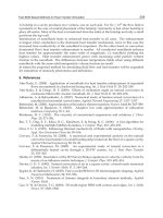
Fig. 1. (a) Aluminum calciner on rollers (side view) showing 10 thermocouples inserted
within the calciner through the Teflon side-wall. (b) Lateral view of the calciner. (c) 10
thermocouples are tied up to the metal rod which is being attached to the teflon wall.
Vertically located, ten holes are also shown in the teflon wall through which thermocouples
are inserted inside the calciner. (d) Another side view showing the internals of the calciner
and the vertical alignment of 10 thermocouples which are visible through the glass window.
We also incorporate cohesive forces between particles in our model using a square-well
potential. In order to compare simulations considering different numbers of particles, the
magnitude of the force was represented in terms of the dimensionless parameter
K = F
cohes
/mg
1
, where K is called the bond number and is a measure of cohesiveness that is

1
Notice that we are not claiming that cohesive forces depend on the particle weight. This is just a convenient way
of defining how strong cohesion is, as compared to the particle weight (i.e. 20 times the weight, 30 times the
weight, etc)
Experimentally Validated Numerical Modeling
of Heat Transfer in Granular Flow in Rotating Vessels

275
independent of particle size, F
cohes

is the cohesive force between particles, and mg is the
weight of the particles. Notice that this constant force may represent short range effects
2

such as electrostatic or van der Waals forces. In this model, the cohesive force (F
cohes
)
between two particles or between a particle and the wall is unambiguously defined in terms
of K. Four friction coefficients need to be defined: particle-particle and particle-wall static
and dynamic coefficients. Interestingly, (and unexpectedly to the authors) all four friction
coefficients turn out to be important to the transport processes.
Heat transport within the granular bed may take place by: thermal conduction within the
solid; thermal conduction through the contact area between two particles in contact; thermal
conduction through the interstitial fluid; heat transfer by fluid convection; radiation heat
transfer between the surfaces of particles. Our work is focused on the first two mechanisms
of conduction which are expected to dominate when the interstitial medium is stagnant and
composed of a material whose thermal conductivity is small compared to that of the
particles. O’Brien (1977) estimated this assumption to be valid as long as (k
S
a / k
f
r ) >> 1,
where a is the contact radius, r is the particle radius of curvature, k
f
denotes the fluid
interstitial medium conductivity and k
S
is the thermal conductivity of the solid granular
material. This condition is identically true when k
f

=0, that is in vacuum.
Heat transport processes are simulated accounting for initial material temperature, wall
temperature, granular heat capacity, granular heat transfer coefficient, and granular flow
properties (cohesion and friction). Heat transfer is simulated using a linear model, where the
flux of heat transported across the mutual boundary between two particles i and j in contact
is described as

()
ij c j i
QHTT
=
−
(3)
Here. T
i
and T
j
are the temperatures of the two particles and the inter-particle conductance
H
c
is:

13
3*
2
4*
N
cS
Fr
Hk

E
⎡
⎤
=
⎢
⎥
⎣
⎦
(4)
where k
S
is the thermal conductivity of the solid material, E* is the effective Young's modulus
for the two particles, and r* is the geometric mean of the particle radii (from Hertz’s elastic
contact theory). The evolution of temperature of particle i from its neighbor (j) is

ii
iii
dT Q
dt C V
ρ
= (5)
Here, Q
i
is the sum of all heat fluxes involving particle i and ρ
i
C
i
V
i
is the thermal capacity of

particle i.
Equations (3-5) can be used to predict the evolution of each particle’s temperature for a
flowing granular system in contact with hot or cold surfaces. The algorithm is used to
examine the evolution of the particle temperature both in the calciner and the double cone
impregnator. This numerical model is developed based on following assumptions:

2
Improvement of this model can be achieved by including electrostatic forces explicitly. We are currently working
on this extension, and the results will be published in a separate article.

Heat Transfer - Mathematical Modelling, Numerical Methods and Information Technology

276
1. Interstitial gas is neglected.
2. Physical properties such a heat capacity, thermal conductivity and Young Modulus are
considered to be constant.
3. During each simulation time step, temperature is uniform in each particle (Biot Number
well below unity).
4. Boundary wall temperature remains constant.
The major computational tasks at each time step are as follows: (i) add/delete contact
between particles, thus updating neighbor lists, (ii) compute contact forces from contact
properties, (iii) compute heat flux using thermal properties (iv) sum all forces and heat
fluxes on particles and update particle position and temperatures, and (v) determine the
trajectory of the particle by integrating Newton’s laws of motion (second order scalar
equations in three dimensions). A central difference scheme, Verlet’s Leap Frog method, is
used here.
The computational conditions and physical parameters considered are summarized in Table
1. Heat transport in alumina is simulated for the experimental validation work, and then
copper is chosen as the material of interest for

0
0.1
0.2
0.3
0.4
0.5
0.6
0.7
0.8
0.9
1
0 200 400 600 800 1000
Time (secs)
(Tavg - To)/(Tw - To)
Alumina
Silica
0
0.01
0.02
0.03
0.04
0.05
0.06
0.07
0.08
024681012
time (secs)
(Tavg - To)/(Tw - To)
Simulation (Alumina)
Experiment (Alumina)

(a) (b)
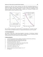
Fig. 2. (a) Variation of average bed temperature with time for alumina and silica; (b)
Evolution of average bed temperature for simulation and experiments with alumina. The fill
level of the calciner is 50% and is rotated at 20rpm in the experiments and simulations
further investigation on baffle size/orientation in calciners and impregnators.We simulated
the flow and heat transfer of 20,000 particles of 1mm size rotated in the calciner equipped
with or without baffle of variable shapes. The calciner consists of a cylindrical 6 inch
diameter vessel with length of 0.6 inches, intentionally flanked with frictionless side walls to
simulate a thin slice of the real calciner, devoid of end-wall effects. Two baffle sizes are
considered (of thicknesses equal to 3cm and 6cm). The initial surface temperature of all the
particles is considered to be 298 K (room temperature) whereas the temperature of the wall
(and the baffle in the impregnator) is considered to be constant, uniform, and equal to 1298
K. The computational conditions and physical parameters considered are summarized in
Table 1. Initially particles were loaded into the system and allowed to reach mechanical
equilibrium. Subsequently, the temperature of the vessel was suddenly raised to a desired
value, and the evolution of the temperature of each particle in the system was recorded as a
function of time.
Experimentally Validated Numerical Modeling
of Heat Transfer in Granular Flow in Rotating Vessels

277
The double cone impregnator model considers flow and heat transfer of 18,000 particles of
3mm diameter in a vessel of 25 cm diameter and 30 cm length. The cylindrical portion of the
impregnator is 25 cm diameter and 7.5 cm long. Each of the conical portions is 11.25 cm long
and makes an angle of 45° with the vertical axis. The diameter at the top or bottom of the
impregnator is 2.5cm The effect of baffle size is investigated in impregnators. Intuitively, the
baffle is kept at an angle 45° with respect to the axis of rotation. The length of the baffle is
25cm, same as the diameter of the cylindrical portion of the impregnator. The width and
thickness of the baffle are equal to one another (square cross section).

In order to describe quantitatively the dynamics of evolution of the granular temperature
field, the following quantities were computed:
- Particle temperature fields vs. time
- Average bed temperature vs. time
- Variance of particle temperatures vs. time
These variables were examined as a function of relevant parameters, and used to examine
heat transport mechanisms in both of the systems of interest here
4. Results and discussions
4.1 Effect of thermal properties in calciners
The effect of thermal conductivity in heat transfer is examined using alumina and silica
particles separately, each occupying 50% of the calciner volume. The calciner is rotated at
the speed of 20 rpm. The average bed temperature (T
avg
) is estimated as the mean of the
readings of the ten thermocouples and scaled with the average wall temperature (T
w
) and
the average initial condition (T
o
) of the particle bed to quantify the effect of thermal
conductivity. In Figure 2a, as expected, alumina with higher thermal conductivity warms up
faster than silica. DEM simulations are performed with the same value for the physical and
thermal properties of the material used in the experiments (for Alumina: thermal
conductivity: k
s
= 35 W/mK and heat capacity: Cp = 875 J/KgK, for Silica: K = 14 W/mK,
Cp = 740 J/KgK). The initial surface temperature of all the particles is considered to be 298 K
(room temperature) whereas the temperature of the wall is kept constant and equal to 398 K
(in isothermal conditions). The DEM simulations predict the temperature of each of the
particles in the system, thus the average bed temperature (T

avg
) in simulation is the mean
value of the predicted temperature of all the particles. Figure (2b) shows the variation of
scaled average bed temperature for both simulation and experiments. The predictions of our
simulation show a similar upward trend to the experimental findings.
4.2 Effect of vessel speed in the calciner
Alumina and silica powders are heated at varying vessel speed of 10, 20 and 30 rpm. The
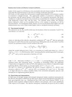
wall is heated and maintained at 100°C. Figure 3(a) and 3(b) show the evolution of average
bed temperature with time as a function of vessel speed for alumina and silica respectively.
The average bed temperatures for all the cases follow nearly identical trends. The external
wall temperature is maintained at a constant temperature of 100°C. Figure (3c) shows the
variation of scaled average bed temperature for simulation.
All experimental temperature measurements were performed every 30 seconds; with a
running time of 1200 seconds. However, each of our simulation runs was performed for
Heat Transfer - Mathematical Modelling, Numerical Methods and Information Technology

278
only 12 seconds. Assuming a dispersion coefficient
2
L
E
T
∼ to be constant [Bird et. al., 1960;
Crank, 1976], where L and T are the length and time scales, respectively, of the microscopic
transitions that generate scalar transport, then the time required to achieve a certain
progress of a temperature profile is proportional to the square of the transport microscale.
The radial transport length scale used in the simulations, if measured in particle diameters,
is much smaller than in the experiment, and correspondingly, the time scale needed to
achieve a comparable progress of the temperature profile is much shorter, as presented in
Figures 3a-c. In fact, the ratio of time scales between the experiment and the simulation

probably is same to the ratio of length scales squared, shown by calculation below.

0
0.1
0.2
0.3
0.4
0.5
0.6
0.7
0.8
0.9
1
0 200 400 600 800 1000
Time (secs)
(Tavg - To)/ (Tw -To)
rpm = 10
rpm = 20
rpm = 30

(a)

0
0.1
0.2
0.3
0.4
0.5
0.6
0.7

0.8
0.9
1
0 200 400 600 800 1000 1200
time (secs)
(Tavg - To)/(Tw-To)
rpm = 10
rpm = 20
rpm = 30
0
0.01
0.02
0.03
0.04
0.05
0.06
0.07
0.08
0.09
024681012
time (secs)
(Tavg -To)/(Tw-To)
rpm = 10
rpm = 20
rpm = 30

(b) (c)
Fig. 3. Variation of temperature with time as a function of vessel speed for (a) Alumina (b)
silica and (c) model with alumina.
In the experiments, the diameter of the vessel (De), duration of the experiment (Te) and

particle size (de) are 6 inches, 1200 seconds and 200 microns (alumina) respectively.
Whereas, in the simulations, the diameter of the vessel (Ds), time of the simulation (Ts) and
particle size (ds) are 6 inches, 12 seconds and 2mm respectively. Ratios of time and length
scales are estimated as below:
Experimentally Validated Numerical Modeling
of Heat Transfer in Granular Flow in Rotating Vessels

279
Ratio of time scales (R
T
):
1200
100
12
Te
Ts
==

Ratio of length scales (R
L
):
6
0.2
10
6
2
e
ee
s
s

s
D
Ld
D
L
d
=
==

Therefore, R
T
= (R
L
)
2
Although there is a big difference in the time scale in the plots of our experiments (Fig. 3a or
Fig. 3b) and simulations (Fig. 3c), they still exhibit the same transport phenomena in
different time scales. The predictions of our simulation show the same upward trend similar
to the experimental findings, even though, they are plotted in different time scales. The
nominal effect of vessel speed on heat transfer was also observed by Lybaert, 1986, in his
experiments with silica sand or glass beads heated in rotary drum heat exchangers.

135
o

(a) (b)
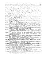
Fig. 4. Baffles are formed with particles glued together (a) square cross-section and
(b) L-shaped cross section.
4.3 Effect of baffles on heat transfer in calciners using a DEM model

T = 0.025000 secs

T = 3.000000 secs

T = 9.000000 secs
T = 0.025000 secs

T = 3.000000 secs

T = 9.000000 secs

T = 0.025000 secs
T = 3.000000 secs
T = 9.000000 secs
time

Fig. 5. Time sequence of axial snapshots
Heat Transfer - Mathematical Modelling, Numerical Methods and Information Technology

280
Section 4.3 is focused on our particle simulations only. After validation of the model,
presented in last two subsections, a parametric study is conducted by varying the size and
the orientation of the baffles of the calciner using the same DEM model. The evolution of
particle temperature is visually track using color-coding. Particles with temperature lower
than 350°K are colored blue; those with temperatures between 350°K and 550°K are painted
cyan; those with temperatures between 550°K and 750°K are colored green and for
temperatures between 750°K and 950°K, particles are colored yellow. Particles with
temperatures higher than 950°K are colored red.
Figure 5 shows a time sequence of axial snapshots of color-coded particles in the calciner.
Time increases from left to right (t = 0, 3 and 9 secs), while the baffle design vary from top to

bottom.
4.3.1 Effect of baffle shape in heat transfer
In this section we study the effect of baffle shape in the calcination process. We do this by
extending the DEM model of a calciner without baffles (which was previously validated) to
one that which now effectively incorporates baffles. In our model, baffles or flights are
attached to the inner wall of the calciner of radius 15cm and length of 1.6cm. Baffles run
longitudinally along the axial direction of the calciner. We consider 8000 copper particles of
radius 2mm heated in the calciner which rotates are 20 rpm for various baffle designs. The
initial temperature of the particles is chosen to be at room temperature (298°K). We simulate
baffles of two different cross sections, i.e. rectangular and L-shaped by rigidly grouping
particles of 2mm size, which perform solid body rotation with the calciner wall. Fig 4
depicts the composition of the different baffles.
We construct the baffle particles purposely overlapping with each other by 10% of their
diameter, to nullify any inter-particle gap which may cause smaller particles to percolate
through the baffle. The square shaped baffle of cross sectional area of approximately 58mm
2

and 340 mm
2
are designed by arranging a matrix of 2 by 2 particles and 5 by 5 particles
respectively. The L-shaped baffle is constructed by 9 particles bonded in a straight line until
the 5
th
particle and then arranging the remaining 4 particles in an angle of 135°. Baffle
particles also remain at the same temperature of the wall, i.e. 1298°K.
For visual representation, particles are color-coded based on their temperature. In Figure 5,
the axial snapshots captured at time t= 0, 1 and 3 revolutions for 3 different baffle
configurations: (i) no baffle (ii) baffles of each 400 mm
2
cross sectional area (iii) 8 L-shaped

flights. The blue core displays the larger mass of particles at initial temperature. This cold
core shrinks with time for all cases, however, the volume of the blue core shrinks faster for
calciner with L shaped baffles. The number of red particles present in the bed increases for
calciners with L-shaped baffles. Thus, increased surface area of the bigger baffle enhances in
heat transfer within the calciners.
The effect of baffle configuration on heat transfer is quantified with our DEM model by
measuring the average bed temperature as a function of time for all baffle configurations.
Average bed temperature rises faster for calciners with L-shaped baffles, as seen in Figure
6(a). The uniformity of the temperature of the particle bed is quantified by estimating the
standard deviation of the temperature of the bed. Figure 6(b) shows the effect of the baffle
configuration on the uniformity of the bed temperature. The L-shaped baffles scoops up
more particles in comparison to the square shaped baffle and helps in breaking the quasi-
static zone in the center of the granular bed and redistributing the particles onto the
cascading layer causing rapid mixing (uniformity) within the bed.
Experimentally Validated Numerical Modeling
of Heat Transfer in Granular Flow in Rotating Vessels

281
300
400
500
600
700
800
900
1000
1100
0 2 4 6 8 10121416
time (sec)
Average Temp (K)

No Baffle
5 by 5 baffle
8 L Flights

0
50
100
150
200
250
300
0246810121416
Time (sec)
Standard deviation of Temp (K)
No Baffle
5 by 5 baffle
8 L Flights

(a) (b)
Fig. 6. (a): Average temperature as function of time for different baffle configurations. (b):
Standard deviation versus time for different baffle configurations.
4.3.2 Effect of baffle size on heat transfer in calciners
The effect of the size of the rectangular baffles/flights is investigated using DEM
simulations. In Figure 7, the axial snapshots captured at time T= 0, 1 and 3 revolutions for 3
different baffle configurations: (i) no baffle (ii) 8 baffles of each 64 mm
2
cross sectional area
(iii) 8 baffles of each 400 mm
2
cross sectional area. In our DEM model, four (2 by 2) and

twenty-five (5 by 5) particles of radius 2 mm are glued together to form each of the baffles in
case (ii) and (iii) respectively. The blue core signifies the mass of particles at initial
temperature.

T = 0.025000 secs
T = 3.000000 secs
T = 9.000000 secs
T = 0.025000 secs
T = 3.000000 secs T = 3.000000 secs
T = 0.025000 secs
T = 3.000000 secs
T = 9.000000 secs
time

Fig. 7. shows a time sequence of axial snapshots of color-coded particles in the calciner.
Time increases from left to right (t = 0, 3 and 9 secs), while the baffle size increases top to
bottom
Heat Transfer - Mathematical Modelling, Numerical Methods and Information Technology

282
This cold core shrinks with time for all cases, but it shrinks faster for a calciner with bigger
baffles. The number of red particles in the bed also increases for calciners with baffles of
bigger sizes. Thus, increased surface area of the bigger baffle enhances heat transfer within
the calciners. The effect of baffle size on heat transfer is quantified by calculating the average
bed temperature as a function of time for all baffle configurations. Average bed temperature
rises faster for calciners with bigger baffles, as seen in Figure 8(a). The uniformity of the
temperature of the particle bed is quantified by estimating the standard deviation of the bed
temperature. Figure 8(b) shows the effect of the baffle size on the uniformity of the bed
temperature, systems with bigger baffles reach uniformity quicker.

300
400
500
600
700
800
900
1000
0246810121416
Time (sec)
Average Bed Temp (K)
No Baffle
2 by 2 Baffle
5 by 5 Baffle

0
50
100
150
200
250
300
0 5 10 15 20
Time (sec)
Standard Deviation of Temp (K)
No Baffle
2 by 2 Baffle
5 by 5 Baffle

(a) (b)

Fig. 8. (a): Average bed temperature as a function of time for different sizes of rectangular
baffles (b): The evolution of standard deviation versus time for different baffle configurations.
4.3.3 Effect of number of baffles/flights on heat transfer in calciners

T = 0.025000 secs

T = 4.500000 secs

T = 9.000000 secs

T = 0.025000 secs

T = 4.500000 secs

T = 9.000000 secs

T = 0.025000 secs

T = 4.500000 secs

T = 9.000000 secs

time

Fig. 9. Evolution of the temperature for non-baffled and baffled calciners (with 4 and 8
flights) at time = 0, 1.5 and 3 revs.
Experimentally Validated Numerical Modeling
of Heat Transfer in Granular Flow in Rotating Vessels

283

The number of baffles is an important geometric parameter for the rotary calciner. The effect
of the parameter has been investigated with a calciner with L-shaped baffles. We calculated
the evolution of the temperature depicted in successive snapshots for 0, 4 and 12 baffles in
Fig 9. There is a cold core which shrinks with time for all the cases, and it shrinks faster for
the calciner with larger number of baffles. The number of red particles present in the bed
also increases for calciners with more baffles. Thus, increase in the number of baffles causes
enhancement in heat transfer within the calciners. The effect of number of baffles on heat
transfer is quantified by calculating the average bed temperature as a function of time for all
baffle configurations. The average temperature of the bed rises faster for calciners with
higher number of baffles. This can be seen in Figure 10(a). The uniformity of the
temperature of the powder bed is quantified by estimating the standard deviation of the
surface temperature of the bed and it is shown in Figure 10(b). It can be seen that the
thermal uniformity of the bed is directly proportional to the number of baffles.

300
400
500
600
700
800
900
1000
1100
02468101214
Time (secs)
Average Bed Temp (K)
No Baffle
4 L Flights
8 L Flights
12 L Flights

0
50
100
150
200
250
300
02468101214
Time (sec)
Standard Deviation of Temp (K)
No Baffle
4 L Flights
8 L Flights
12 L Flights

(a) (b)
Fig. 10. (a): Effect of number of L-Shaped baffles on heat transfer. (b): The evolution of
standard deviation versus time for different baffle configurations
4.3.4 Effect of speed in baffled calciners:
Heat transfer as a function of vessel speed is examined for L-shaped baffles. The evolution
of temperatures of the particles is estimated for calciners with 8 flights/baffles rotated at
different speeds: 10, 20 and 30 rpm (shown in Fig 11). The cold core gets smaller with time
for all the cases, but this reduction is faster for calciners rotated at higher speed. The number
of red particles present in the bed also increases for calciners rotating with higher speed.
Thus, an increase in the speed enhances heat transfer within the calciners. The effect of
speed on heat transfer is quantified by means of the average bed temperature as a function
of time for all baffle configurations. Average bed temperature rises faster for calciners with
higher speeds, as seen in Figure 12(a). This observation contradicts previous observations
for un-baffled calciners. The higher vessel speed ensures more scooping of the material

inside the bed and redistribution of the particles per unit of time, by the L-shaped baffles.
The uniformity of the temperature of the particle bed is quantified by estimating the
standard deviation of the surface temperature of the bed. As expected, bed rotated at higher
speed reaches thermal uniformity faster (see Fig. 12(b)).
Heat Transfer - Mathematical Modelling, Numerical Methods and Information Technology

284


T = 0.025000 secs
T = 4.500000 secs
T = 9.000000 secs
rpm =10

T = 0.025000 secs
T = 4.500000 secs
T = 9.000000 secs
rpm =20

T = 0.025000 secs
T = 4.500000 secs
T = 9.000000 secs
rpm =30

time


Fig. 11. Evolution of temperature for baffled calciners (8 flights) at different rotational
speeds of 10, 20 and 30 rpm, for different values of time = 0, 4.5 and 9 secs.

300
400
500
600
700
800
900
1000
0246810
Time (secs)
Average Bed Temp (K)
10 rpm
20 rpm
30 rpm

0
50
100
150
200
250
300
0246810
Time (secs)
Standard Deviation of Temp (K)
10rpm
20rpm
30rpm

(a) (b)

Fig. 12. (a): Effect of speed on heat transfer for calciners with L-Shaped baffles. (b): The
evolution of the standard deviation versus time for different vessel speeds.
4.3.5. Effect of adiabatic baffles on heat transfer in calciners
In the previous simulations all baffles were always at the wall temperature and enhanced
the heat transfer and thermal uniformity (mixing) in the calciners. However, this can be due
to two distinct effects. The flights not only scoop and redistribute particles enhancing
convective transport, but also heat up the particles during the contact, increasing area for
conductive transport. To nullify the conduction effect and check how flights affect
convective heat transfer, L-shaped baffles were maintained at an adiabatic condition in a
Experimentally Validated Numerical Modeling
of Heat Transfer in Granular Flow in Rotating Vessels

285
particle-baffle contact, dQ = 0 is considered. The 8 flights are thus maintained at the room
temperature (298K) whereas, the wall remains at 1298 K. In Figure 13, the axial snapshots
are displayed at time T= 0, 4 secs and 8 seconds for 2 different baffle configurations: (i) 8 L-
shaped baffles at room temperature (298K) (ii) 8 L-shaped flights at the wall temperature
(1298 K). The blue core signifies the mass of particles at the initial temperature. This cold
core shrinks with time for all the cases, but it shrinks faster for calciners with L-shaped
baffles at wall temperature. The number of red particles present in the bed also increases for
calciners with L-shaped baffles at wall temperature (shown in the left column in Fig 13).


T = 0.000000 secs

T = 0.025000 secs

T = 4.000000 secs

T = 4.025000 secs

T = 8.000000 secs

T = 8.025000 secs

Fig. 13. The axial snapshots of the calciners with cold (left) and hot baffles (right) at different
time intervals.

0
200
400
600
800
1000
1200
0481216
Time (secs)
Average Bed Temp (K)
Cold Flights
Warm Flights
No Flights
0
50
100
150
200
250
300
0246810121416
Time (secs)

Standard Deviation of Temp (K)
Cold Flight
Warm Flight
No flights

(a) (b)
Fig. 14. (a): The evolution of average bed temperature for 8 L shaped cold and warm flights
and unbaffled calciners. (b): The evolution of thermal uniformity for calciners with cold ,
warm baffled and unbaffled flights.
Heat Transfer - Mathematical Modelling, Numerical Methods and Information Technology

286
Thus, heated baffles enhance heat transfer within the calciners. The effect of the temperature
of the baffle on heat transfer is quantified by calculating the average bed temperature as a
function of time for all baffle configurations and comparing it with the temperature profile
of the non-baffled calciner. The average bed temperature rises faster for calciners with L-
shaped baffles at wall temperature, but the calciner with colder baffle shows faster heat
transport than non-baffled calciners (see Figure 14(a)). In Figure 14b, the uniformity of the
temperature of the particle bed is presented by estimating the standard deviation of the
surface temperature of the bed. The calciners with flights are reaching thermal uniformity
faster than the non-baffled calciners. The temperature of the baffle does not cause much
difference in thermal uniformity as both the curves for baffled calciners are very close to
each other (convective mixing effect is independent of baffle temperature)
4.4 Heat transfer of copper particles in the calciner
Initially, 16,000 particles are loaded into the system in a non-overlapping fashion and
allowed to reach mechanical equilibrium under gravitational settling. Subsequently, the
vessel is rotated at given rate, and the evolution of the position and temperature of each
particle in the system is recorded as a function of time. The curved wall is considered to be
frictional. To minimize the finite size effects the flat end walls are considered frictionless and
not participating in heat transfer. A parametric study was conducted by varying thermal

conductivity, particle heat capacity, granular cohesion, vessel fill ratio, and vessel speed of
the calciner. A cohesive granular material (K
cohes
= 75, μ
SP
= 0.8, μ
DP
= 0.6, μ
SW
= 0.8, μ
DW
=
0.8) is considered to examine the effect of thermal properties and the speed of the vessel.
Particles with temperature lower than 350°K are colored blue; those with temperature in
between 350°K and 550°K are considered cyan. Those with temperature between 550°K and
750°K are considered green and for temperatures between 750°K and 950°K are considered
yellow. Those particles with temperature higher than 950°K are colored red.
4.4.1 Effect of thermal conductivity
Three values of thermal conductivity of the solid material are considered: 96.25, 192.5, 385
W/m°K. The calciner is rotated at the speed of 20 rpm. As the heat source is the wall, the
particle bed warms up from the region in contact to the wall. Particle-wall contacts cause the
transport of heat from the wall to the particle bed. With subsequent particle-particle
contacts, heat is transported inside the bed. In Figure 15a, the axial snapshots captured at
time T= 0, 0.5 and 1 revolutions for varying thermal conductivities are displayed. The
combination of heat transfer and convective particle motion results in rings or striations as
the temperature decrease from the wall to the core of the bed. The presence of these
concentric striations signifies that under the conditions examined here, the dominant
mechanism is radial conductive transport of heat from the wall to the core of the bed. The
blue core signifies the mass of particles at initial temperature. This cold core shrinks with
time, as expected; the volume of the blue core shrinks faster for higher particle

conductivities. The average bed temperature is illustrated in Figure (15d). As conductivity
increases, the system exhibits faster heating. The variation of the standard deviation of the
temperature of the bed is illustrated on Fig. 15 (e). Uniformity in the bed temperature
increases with conductivity until the end of 5 revolutions. Finally the bed with higher
conductivity rapidly reaches a thermal equilibrium with the isothermal wall, where all the
particles in bed reach the wall temperature and there is no more heat transfer.
Experimentally Validated Numerical Modeling
of Heat Transfer in Granular Flow in Rotating Vessels

287


T = 0.025000 secs

T = 1.500000 secs

T = 3.000000 secs


T = 1.500000 secs

T = 1.500000 secs

T = 3.025000 secs


T = 0.025000 secs

T = 1.500000 secs

T = 3.000000 secs

k
s


time


(a)

300
400
500
600
700
800
900
1000
012345
Revolutions
Average Bed Temperature (K)
K = 385 W/mK
K = 272 W/mK
K = 192.5 W/mK

0
50
100
150

200
250
300
012345
Revolutions
Standard Deviation of Temp (K)
K = 385 W/mK
K = 272 W/mK
K = 192.5 W/mK


(b) (c)
Fig. 15. (a) shows a time sequence of axial snapshots of color-coded particles in the calciner.
Time increases from left to right (t = 0, 1.5 and 3 secs), while the thermal conductivity
increases from bottom to top (k
s
= 192.5, 272, 385 W/mK). (b) shows the growth of average
bed temperature over time for materials with different conductivity. The granular bed heats
up faster for material with higher conductivity. (c). illustrates the variation of the standard
deviation of particle temperature over time for different conductivities. More uniformity of
temperature in the bed for material of higher thermal conductivity.
A physical formula to fit the simulation prediction is derived based on the Levenberg-
Marquardt method, which uses non-linear least square based regression techniques. This
curve fitting method is employed for the average bed temperature data displayed in Fig 1
for the highest thermal conductivity (k
s
= 385 W/mK). The 3rd order polynomial derived is
as follows
Heat Transfer - Mathematical Modelling, Numerical Methods and Information Technology

288

23
301.92 288.624 45.05 2.9
avg
Tnnn=+ − +
(6)
where T
avg
and n are the average bed temperature and number of revolutions respectively.
The vessel speed for this data is 20 rpm and so n=1 corresponds to 3 seconds. The
correlation coefficient for this fit R = 0.9989. The simulation data and the 3
rd
order least
square fit curve of the data are illustrated in Fig. 15d.To gather an insight of the evolution of
average bed temperatures beyond 5 revolutions, the average bed temperatures at all time
intervals for each of the cases in Fig. 15b is scaled by the corresponding average temperature
at 5 revolutions. In Fig. 15e, almost all of the data points for different conductivity overlap
showing the evolution of average temperature follow the same shape and will reach thermal
equilibrium with the wall at the same rate shown in Fig. 15b.

300
400
500
600
700
800
900
1000
012345

Revolutions
Average Temp (K)
Simulation
NLLS - 3rd Order

0
0.2
0.4
0.6
0.8
1
012345
Revolutions
Tavg/T_5revs
K = 385 W/mK
K = 272 W/mK
K = 192.5 W/mK

(d) (e)
Fig. 15. (d): Comparison of the simulation data (for k
s
= 385 W/mK) and the non-linear least
square fit, (e): Average bed temperature over time for materials with different conductivities.

300
400
500
600
700
800

900
1000
012345
Revolutions
Average Bed Temperature (K)
Cp = 172 J/KgK
Cp = 344 J/KgK
Cp = 688 J/KgK

0
50
100
150
200
250
300
012345
Revolutions
Standard Deviation of Temp (K)
Cp = 172 J/KgK
Cp = 344 J/KgK
Cp = 688 J/KgK

(a) (b)
Fig. 16. (a) Evolution of average bed temperature over time in a calciner, for material with
different heat capacities (Cp= 172, 344, 688 J/KgK). Granular bed heats up faster for material
with lower heat capacity (b) Variation of the standard deviation of particle temperature over
time for different heat capacities. More uniformity of temperature is seen in the bed for
materials of lower heat capacity.
Experimentally Validated Numerical Modeling

of Heat Transfer in Granular Flow in Rotating Vessels

289
4.4.2 Effect of heat capacity
After quantifying the effect of thermal conductivity, the other main thermal property of a
material, heat capacity, is checked. Three values of heat capacity of the granular material are
considered: 172, 344 and 688 J/KgºK, while keeping the thermal conductivity constant at 385
W/m
o
K. Once again, the calciner is rotated at the speed of 20 rpm. Average bed
temperatures are estimated as a function of time (Fig. (16a)). As expected, particles with
lower heat capacity exhibit faster heating. The evolution of the standard deviation of
temperature of the granular bed is illustrated in Figure 16(b). The variability in the bed
temperature is larger for the material with lower heat capacity until 2 revolutions, but at the
end of 5 revolutions, more uniform temperature is observed for the material of lower heat
capacity.
4.4.3 Effect of granular cohesion and friction
The effect of granular cohesion on heat transfer is examined while keeping the thermal
properties constant ( k
s
= 385 W/m
˚
K and Cp = 172 J/Kg
˚
K). As discussed in Section 2, to
simulate different levels of cohesion and friction, the bond number K, the coefficients of
static and dynamic friction between particles (μ
SP
and μ
DP

) and the coefficients of static and
dynamic friction between particle and wall (μ
SW
and μ
DW
) are varied. Heat transfer in
cohesionless particles (K
cohes
= 0, μ
SP
= 0.8, μ
DP
= 0.1, μ
SW
= 0.5, μ
DW
= 0.5) is compared with a
slightly cohesive (K
cohes
= 45, μ
SP
= 0.8, μ
DP
= 0.1, μ
SW
= 0.5, μ
DW
= 0.5) and a very cohesive
material (K
cohes

= 75, μ
SP
= 0.8, μ
DP
= 0.6, μ
SW
= 0.8, μ
DW
= 0.8). The evolution of the average
bed temperature over time is shown in Fig. 17a. For all cases examined here, cohesion does
not cause a significant difference in the temperature profiles. The variability in bed
temperature is quantified by the standard deviation of the particle temperature. In Figure
17b, the variation in standard deviation of temperature for the three values of cohesion is
shown. Once again for the cases examined here, granular cohesion does not have a
significant effect in the uniformity of the particle temperature of the bed.

300
350
400
450
500
550
600
650
700
750
0123456
time (secs)
Average Bed Temp (K)
K = 0

K = 45
K = 75

0
50
100
150
200
250
300
0123456
time (secs)
Standard Deviation of Temp (K)
K = 0
K = 45
K = 75

(a) (b)
Fig. 17. (a) shows the evolution of average bed temperature over time in the calciner, for
materials with different granular cohesion (K
cohes
= 0, 45, 75). (b) illustrates the variation of
the standard deviation of particle temperature over time for different levels of granular
cohesion. Granular cohesion has no significant effect in heat transfer.
Heat Transfer - Mathematical Modelling, Numerical Methods and Information Technology

290
4.4.4. Effect of vessel speed
In order to examine the effect of vessel speed, the most cohesive granular system (K
cohes

=
75) is rotated at three different speeds: 12.5, 20 and 30 rpm, for thermal transport properties
constant and equal to: k
s
= 385 W/m
o
K and C
p
= 172 J/Kg
o
K. Figure 18a displays snapshots
captured at 0, 0.5 and 1 revolutions for varying vessel speeds. The higher vessel speed
applies a higher shear rate to the granular system, causing significant differences in flow
behavior, evident in the different dynamic angle of repose of the bed at each rotational speed.



T = 0.025000 secs

T = 1.500000 secs

T = 3.000000 secs

rpm=20

T = 0.025000 secs

T = 1.000000 secs

T = 2.000000 secs

rpm=30

T = 0.025000 secs

T = 0.750000 secs

T = 1.500000 secs

rpm=40

time


(a)

300
400
500
600
700
800
900
1000
012345
Revolutions
Average Bed Temperature (K)
RPM = 20
RPM = 30
RPM = 40

300
400
500
600
700
800
900
1000
03691215
Time (secs)
Average Bed Temperature (K)
RPM = 20
RPM = 30
RPM = 40

(b) (c)
Fig. 18. (a) shows the time sequence of axial snapshots of color-coded particles in the
calciner. Time increase from left to right hand side (T = 0, 0.5 and 1 revolution), while the
vessel speed increases from top to bottom (20, 30 and 40 rpm). (b) shows the evolution of
average bed temperature versus vessel rotations for different vessel speeds. (c) shows the
average bed temperature profile over real time for different vessel speeds. Rotation speed
increases heat transfer in a per-revolution basis but the effect disappears on a per-time basis.
Experimentally Validated Numerical Modeling
of Heat Transfer in Granular Flow in Rotating Vessels

291
On a per-revolution basis, slower speed caused higher temperature rise (as shown in Fig.
18(b)). A thicker red band of particles (adjacent to the wall) and a smaller blue core are
evident. At slower speeds, each particle has a more prolonged contact with the heated wall,

which contributes to the rapid rise in the temperature. However, when analyzed on per
absolute time basis, the effect of speed dissappers as the average bed temperatures for all
the cases follows nearly identical trends (Fig 18(c)). The standard deviation of the
temperature of the bed is also estimated in per-revolution and per-time basis. While the
temperature of the bed is more uniform at slower speeds on a per revolution basis (Fig.
19(a)). This effect almost disappears on the real time basis (Fig 19(b)).

0
50
100
150
200
250
300
012345
Revolutions
Standard Deviation of Temp (K)
RPM = 20
RPM = 30
RPM = 40

0
50
100
150
200
250
300
350
03691215

Time (Secs)
Standard Deviation of Temp (K)
RPM = 20
RPM = 30
RPM = 40

(a) (b)
Fig. 19. (a) shows the evolution of standard deviation of bed temperature versus vessel
rotations for different vessel speeds. (b) shows the standard deviation of bed temperature
over real time for different vessel speeds. Rotation speed increases the uniformity of bed
temperature in a per revolution basis but the effect almost disappears on a per-time basis.
4.4.5. Effect of fill ratio

300
450
600
750
900
1050
1200
012345
Revolutions
Average Bed Temperature (K)
20% Fill
43% Fill
56% Fill

0
50
100

150
200
250
300
012345
Revolutions
Standard Deviation of Temperature (K)
20% Fill
43% Fill
56% Fill

(a) (b)
Fig. 20. (a) shows the evolution of average bed temperature over time for granular bed of
different volumes (fill % = 20, 43, 56). The granular bed heats up faster for lower fill fraction.
(b) illustrates the variation of the standard deviation of particle temperature over time for
different fill fractions. More uniformity of temperature in the bed of lower fill fraction.
Heat Transfer - Mathematical Modelling, Numerical Methods and Information Technology

292
Three different fill levels, 18%, 43% and 56%, are simulated using 7000, 16000 and 20,000
particles. Once again, the vessel is rotated at 20 rpm. Particle’s thermal transport properties
remain constant at k
s
= 385 W/m
o
K and C
p
= 172 J/Kg°K. Non-cohesive conditions are
considered. In Fig. 20(a), the change in average bed temperature with time is shown as a
function of the fill ratio. As expected, the granular bed with lower fill fraction heats up

faster. Faster mixing is achieved for the lower fill fraction case, which causes rapid heat
transfer from the vessel wall to the granular bed. The temperature is more uniform for lower
fill fraction at the end of 5 revolutions (Fig 20(b)).
4.5 Heat transfer in a double cone impregnator

300
400
500
600
700
800
900
012345
Revolutions
Average Bed Temp (K)
Ks = 385 W/mK
Ks = 272 W/mK
Ks = 192.5 W/mK

0
50
100
150
200
250
012345
Revolutions
Standard Deviation of Temp(K)
Ks = 385 W/mK
Ks = 272.5 W/mK

Ks = 192.5 W/mK

(a) (b)

300
400
500
600
700
800
900
1000
012345
Revolutions
Average Bed Temp (K)
Ks = 385 W/mK
Ks = 272 W/mK
Ks = 192.5 W/mK

0
50
100
150
200
250
012345
Revolutions
Standard Deviation of Temp (K)
Ks = 385 W/mK
Ks = 272.5 W/mK

Ks = 192.5 W/mK

(c) (d)
Fig. 21. (a) shows the growth of the average bed temperature over time in a non-baffled
impregnator, for materials with different thermal conductivities (k
s
= 192.5, 272, 385 W/mK).
(b) shows the growth of the average temperature of the bed over time in baffled
impregnator, for materials with different thermal conductivities (k
s
= 192.5, 272, 385 W/mK).
(c) illustrates the variation of the standard deviation of particle temperature in the non-
baffled impregnator over time for different thermal conductivities. (d) illustrates the
variation of the standard deviation of particle temperature over time for different thermal
conductivities for a baffled vessel. Granular bed heats up faster for material with higher
thermal conductivity.
Experimentally Validated Numerical Modeling
of Heat Transfer in Granular Flow in Rotating Vessels

293
We simulate the flow and heat transfer of 18,000 particles of 3mm size rotated in a double
cone impregnator equipped with a baffle of variable size. Initially, particles are loaded into
the system (with and without baffles) and allowed to reach mechanical equilibrium.
Subsequently, the temperature of the vessel (and the baffle) is raised to the desired value of
1298°K, and the evolution of the temperature of each particle in the system is recorded as a
function of time. All impregnator walls are considered to be frictional in the simulation.
Coefficients of static friction between particles and particle-wall are considered to be 0.8 and
0.5 respectively. Coefficient of dynamic friction is considered to be the same as those of
static friction for simplicity.
Firstly, the effects of thermal conductivity and heat capacity on temperature are examined.

Subsequently, the impact of the vessel speed and baffle size on heat transfer rate and
temperature field uniformity are examined. Three cases are considered: (a) no baffle, (b)
baffle with 9 cm
2
cross-section (c) baffle with 36 cm
2
cross-section. Particles in all the
impregnator simulations are considered non-cohesive. Once again, the initial temperature of
all the particles are considered to be at 298°K (room temperature) whereas the temperature
of the wall (and the baffle if present) is considered to be at 1298°K (and in isothermal
condition). Particles with temperature lower than 400°K are colored blue, while those with
temperature in between 400°K and 600°K are colored green; those with temperature in
between 600°K and 900°K are colored yellow, and those with temperatures higher than
900°K are colored red.
4.5.1 Effect of thermal conductivity
Higher thermal conductivity favored the transfer of heat and enhanced temperature
uniformity in calciner flows. Impregnators and calciners both tumble but have different
shapes. The effect of thermal conductivity on granular bed temperature is quantified for
non-baffled and baffled impregnators. Three values of thermal conductivity (k
s
) of the
material are considered: 96.25, 192.5 and 385 W/m°K. All three simulations are performed at
20 rpm. The evolution of the average bed temperature as a function of thermal conductivity
is shown in Fig. 21a (un-baffled impregnator) and 21b (baffled impregnator with baffle
cross-sectional area of 9 cm
2
). More conductive particles exhibit faster heating in both cases.
The standard deviation plots corresponding to particle temperature for the non-baffled and
baffled impregnators are shown in Fig 21c and 21d. In the first three revolutions, we observe
more uniform (lower standard deviation) temperature for the cases with lower conductivity.

At later times, as most particles reach high temperatures, all the curves show low values of
standard deviation (not shown). More uniform temperature is attained in the bed of highest
conductivity (k
s
= 385 W/mK) after 3 revolutions (Figs. 21c and 21d).
4.5.2 Effect of heat capacity
Similar to the transient heat transfer analysis of the calciner, the effect of heat capacity is also
quantified for non-baffled and baffled impregnators. Three values of heat capacity are
considered: 172, 344 and 688 J/Kg°K. The coefficient of thermal conductivity is kept constant
at 385 W/m°K. These simulations are performed at a vessel speed of 20 rpm. The evolution
of the average bed temperature over time is depicted in Fig. 22(a). As expected, the lower
the heat capacity, the faster the rise in bed temperature. The variability of the bed
temperature is higher for material with higher heat capacity (see Fig. 22(b)).