Mass Transfer in Multiphase Systems and its Applications Part 18 ppt

Impact of Mass Transfer on Modelling and Simulation of Reactive Distillation Columns

669
lower branch and a decrease of the mass transfer coefficient caused an increase of the
conversion in steady states located on the lower branch; however the number of steady
states and quality of higher steady states located on isolas did not change. An interesting
result is depicted in Fig. 11b. If the Chen-Chuang method is used to calculate the mass
transfer coefficients, only one steady state is predicted for the operational feed flow rate of
butenes (1900 kmol h
-1
). Multiple steady states are predicted only for a short interval of
butenes feed flow rate (approximately 1500- 1750 kmol h
-1
). However, a 10 % increase of the
mass transfer coefficients above the value calculated using the Chen- Chuang method
(dashed line in Fig. 11b) caused that multiple steady states appeared for the operational feed
flow rate of butenes and the shape of the calculated curves were significantly similar to
those calculated using the AICHE method. On the other hand, a 10% decrease of the mass
transfer coefficients below the value calculated using the Chen- Chuang method (dash-
dotted line in Fig. 11a) caused that multiple steady states almost completely disappeared.

1000 1250 1500 1750 2000 2250 2500
0.2
0.3
0.4
0.5
0.6
0.7
0.8
0.9
1.0

1.5xD
L
1.2xD
L
1.0xD
L
0.8xD
L
0.5xD
L
a)
convesr
i
on o
f

i
so-
b
utene
/

[
-
]
butenes feed flow rate / [kmol/h]

1000 1250 1500 1750 2000 2250 2500
0.2
0.3

0.4
0.5
0.6
0.7
0.8
0.9
1.0
b)
1.5xD
L
1.2xD
L
1.0xD
L
0.8xD
L
0.5xD
L
convesr
i
on o
f

i
so-
b
u
t
ene
/

[
-
]
butenes feed flow rate / [kmol/h]


1000 1250 1500 1750 2000 2250 2500
0.4
0.5
0.6
0.7
0.8
0.9
1.0
c)
1.5xD
L
1.2xD
L
1.0xD
L
0.8xD
L
0.5xD
L
convesrion of iso-butene / [-]
butenes feed flow rate / [kmol/h]

1000 1250 1500 1750 2000 2250 2500

0.7
0.8
0.9
1.0
1.5xD
L
1.2xD
L
1.0xD
L
0.8xD
L
0.5xD
L
d)
convesr
i
on o
f

i
so-
b
utene
/

[
-
]
butenes feed flow rate / [kmol/h]

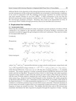
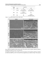
Fig. 12. Conversion of isobutene vs. butenes feed flow rate solution diagrams calculated
using different liquid phase diffusion coefficient (±20%, ±50%) for all investigated models: a)
Model 1, b) Model 2, c) Model 3 , d) Model 4
From this follows that a 10 % change of the value of mass transfer coefficients may even
affect the number of the predicted steady states and consequently the whole prediction of
the reactive distillation column behaviour during dynamic change of parameters.
Investigations presented in Fig. 11 were made under the assumption that all binary mass
Mass Transfer in Multiphase Systems and its Applications

670
transfer coefficients (as well as the liquid in the gas phase) are by 10 % higher or lower than
those calculated using empirical correlations (AICHE, Chen-Chuang). This is a very rough
assumption which implies a potential uncertainty of the input parameters (diffusivity in the
liquid or vapour phase, surface tension, viscosity, density, etc.) needed for the calculation of
the mass transfer coefficients according to the correlations. It is important to note that each
input parameter needed for the mass transfer coefficient calculation may influence the
general NEQ model steady state prediction relatively significantly. Fig. 12 shows isobutene
conversion dependence on the butenes feed flow rate calculated using a) Model 1, b) Model
2, c) Model 3 , d) Model 4, whereby several different values of the diffusion coefficients in
the liquid phase were used in each model. To calculate the diffusion coefficients in a dilute
liquid mixture, the Wilke-Chang (1955) correlation was used, which corresponds to the solid
lines in Fig. 12a-d. To show the effect of of the diffusion coefficient uncertainty on the NEQ
models steady state prediction, a 20 % and 50 % increase as well as decrease of the
calculated diffusion coefficients was assumed. From Fig. 12 follows that the effect of the
liquid phase diffusion coefficients on the steady states prediction using different models for
mass transfer coefficient prediction is significantly different. The most distinguishable
influence can be noticed using Model 3 (i.e., the Chen- Chuang method, see Fig. 12c) where
the decrease of the diffusion coefficients led to notable reduction of the multiple steady state
zone and the course of the curves was similar to that predicted by Method 4 (i.e., the

Zuiderweg method, see Fig. 12d). On the other hand, the increase of the diffusion
coefficients led to isola closure and creation of a multiplicity zone similar to that predicted
by Method 1 (i.e., the AICHE method, see Fig. 12a) and Method 2 (i.e., the Chan-Fair
method, see Fig. 12b). The effect of diffusion coefficients variation is very similar for Method
1 and Method 2 whereas the same equation was used for the number of transfer units in the
liquid phase. Method 4 (i.e., the Zuiderweg method, see Fig. 12d) shows the smallest
dependence on the diffusion coefficients change.
4. Conclusion
A reliable prediction of the reactive distillation column behaviour is influenced by the
complexity of the mathematical model which is used for its description. For reactive
distillation column modelling, equilibrium and nonequilibrium models are available in
literature. The EQ model is simpler, requiring a lower number of the model parameters; on
the other hand, the assumption of equilibrium between the vapour and liquid streams
leaving the reactor can be difficult to meet, especially if some perturbations of the process
parameters occur. The NEQ model takes the interphase mass and heat transfer resistances
into account. Moreover, the quality of a nonequilibrium model differs in dependence of the
description of the vapour–liquid equlibria, reaction equilibria and kinetics (homogenous,
heterogeneous reaction, pseudo-homogenous approach), mass transfer (effective diffusivity
method, Maxwell - Stefan approach) and hydrodynamics (completely mixed vapour and
liquid, plug-flow vapour, eddy diffusion model for the liquid phase, etc.). It is obvious that
different model approaches lead more or less to different predictions of the reactive
distillation column behaviour. As it was shown, different correlations used for the
prediction of the mass transfer coefficient estimation lead to significant differences in the
prediction of the reactive distillation column behaviour. At the present time, considerable
progress has been made regarding the reactive distillation column hardware aspects (tray
Impact of Mass Transfer on Modelling and Simulation of Reactive Distillation Columns

671
design and layout, packing type and size). If mathematical modelling is to be a useful tool
for optimisation, design, scale-up and safety analysis of a reactive distillation column, the

correlations applied in model parameter predictions have to be carefully chosen and
employed for concrete column hardware. A problem could arise if, for a novel column
hardware, such correlations are still not available in literature, e.g. the correlation and model
quality progress are not equivalent to the hardware progress of the reactive distillation
column.
As it is possible to see from Figs. 8a and b, for given operational conditions and a “good”
initial guess of the calculated column variables (V and L concentrations and temperature
profiles, etc.), the NEQ model given by a system of non-linear algebraic equations
converged practically to the same steady state with high conversion of isobutene (point A in
Fig. 8) with all assumed correlations. If a “wrong” initial guess was chosen, the NEQ model
can provide different results according to the applied correlation: point A for Models 3 and
4 with high conversion of isobutene, point B for Model 2 and point C for Model 1. Therefore,
the analysis of multiple steady-states existence has to be done as the first step of a safety
analysis. If we assume the operational steady state of a column given by point A, and start
to generate HAZOP deviations of operational parameters, by dynamic simulation, we can
obtain different predictions of the column behaviour for each correlation, see Fig. 9a. Also,
dynamic simulation of the column start-up procedure from the same initial conditions (for
NEQ model equations) results in different steady states depending on chosen correlation,
see Fig. 9b.
Our point of view is that of an engineer who has to do a safety analysis of a reactive
distillation column using the mathematical model of such a device. Collecting literature
information, he can discover that there are a lot of papers dealing with mathematical
modelling. As was mentioned above, Taylor and Krishna (Taylor & Krishna, 2000) cite over
one hundred papers dealing with mathematical modelling of RD of different complexicity.
And there is a problem: which model is the best and how to obtain parameters for the
chosen model. There are no general guidelines in literature. Using correlations suggested by
authorities, an engineer can get into troubles. If different models predict different multiple
steady states in a reactive distillation column for the same column configuration and the
same operational conditions, they also predict different dynamic behaviour and provide
different answers to the deviations generated by HAZOP. Consequently, it can lead to

different definitions of the operator’s strategy under normal and abnormal conditions and in
training of operational staff.
5. Acknowledgement
This work was supported by the Slovak Research and Development Agency under the
contract No. APVV-0355-07.
6. Nomenclature
A
b

bubbling area of a tray, m
2
(Table 4)
A
h

hole area of a sieve tray, m
2
(Table 4)
A
interfacial area per unit volume of froth, m
2
m
-3
(Eqs. (15),(16))
a
I

net interfacial area, m
2

Mass Transfer in Multiphase Systems and its Applications

672
b
weir length per unit of bubbling area, m
-1
(Table 4)
C
p

heat capacity, J mol
-1
K
-1

c
molar concentration, mol m
-3

E

energy transfer rate, J s
-1

D
Fick’s diffusivity, m
2
s
-1

D
Maxwell-Stefan diffusivity, m
2
s
-1

F
feed stream, mol s
-1

F
f

fractional approach to flooding (Table 4)
FP
flow parameter (Table 4)
F
s

superficial F factor, kg
0.5
m
-0.5
s
-1
(Table 4)
H
molar enthalpy, J mol
-1

Δ
r
H
reaction enthalpy, J mol
-1

h
heat transfer coefficient, J s
-1
m
-2
K
-1

h
L

clear liquid height, m (Table 4)
h
w

exit weir height, m (Table 4)
J
molar diffusion flux relative to the molar average velocity, mol m
-2
s
-1

K
i

vapour-liquid equilibrium constant for component i
[k]
matrix of multicomponent mass transfer coefficients, m s
-1

L
liquid flow rate, mol s
-1

Le
Lewis number (
11 1
p
CD
λρ
−
−−
)
M
mass flow rates, kg s
-1
(Table 4)
N
number of transfer units
N
F

number of feed streams
N

I

number of components
N
R

number of reactions
N
transfer rate, mol s
-1

n
number of stages
P
pressure of the system, Pa
PF
Pointing correction
PΔ
pressure drop, Pa
p
hole pitch, m (Table 4)
Q
heating rate, J s
-1

Q
L

volumetric liquid flow rate, m
3

s
-1
(Table 4)
Q
V

volumetric vapour flow rate, m
3
s
-1
(Eq.(17))
[R]
matrix of mass transfer resistances, s m
-1

r
ratio of side stream flow to interstage flow
Sc
V

Schmidt number for the vapour phase (Table 4)
T
temperature, K
t
time, s
t
residence time, s (Table 4)
Impact of Mass Transfer on Modelling and Simulation of Reactive Distillation Columns

673

U
molar hold-up, mol
u
s

superficial vapour velocity, m s
-1

u
sf

superficial vapour velocity at flooding, m s
-1

V
vapour flow rate, mol s
-1

W
weir length, m (Table 4)
x
mole fraction in the liquid phase
y
mole fraction in the vapour phase
Z
the liquid flow path length, m (Table 4)
z
P

mole fraction for phase P

Greek letters
β

fractional free area (Table 4)
[
Γ
]
matrix of thermodynamic factors
ε

heat transfer rate factor
κ

binary mass transfer coefficient, m s
-1

λ

thermal conductivity, W m
-1
K
-1

μ

viscosity of vapour and liquid phase, Pa s
ν

stoichiometric coefficient
ξ



reaction rate, mol s
-1

ρ

vapour and liquid phase density, kg m
-3
(Table 4)
σ

surface tension, N m
-1

Superscripts
o
initial conditions
I referring to the interface
L referring to the liquid phase
V referring to the vapour phase
Subscripts
av averaged value
f feed stream index
i component index
j stage index
m mixture property
r
reaction index
t referring to the total mixture

7. References
AICHE (1958). AICHE Bubble Tray Design Manual, AIChE, New York
Baur, R., Higler, A. P., Taylor, R. & Krishna, R. (2000). Comparison of equilibrium stage and
nonequilibrium stage models for reactive distillation,
Chemical Engineering Journal,
76(
1), 33-47; ISSN: 1385-8947.
Mass Transfer in Multiphase Systems and its Applications

674
Fuller, E. N., Schettler, P. D. & Gibbings, J. C. (1966). A new method for prediction of binary
gas-phase diffusion coefficints,
Industrial & Enegineering Chemistry, 58(5), 18-27;
ISSN: 0888-5885.
Górak, A. (2006). Modelling reactive distillation.
Proceedings of 33rd International Conference of
Slovak Society of Chemical Engineering
, ISBN:80-227-2409-2, Tatranské Matliare,
Slovakia, May 2006, Slovak University of Technology, Bratislava, SK, in Publishing
House of STU.
Chan, H. & Fair, J. R. (1984). Prediction of point efficiencies on sieve trays. 2.
Multicomponent systems,
Industrial & Engineering Chemistry Process Design
Development,
23(4), 820-827; ISSN: 0196-4305.
Chen, G. X. & Chuang, K. T. (1993). Prediction of point efficiency for sieve trays in
distillation,
Industrial & Engineering Chemistry Research, 32, 701-708; ISSN: 0888-5885.
Jacobs, R. & Krishna, R. (1993). Multiple Solutions in Reactive Distillation for Methyl tert-
Butyl Ether Synthesis,

Industrial & Engineering Chemistry Research, 32(8), 1706-1709;
ISSN: 0888-5885.
Jones Jr., E. M. (1985). Contact structure for use in catalytic distillation, US Patent 4536373.
Kletz, T. (1999).
HAZOP and HAZAN, Institution of Chemical Engineers, ISBN: 978-
0852954218
Kooijman, H. A. & Taylor, R. (1995). Modelling mass transfer in multicomponent
distillation,
The Chemical Engineering Journal, 57(2), 177-188; ISSN: 1385-8947.
Kooijman, H. A. & Taylor, R. (2000).
The ChemSep book, Libri Books on Demand, ISBN: 3-
8311-1068-9, Norderstedt
Kotora, M., Švandová, Z. & Markoš, J. (2009). A three-phase nonequilibrium model for
catalytic distillation,
Chemical Papers, 63(2), 197-204; ISSN: 0336-6352.
Krishna, R. & Wesselingh, J. A. (1997). The Maxwell-Stefan approach to mass transfer,
Chemical Engineering Science, 52(6), 861-911; ISSN: 0009-2509.
Krishnamurthy, R. & Taylor, R. (1985a). A nonequilibrium stage model of multicomponent
separation processes I-Model description and method of solution,
AIChE Journal,
31(
3), 449-456; ISSN:1547-5905
Krishnamurthy, R. & Taylor, R. (1985b). A nonequilibrium stage model of multicomponent
separation processes II-Comparison with experiment,
AIChE Journal, 31(3), 456-465;
ISSN:1547-5905
Kubíček, M. (1976). Algorithm 502. Dependence of solution of nonlinear systems on a
parameter [C5],
Transaction on Mathematical Software, 2(1), 98-107; ISSN 0098-3500.
Labovský, J., Švandová, Z., Markoš, J. & Jelemenský (2007a). Mathematical model of a

chemical reactor-Useful tool for its safety analysis and design,
Chemical Engineering
Science,
62, 4915- 4919; ISSN: 0009-2509.
Labovský, J., Švandová, Z., Markoš, J. & Jelemenský (2007b). Model-based HAZOP study of
a real MTBE plant,
Journal of Loss Prevention in the Process Industries, 20(3), 230-237;
ISSN: 0950-4230
Marek, M. & Schreiber, I. (1991).
Chaotic Behaviour of Deterministic Dissipative Systems,
Academia Praha, ISBN: 80-200-0186-7, Praha
Mohl, K D., Kienle, A., Gilles, E D., Rapmund, P., Sundmacher, K. & Hoffmann, U. (1999).
Steady-state multiplicities in reactive distillation columns for the production of fuel
Impact of Mass Transfer on Modelling and Simulation of Reactive Distillation Columns

675
ethers MTBE and TAME: theoretical analysis and experimental verification,
Chemical Engineering Science, 54(8), 1029-1043; ISSN: 0009-2509.
Molnár, A., Markoš, J. & Jelemenský, L. (2005). Some considerations for safety analysis of
chemical reactors,
Trans IChemE, Part A: Chemical Engineering Research and Design,
83(
A2), 167-176; ISSN: 0263-8762.
Noeres, C., Kenig, E. Y. & Gorak, A. (2003). Modelling of reactive separation processes:
reactive absorption and reactive distillation,
Chemical Engineering and Processing,
42(
3), 157-178; ISSN: 0255-2701.
Perry, R. H., Green, D. W. & Maloney, J. O. (1997).
Perry’s Chemical Engineers’ Handbook,

McGraw-Hill, ISBN 0-07-049841-5, New York
Rehfinger, A. & Hoffmann, U. (1990). Kinetics of methyl tertiary butyl ether liquid phase
synthesis catalyzed by ion exchange resin I. Intrinsic rate expression in liquid
phase activities,
Chemical Engineering Science, 45(6), 1605-1617; ISSN: 0009-2509.
Reid, R. C., Prausnitz, J. M., Sherwood, T. K. (1977).
The Properties of Gases and Liquids,
McGraw-Hill, ISBN: 0-07-051790-8, New York
Sláva, J., Jelemenský, L. & Markos, J. (2009). Numerical algorithm for modeling of reactive
separation column with fast chemical reaction,
Chemical Engineering Journal, 150(1),
252-260; ISSN: 1385-8947.
Sláva, J., Svandová, Z. & Markos, J. (2008). Modelling of reactive separations including fast
chemical reactions in CSTR,
Chemical Engineering Journal, 139(3), 517-522; ISSN:
1385-8947.
Sundmacher, K. & Kienle, A. (2002).
Reactive Distillation, Status a Future Directions, Wiley-
VCH Verlag GmbH & Co. KGaA, ISBN: 3-527-60052-3, Weinheim
Švandová, Z., Jelemenský, Markoš, J. & Molnár, A. (2005b). Steady state analysis and
dynamical simulation as a complement in the HAZOP study of chemical reactors,
Trans IChemE, Part B: Process Safety and Environmental Protection, 83(B5), 463 - 471;
ISSN: 0957-5820.
Švandová, Z., Labovský, J., Markoš, J. & Jelemenský, Ľ. (2009). Impact of mathematical
model selection on prediction of steady state and dynamic behaviour of a reactive
distillation column,
Computers & Chemical Engineering, 33, 788-793; ISSN: 0098-1354.
Švandová, Z., Markoš, J. & Jelemenský (2005a). HAZOP analysis of CSTR with utilization of
mathematical modeling,
Chemical Papers, 59(6b), 464-468; ISSN: 0336-6352.

Švandová, Z., Markoš, J. & Jelemenský, Ľ. (2008). Impact of mass transfer coefficient
correlations on prediction of reactive distillation column behaviour,
Chemical
Engineering Journal,
140(1-3), 381-390; ISSN: 1385-8947.
Taylor, R., Kooijman, H. A. & Hung, J S. (1994). A second generation nonequilibrium model
for computer simulation of multicomponent separation processes,
Computers &
Chemical Engineering,
18(3), 205-217; ISSN: 0098-1354.
Taylor, R. & Krishna, R. (1993).
Multicomponent Mass Transfer, John Wiley & Sons, Inc., ISBN:
0-471-57417-1, New York
Taylor, R. & Krishna, R. (2000). Modelling reactive distillation,
Chemical Engineering Science,
55(22), 5183-5229; ISSN: 0009-2509.
Wesselingh, J. A., Krishna, R. (1990).
Mass Transfer, Ellis Horwood Ltd, ISBN:978-
0135530252, Chichester, England
Mass Transfer in Multiphase Systems and its Applications

676
Wilke, C. R. & Chang, P. (1955). Correlations of Diffusion Coefficients in Dilute Solutions,
AiChE Journal, 1(2), 264-270; ISSN:1547-5905
Zuiderweg, F. J. (1982). Sieve trays : A view on the state of the art,
Chemical Engineering
Science,
37(10), 1441-1464; ISSN: 0009-2509.
29
Mass Transfer through

Catalytic Membrane Layer
Nagy Endre
University of Pannonia, Research Institute of Chemical and Process Engineering
Hungary
1. Introduction
The catalytic membrane reactor as a promising novel technology is widely recommended
for carrying out heterogeneous reactions. A number of reactions have been investigated by
means of this process, such as dehydrogenation of alkanes to alkenes, partial oxidation
reactions using inorganic or organic peroxides, as well as partial hydrogenations, hydration,
etc. As catalytic membrane reactors for these reactions, intrinsically catalytic membranes can
be used (e.g. zeolite or metallic membranes) or membranes that have been made catalytic by
dispersion or impregnation of catalytically active particles such as metallic complexes,
metallic clusters or activated carbon, zeolite particles, etc. throughout dense polymeric- or
inorganic membrane layers

(Markano & Tsotsis, 2002). In the majority of the above
experiments, the reactants are separated from each other by the catalytic membrane layer. In
this case the reactants are absorbed into the catalytic membrane matrix and then transported
by diffusion (and in special cases by convection) from the membrane interface into catalyst
particles where they react. Mass transport limitation can be experienced with this method,
which can also reduce selectivity. The application of a sweep gas on the permeate side
dilutes the permeating component, thus increasing the chemical reaction gradient and the
driving force for permeation (e.g. see Westermann and Melin, 2009). At the present time, the
use of a flow-through catalytic membrane layer is recommended more frequently for
catalytic reactions (Westermann and Melin, 2009). If the reactant mixture is forced to flow
through the pores of a membrane which has been impregnated with catalyst, the intensive
contact allows for high catalytic activity with negligible diffusive mass transport resistance.
By means of convective flow the desired concentration level of reactants can be maintained
and side reactions can often be avoided (see review by Julbe et al., 2001). When describing
catalytic processes in a membrane reactor, therefore, the effect of convective flow should

also be taken into account. Yamada et al., (1988) reported isomerization of 1-butene as the
first application of a catalytic membrane as a flow-through reactor. This method has been
used for a number of gas-phase and liquid-phase catalytic reactions such as VOC
decomposition (Saracco & Specchia, 1995), photocatalytic oxidation (Maira et al., 2003),
partial oxidation

(Kobayashi et al., 2003), partial hydrogenation (Lange et a., 1998; Vincent &
Gonzales, 2002; Schmidt et al., 2005) and hydrogenation of nitrate in water (Ilinitch et al.,
2000).
From a chemical engineering point of view, it is important to predict the mass transfer rate
of the reactant entering the membrane layer from the upstream phase, and also to predict
Mass Transfer in Multiphase Systems and its Applications

678
the downstream mass transfer rate on the permeate side of the catalytic membrane as a
function of the physico-chemical parameters. The outlet mass transfer rate should generally
be avoided. The mathematical description of the mass transport enables the reader to choose
the operating conditions in order to minimize the outlet mass transfer rate. If this transfer
(permeation) rate is known as a function of the reaction rate constant, it can be substituted
into the boundary conditions of the full-scale differential mass balance equations for the
upstream and/or the downstream phases. Such kind of mass transfer equations can not be
found in the literature, yet. For their description, two types of membrane reactors should
generally be distinguished, namely intrinsically catalytic membrane and membrane layer
with dispersed catalyst particle, either nanometer size or micrometer size catalyst particles.
Basically, in order to describe the mass transfer rate, a heterogeneous model can be used for
larger particles and/or a pseudo-homogeneous one for very fine catalyst particles (Nagy,
2007). Both approaches, namely the heterogeneous model for larger catalyst particles and
the homogeneous one for submicron particles, will be applied for mass transfer through a
catalytic membrane layer. Mathematical equations have been developed to describe the
simultaneous effect of diffusive flow and convective flow and this paper analyzes mass

transport and concentration distribution by applying the model developed.
Membrane bioreactor (MBR) technology is advancing rapidly around the world both in
research and commercial applications (Strathman et al., 2006; Yang and Cicek, 2006; Giorno
and Drioli, 2000; Marcano and Tsotsis, 2002). Integrating the properties of membranes with
biological catalyst such as cells or enzymes forms the basis of an important new technology
called membrane bioreactor. Membrane layer is especially useful for immobilizing whole
cells (bacteria, yeast, mammalian and plant cells) (Brotherton and Chau, 1990; Sheldon and
Small, 2005), bioactive molecules such as enzymes (Rios et al., 2007; Charcosset, 2006;
Frazeres and Cabral, 2001) to produce wide variety of chemicals and substances. The main
advantages of the membrane, especially the hollow fiber, bioreactor are the large specific
surface area (internal and external surface of the membrane) for cell adhesion or enzyme
immobilization; the ability to grow cells to high density; the possibility for simultaneous
reaction and separation; relatively short diffusion path in the membrane layer; the presence
of convective velocity through the membrane if it is necessary in order to avoid the nutrient
limitation (Belfort, 1989; Piret and Cooney, 1991; Sardonini and DiBiasio, 1992). This work
analyzes the mass transport through biocatalytic membrane layer, either live cells or
enzymes, inoculated into the shell and immobilized within the membrane matrix or in a thin
layer at the membrane matrix matrix-shell interface. Cells are either grown within the fibers
with medium flow outside or across the fibers while wastes and desired products are
removed or grown in the extracapillary space with medium flow through the fibers and
supplied with oxygen and nutrients (Fig. 12 illustrates this situation). The performance of a
hollow-fiber or sheet bioreactor is primarily determined by the momentum and mass
transport rate (Calabro et al., 2002; Godongwana et al., 2007) of the key nutrients through
the bio-catalytic membrane layer. Thus, the operating conditions (trans-membrane pressure,
feed velocity), the physical properties of membrane (porosity, wall thickness, lumen radius,
matrix structure, etc.) can considerably influence the performance of a bioreactor, the
effectiveness of the reaction. The introduction of convective transport is crucial in
overcoming diffusive mass transport limitation of nutrients (Nakajima and Cardoso, 1989)
especially of the sparingly soluble oxygen. Several investigators modeled the mass transport
through this biocatalyst layer, through enzyme membrane layer (Ferreira et al., 2001; Long

et al., 2003; Belfort, 1989; Hossain and Do, 1989; Calabro et al., 2002; Waterland et al., 1975;
Mass Transfer through Catalytic Membrane Layer

679
Salzman et al., 1999; Carvalho et al, 2000) or cell culture membrane layer (Melo and Oliveira,
2001; Brotherton and Chau, 1990, 1996; Piret and Cooney, 1991; Sardonini and Dibiasio,
1992; Lu et al., 2001; Schonberg and Belfort, 1987). These studies analyze both the mass
transport through the membrane and the bulk phase concentration change. Against these
detailed studies, there are not known mass transfer equations which define the mass
transfer rate through a biocatalytic membrane layer, in closed forms as a function of the
transport parameters as membrane Peclet number, reaction rate modulus as well as the
Peclet number of the concentration boundary layer. These equations could then be replaced
in the full-scale mass transfer models in order to predict the concentration distribution in the
bulk liquid phase.
When someone knows the mass transfer rate through the membrane, these rate equations
now can be put into the full-scale mass balance equation as boundary value to describe the
concentration distribution on the lumen side, feed side or on the shell side, permeate side.
The full-scale description of flow in crossflow filtration tubular membrane or in flat sheet
membrane is also very often the object of investigations (Damak et al., 2004). A fluid
dynamic description of free flows is usually easy to perform, and in a great majority of
examples, the well known Navier-Stokes equations can be used to coupling Darcy’s law and
the Navier-Stokes equations (Mondor & Moresoli, 1999; Damak et al., 2004). A steady-state,
laminar, incompressible, viscous and isothermal flow in a cylindrical tube with a permeable
wall is considered. The Navier-Stokes equation and Darcy’s law describe the transfer in the
tube and in the porous wall, respectively.
2. Mass transfer through membrane reactor
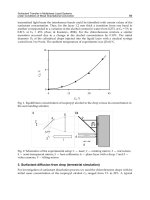
Six membrane reactor concepts can be considered related to the catalysts location in the
membrane modules (Seidel-Morgenstern, 2010). Topics of this paper are the concept when
the catalyst particles are dispersed in the membrane matrix (the membrane serves an active
contactor) or the membrane layer is intrinsically catalytic. This concept is illustrated in Fig.

1. The reactants are fed into the reactor from different sides and react within the membrane.

catalyst
c
C
A
B
J
B
J
A + B
C

Fig. 1. Schematic illustration of catalytic membrane reactor
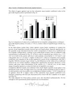
Before one can analyze the mass transport in the lumen or shell side of a capillary or on the
two sides of a flat membrane, the outlet or inlet mass transfer rate at the membrane interface
should be determined. A schematic diagram of the physical model and coordinate system is
given in Fig. 2. The mass transfer rate depends strongly on the membrane properties, on the
catalyst activity and the mass transfer resistance between the flowing fluid phase and
membrane layer. This mass transfer rate should then be taken into account in the mass
balance equation for the flowing fluid (liquid or gas) phase, on both sides of membrane
reactor. This will be discussed in section 6.
Mass Transfer in Multiphase Systems and its Applications

680
The mass transport through a catalytic membrane layer can be diffusive (there is no
transmembrane pressure difference between the two sides of the membrane layer) or
diffusive+ convective transport. These two modes of flow will be discussed separately due
to its different mathematical treatments in order to get the transfer rate.

membrane
C
o
C
δ
o
β
o
β
δ
o
J
J
δ
x
y
C
δ
C
r

Fig. 2. Illustration of the mass transfer through a membrane reactor
The other important classification of the reactors that, as it was mentioned, the membrane
reactor can intrinsically catalytic or it is made catalytic by dispersed catalyst particles
distributed uniformly in the membrane matrix. In this latter case two types of mathematical
model can be used (Nagy, 2007), namely pseudo-homogeneous or heterogeneous models,
depending on the catalyst particle size. It was shown by Nagy (2007) if the size of catalyst
particles less than a micron, the simpler homogeneous model can be recommended, in other
wise, the heterogeneous model should be applied.
The differential mass balance equation can generally be given by the following equation for

the catalytic membrane layer with various geometries, perpendicular to the membrane
interface, applying cylindrical coordinate (Ferreira et al., 2001):

(
)
(
)
(1)
m
m
Dc
c
p
cc
DQ
rrr r dr t
υ
∂
∂
+
∂
∂∂
⎛⎞
+−−=
⎜⎟
∂
∂∂ ∂
⎝⎠
(1a)
where p denotes a geometrical factor with values of 0 for cylindrical coordinate and -1 for

rectangular membranes. The membrane concentration, C is given here in a unit of measure
of gmol/m
3
. This can be easily obtained by means of the usually applied in the e.g. g/g unit
of measure with the equation of C=wρ/M, where w concentration in kg/kg, ρ – membrane
density, kg/m
3
, M-molar weight, kg/mol. The most often recommended mass balance
equation (Marcano & Tsotsis, 2002), in dimensionless form, for membrane reactor is as
(R=r/R
o
; C=c/c
o
):

2
*
1
o
m
R
CC
Q
DXRRR
υ
∂∂∂
⎛⎞
=−
⎜⎟
∂∂∂

⎝⎠
(1b)
where Q
*
reaction term given in dimensionless form. The boundary conditions are as:
Mass Transfer through Catalytic Membrane Layer

681
C=1 at X=0, for all R (2a)

0
C
R
∂
=
∂
at R=0, for all X (2b)

dC
CD J
R
υ
−
=
∂
at R=1, for all X (2c)
The value of the mass transfer rate through the membrane, J will be shown in the next
sections under different conditions. From eq. 1, the mass balance equation is easy to get for
flat sheet membrane.
2.1 Diffusive mass transport with intrinsic catalytic layer or with fine catalytic

particles
In both cases the membrane matrix is regarded as a continuous phase for the mass transport.
Assumptions, made for expression of the differential mass balance equation to the catalytic
membrane layer, are:
• Reaction occurs at every position within the catalyst layer;
• Mass transport through the catalyst layer occurs by diffusion;
• The partitioning of the components (substrate, product) is taken into account (thus,
CH
m
=C
*
m
where C
*
m
denotes membrane concentration on the feed interface; see Fig. 2);
• The mass transport parameters (diffusion coefficient, partitioning coefficient) are
constant;
• The effect of the external mass transfer resistance should also be taken into account;
• The mass transport is steady-state and one-dimensional;
In case of dispersed catalyst particles they are uniformly distributed and they are very fine
particles with size less than 1 μm, i.e. they are nanometer sized particles. It is assumed that
catalyst particles are placed in every differential volume element of the membrane reactor.
The reactant firstly enters in the membrane layer and from that it enters into the catalyst
particles where the reaction of particles is porous as e.g. active carbon, zeolite (Vital et al.,
2001) occurs or it enters onto the particle interface and reacts [particle is nonporous as e.g.
metal cluster, (Vancelecom & Jacobs, 2000)]. Consequently, the mass transfer rate into the
catalyst particles has to be defined first. In this case, the whole amount of the reactant
transported in or on the catalyst particle will be reacted. Then this term should be placed
into the mass balance equation of the catalytic membrane layer as a source term. Thus, the

differential mass balance equation for intrinsic membrane and membrane with dispersed
nanosized particles differ only by their source term. The cylindrical effect can only be
significant when the thickness of a capillary membrane can be compared to the internal
radius of the capillary tube as it was shown by Nagy (2006). On the other hand, the
application of cylindrical coordinate hinders the analytical solution for first or zero-order
reactions as well. Thus, the basic equations will be shown here for plane interface and in the
section 5 an analytical approach will be presented for cylindrical tube as well.
2.1.1 Mass transfer accompanied by first-order reaction
Herewith first the reaction source term will be defined indifferent cases, namely in cases of
intrinsically catalytic membrane and membrane with dispersed catalytic particles and the
solution of the differential mass balance equation under different boundary conditions.
Mass Transfer in Multiphase Systems and its Applications

682
2.1.1.1 Reaction terms
Intrinsically catalytic membrane; this is well known in literature (
11
o
kcΦ= ):

2
11
o
QkcC C=≡Φ (3)
Catalyst with dispersed particles, reaction takes place inside of the porous particles; For catalytic
membrane with dispersed nanometer size particles, the mass transfer rate into the spherical
catalyst particle has to be defined. The internal specific mass transfer rate in spherical
particles, for steady-state conditions and when the mass transport accompanied by first-
order chemical reaction can be given as follows (Nagy & Moser, 1995):

pp
j
C
β
∗
= (4)
where

()
1
tanh
pp
p
p
p
DHa
R
Ha
β
⎛⎞
⎜⎟
=
−
⎜⎟
⎝⎠
(5a)
and
2
1
p

p
p
kR
Ha
D
=

The external mass transfer resistance, through the catalyst particle depends on the diffusion
boundary layer thickness, δ
p
. The value of δ
p
could be estimated from the distance of
particles from each other (Nagy & Moser, 1995). Namely, its value is limited by the
neighboring particles, thus, the value of β
p
will be slightly higher than that follows from the
well known equation of 2 /
o
pp
m
dD
β
= , where the value of δ
p
is supposed to be infinite.
Thus, one can obtain (Nagy et al., 1989):

2
o

mm
p
pp
DD
d
β
δ
=+ (5b)
where
2
p
p
hd
δ
−
=
From eqs 4 and 5 one can obtain for the mass transfer rate with the overall mass transfer
resistance:

11
oo
tot
o
p
p
C
jcCc
H
β
β

β
==
+
(6)
Mass Transfer through Catalytic Membrane Layer

683
Accordingly, the Φ value in eq. 3 can be expressed as follows (Nagy et al., 1989):


2
1
m
tot
ωδ
β
ε
Φ=
−
(7)

Reaction occurs on the interface of the catalytic particles (Nagy, 2007). It often might occur that
the chemical reaction takes place on the interface of the particles, e.g, in cases of metallic
clusters, the diffusion inside the dense particles is negligibly. Assuming the Henry’s
sorption isotherm of the reacting component onto the spherical catalytic surface (CH
f
=q
f
),
applying

/
ff
DdC dr k H C
=
boundary condition at the catalyst’s interface, at r=R
p
, the Φ
reaction modulus can be given according to eq. (7) with the following β
sum
value:


1
11
o
ff
p
kH
δ
β
β
=
+
(8)

where k
f
is the interface reaction rate constant. The above model is obviously a simplified
one.
2.1.1.2 Mass transfer rates

The differential mass balance equation for the reactant entering the catalytic membrane
layer is as follows in dimensionless form:


2
2
2
0
dC
C
dY
−
Φ= (9)
Solution of eq. 9 is well known:

YY
CTe Se
Φ
−Φ
=+
(10)

For the sake of generalization, in the boundary conditions you should take into account the
external mass transfer resistance on both sides of the membrane, though it should be noted
that the role of the
o
δ
β
will be gradually diminish with the increase of the reaction rate. At
the end of this subsection the limiting cases will also be briefly given. Thus:

Y=0
()
0
1
m
o
m
Y
DdC
C
dY
β
δ
=
−=− (11)
Y=1
()
1
m
oo
m
Y
DdC
CC
dY
δδ δ
β
δ
=
−=− (12)

The mass transfer rate on the upstream side of the membrane can be given as follows (Nagy,
2007):

(
)
1
oo
mm
JHcTC
δ
β
=−
(13)
Mass Transfer in Multiphase Systems and its Applications

684
with

2
2
1tanh
1tanh
o
mm
o
o
mm
o
mm
o

mm
m
oo o o
H
H
HH
δ
δδ
β
β
ββ
β
β
ββ β β
⎛⎞
Φ
+Φ
⎜⎟
⎜⎟
⎝⎠
=Φ
⎛⎞
⎡⎤
Φ
⎛⎞
⎜⎟
⎣⎦
+Φ+Φ+
⎜⎟
⎜⎟

⎜⎟
⎜⎟⎝⎠
⎝⎠
(14)
and

1
tanh
cosh 1
o
mm
o
T
H
δ
β
β
=
⎛⎞
Φ
Φ
Φ+
⎜⎟
⎜⎟
⎝⎠
(15)
with
o
L
L

D
β
δ
=
;
o
m
m
m
D
β
δ
=

Similarly, the mass transfer rate for the downstream side of the membrane, at Y=1:

1cosh tanh
o
oo
mm
m
o
H
JHc C
δ
δδ
β
β
β
⎛⎞

Φ
=−ΦΦ+
⎜⎟
⎜⎟
⎝⎠
(14)
with

()
2
2
1
cosh
tanh 1
o
m
o
m
o
mm
mm
oo o o
HH
H
δ
δδ
β
β
β
β

ββ β β
Φ
=
Φ
⎛⎞
Φ
⎛⎞
⎜⎟
Φ
+++Φ
⎜⎟
⎜⎟
⎜⎟
⎝⎠
⎜⎟
⎝⎠
(15)
Limiting cases; The transfer rate without external mass transfer resistances, namely when
o
β
→∞and
o
δ
β
→∞, can easily be obtained from eq. 13 as limiting case as:

1
tanh cosh
oo o
m

cC
J
δ
β
⎛⎞
Φ
=−
⎜⎟
⎜⎟
Φ
Φ
⎝⎠
(16)
Eq. 16 is a well known mass transfer equation for liquid mass transfer accompanied by first-
order reaction. The mass transfer can similarly be obtained rate for the case when the outlet
concentration is zero, and,
o
δ
β
→∞:

oo
tot
J
c
β
=
(17)
where

00
1
tanh 1
o
tot
mm
H
β
β
β
=
Φ
+
Φ
(18)
Mass Transfer through Catalytic Membrane Layer

685
To avoid the outlet flow of reactant is an important requirement for the membrane reactors.
For it the operating conditions should be chosen rightly.
2.1.2 Mass transfer accompanied by zero-order reaction
In this case the reaction rate is independent of the concentration of reactant in the membrane
layer. The differential mass balance equation can be given as:

2
2
2
dC
dY
=

Φ
(19)
The value of Φ can be given for intrinsically catalytic membrane as:

2
0 m
o
m
k
Dc
δ
Φ=
(20)

C
A
o
i
δ
m
C
B
o
C
Aδ
o
C
Bδ
o
C

Bi
C
Ai

Fig. 3. Illustration of the concentrations for second-order reaction
The case of dispersed catalyst particles in the membrane layer is not discussed here because
it unimportance for membrane reactor. For the solution of the eq. 19 let us use the following
boundary conditions:
at Y=0
()
0
1
m
o
m
Y
DdC
C
dY
β
δ
=
−=− (21)
at Y=1
o
CHC
δ
=

(22)

The mass transfer resistance on the outlet side has not importance in that case because the
concentration rapidly decreases down to zero, thus does exist outlet mass transfer in a
Mass Transfer in Multiphase Systems and its Applications

686
narrow reaction rate regime, only. After solution, the concentration distribution can be given
as:

2
2
o
m
J
CY B
β
Φ
=
++
(23)
where

()
2
/2 /
1/
ooo
m
oo
m
C

B
H
δ
β
β
ββ
−Φ +
=
+
(24)
The mass transfer rate can be given as:

2
/2
/
o
oo
m
oo
m
HHC
Jc
H
δ
β
ββ
⎛⎞
−+Φ
⎜⎟
=

⎜⎟
+
⎝⎠
(25)
From eq. 25, the well known expression of mass transfer rate without chemical reaction can
easily be obtained.
2.1.3. Mass transfer accompanied by second-order reaction
It is assumed that the reagents (component A and B) are fed on the both sides of the
membrane reactor and they are diffusing through the membrane layer counter-currently
(Fig. 3). The reaction term can be given for intrinsically catalytic membrane as follows:

2
oo
AB A B
QkccCC=
(26)
Substituting the reaction term into eq. (1) for e.g. the A component and plane interface as
well as steady-state condition (D
mA
is constant) one can get:

2
2
2
0
oo
A
mA A B A B
dC
DkccCC

dy
−
=
(27)
This equation can be solved either by numerical method or an analytical approach can be
developed. Such an analytical approach is given in details in Appendix. The essential of this
method that the membrane layer is divided into N very thin sub-layer and the concentration
of one of the two components is considered to be constant in this sub-layer (see Fig. 3 and
Fig. 13). Thus, one can get a second-order differential equation with linear source term that
can be solved analytically. In dimensionless form it is for the ith sub-layer as:

2
2
2
0
A
Ai A
dC
C
dY
−
Φ=
for
1ii
YYY
−
≤
≤ (28)
where
2

2
oo
mAB B
Ai
mA
kccC
D
δ
Φ=
Mass Transfer through Catalytic Membrane Layer

687
where
B
C
denotes the average concentration of B component in the i
th
sub-layer. Solution of
eq. 28 is well known (see eq. 10). The general solution for every sub-layer has two
parameters that should be determined by the suitable boundary conditions (see Appendix):

at Y=0 C=1 (29)
at
1ii
YYY
−
≤≤
ii
AA
YY

dC dC
dY dY
−
+
=
with i=1,2,…,N (30)
at
1ii
YYY
−
≤≤
ii
A
YAY
CC
−
+
=
with i=1,2,…,N (31)
at y=1
o
A
A
CC
δ
= (32)
After solution of the N differential equation with 2N parameters to be determined the T
1

and S

1
parameters for the first sub-layer can be obtained as (ΔY is the thickness of the sub-
layers) :

()
()
1
1
2
1
2cosh
cosh
o
T
A
N
ON
NA
Ai
i
C
T
Y
Y
δ
ξ
ξ
=
⎛⎞
⎜⎟

⎜⎟
=− −
⎜⎟
ΦΔ
ΦΔ
⎜⎟
⎜⎟
⎝⎠
∏
(33)
and

()
()
1
1
2
1
2cosh
cosh
o
S
A
N
ON
NA
Ai
i
C
S

Y
Y
δ
ξ
ξ
=
⎛⎞
⎜⎟
⎜⎟
=−
⎜⎟
ΦΔ
ΦΔ
⎜⎟
⎜⎟
⎝⎠
∏
(34)
Knowing the T
1
and S
1
the other parameters, namely T
i
and S
i
(i=2,3,…,N) can be easily be
calculated by means of the internal boundary conditions given by eqs. 30 and 31 from
starting from T
2

and S
2
up to T
N
and S
N
.
After differentiating eq. 10 and applying it for the first sub-layer, the mass transfer rate of
component A can be expressed as:

()
()
()
1
1
2
1
2cosh
cosh
oST o
mAA N N A
ON
ST
m
NA
NN Aj
j
Dc C
J
Y

Y
δ
ξξ
δ
ξ
ξξ
=
⎛⎞
⎜⎟
Φ−
⎜⎟
=−
⎜⎟
ΦΔ
⎜⎟
−ΦΔ
⎜⎟
⎝⎠
∏
(35)
where

(
)
11
tanh
jj j
Ai
ii i
i

Y
z
ξξ κ
−−
ΦΔ
=+
for i=2,3,…,N and j=S,T,O (36)
Mass Transfer in Multiphase Systems and its Applications

688
and

()
1
1
tanh
j
jj
i
Ai
ii
i
Y
z
κ
κξ
−
−
=ΦΔ+ for i=2,3,…,N and j=S,T,O (37)
The starting values of

1
j
ξ
and
1
j
κ
are as follows:
1
1
A
Y
T
e
ξ
−
ΦΔ
=
1
1
A
Y
S
e
ξ
Φ
Δ
=
(
)

11
tanh
O
A
Y
ξ
=
ΦΔ
and
1
1
A
Y
T
e
κ
−
ΦΔ
=−
1
1
A
Y
S
e
κ
Φ
Δ
=
1

1
O
κ
=

Obviously, in order to get the inlet mass transfer rate of component A, the concentration
distribution of component B is needed. Thus, for prediction of the J value the concentration
of component B has to be known. It is easy to learn that trial-error method should be used to
get alternately the component concentrations. Steps of calculation of concentration of both
components can be as follows:
1.
Starting concentration distribution, e.g. for component B should be given and one
calculates the concentration distribution of component A;
2.
The indices of sub-layer of A component have to be changed adjusted them to that of B

started from the permeate side of membrane, i.e. at Y=1, thus, i subscript of A
i
should
be replaced by N+1-i;
3.
Now applying the previously calculated averaged A
i
(
i
A ), one can predict the
concentration distribution of component B, using eqs. 33 to 37, adapted them to
component B;
4.
These three steps should be repeated until concentrations do not change anymore;

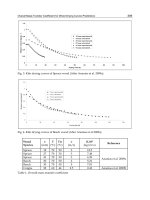
Fig. 4. The mass transfer rate a s a function of the catalyst phase holdup obtained by the
pseudo-homogeneous model (H
m
=H=1; D
m
=1 x 10
-10
m
2
/s;
0
o
C
δ
=
;
oo
δ
ββ
=
→∞
; d
p
=2 μm;
δ
m
=30 μm)
Mass Transfer through Catalytic Membrane Layer

689
2.1.4 Analysis of the mass transport
The detailed discussion of the mass transport through a membrane reactor is not a target of
this paper. Applying the equations for mass transfer rate or for concentration distribution
presented the reactor performance is easy to calculate. Only a typical figure will be shown in
this section. Fig. 4 illustrates the effect of the catalyst holdup and the reaction modulus on
the mass transfer rate. Detailed analysis is given in Nagy’s paper (2007). Similar results can
be obtained by zero-order reaction though its effect is somewhat stronger because its
independency of concentration (Nagy, 2007). The concentration of the reactor rapidly
decreases down to zero even at rather low reaction rate coefficient. Thus the role of the
convective velocity should have got careful attention.
Normally, 3-5 recalculations of concentrations are enough to get the correct results.
2.2 Diffuive+convective mass transport with intrinsic catalytic layer or with fine
catalytic particles
Convective mass transport can take place if transmembrane pressure difference exists
between the two membrane sides. Recently it was proved in the literature (Ilinitch, 2000,
Nagy, 2007) that the presence of convective flow can improve the efficiency of the
membrane reactor. Thus, the study of the mass transport in presence of convective mass
flow can be important in order to predict the reaction process. On the otherwise, the use of
convective flow is rather rare, because the aim is mostly to minimize the outlet rate of the
reactant on the permeate side. The source terms of this case are the same as it was showed in
subsection 2.1.
2.2.1 Mass transport accompanied by first-order reaction
The differential mass balance equation for the polymeric or macroporous ceramic catalytic
membrane layer, for steady-state, taking both diffusive and convective flow into account,
can be given as:

2
2

2
0
m
dC dC
Pe C
dY
dY
−
−Φ = (38)
where
m
m
m
Pe
D
υ
δ
=
;
()
2
1
m
tot
m
D
ωδ
β
ε
Φ=

−

where
υ denotes the convective velocity, D
m
is the diffusion coefficient of the membrane,
and δ
m
is the membrane thickness.

/2
m
Pe Y
CCe
−
=

(39)
Introducing a new variable,
C

(eq. 39) the following differential equation is obtained from
eq. 38):

2
2
2
0
dC
C

dY
−
Θ=


(40)
where
Mass Transfer in Multiphase Systems and its Applications

690
2
2
4
m
Pe
Θ
=+Φ

The general solution of eq. 40 is well known, so the concentration distribution in the
catalytic membrane layer can be given as follows:

YY
CTe Se
λ
λ
=+

(41)
with
2

m
Pe
λ
=
−Θ


2
m
Pe
λ
=
+Θ

The inlet and the outlet mass transfer rate can easily be expressed by means of eq. (41). The
overall inlet mass transfer rate, namely the sum of the diffusive and convective mass
transfer rates, is given by:

()
0
0
o
m
m
Y
m
Y
D
dC
JC TS

dY
υ
βλ λ
δ
=
=
=− =+

(42)
The outlet mass transfer rate is obtained in a similar way to eq. (42) for X=1:

(
)
o
m
JTeSe
λ
λ
δ
βλ λ
=+


(43)

C
°
C
δ
°

β
°
β
m
°
β
δ
°
catalyst particles
C
°
C
δ

(A) (B)
Fig. 5. Illustration of the concentration distribution for models A and B.
The value of parameters T and S can be determined from the boundary conditions. For the
sake of generality, two models, namely model A and model B, will be distinguished
according to Figure 5 (for details see Nagy, 2010). The essential difference between the
models is that, in case of model A, there is a sweeping phase that can remove the
transported component from the downstream side providing the low concentration of the
reacted component in the outlet phase and due to it, high diffusive mass transfer rate. There
Mass Transfer through Catalytic Membrane Layer

691
is no sweep phase in case of model B, thus the outlet phase is moving from the membrane
due to the lower pressure on the permeate side.
Model A. In this case, due to the effect of the sweeping phase, the external mass transfer
resistance on both sides of the membrane should be taken into account in the boundary
conditions, though the role of

o
δ
β
is gradually diminished as the catalytic reaction rate
increases. The concentration distribution in the catalytic membrane when applying a sweep
phase on the two sides of the membrane, as well is illustrated in Fig. 5a. On the upper part
of the catalytic membrane layer, in Fig. 5a, the fine catalyst particles are illustrated with
black dots. It is assumed that these particles are homogeneously distributed in the
membrane matrix. Due to sweeping phase, the concentration of the bulk phase on the
permeate side may be lower than that on the membrane interface. The boundary conditions
can be given for that case as:

(
)
oo
CCCJ
υβ
+
−= at Y=0 (44)

(
)
oo
CCCJ
δ
δδ δ δ
υβ
+
−= at Y=1 (45)
Boundary conditions given by eqs. (44) and (45) are only valid in two phase flows. Where

o
C
δ
denotes the concentration on the downstream side,
o
β
and
o
δ
β
are mass transfer
coefficients in the continuous phase,
o
m
β
the membrane mass transfer coefficient
(
/
o
mmm
D
β
δ
=
), H
m
denotes the distribution coefficient between the continuous phase and
the membrane phase. The solution of the algebraic equations obtained, applying eqs. 42 to
45, can be received by means of known mathematical manipulations. Thus, the values of T
and S obtained are as follows:

24
23 14
1
oooo
o
m
CC
T
δδ
βϕ βϕ
ϕϕ ϕϕ
β
−
=−
−
(46)
and

13
23 14
1
oo oo
o
m
CC
S
δδ
βϕ βϕ
ϕϕ ϕϕ

β
+
=
−
(47)
where
1
o
m
o
m
mm
Pe
e
H
H
λ
δ
β
ϕλ
β
⎛⎞
=+ −
⎜⎟
⎜⎟
⎝⎠

;
2
o

m
o
m
mm
Pe
e
H
H
λ
δ
β
ϕλ
β
⎛⎞
=+ −
⎜⎟
⎜⎟
⎝⎠

;
3
o
m
o
m
mm
Pe
H
H
β

ϕ
λ
β
=
−−

;
4
o
m
o
m
mm
Pe
H
H
β
ϕ
λ
β
=
−−;
An important limiting case should also be mentioned, namely the case when the external
diffusive mass transfer resistances on both sides of membrane can be neglected, i.e. when
o
β
→∞and
o
δ
β

→∞. For that case the concentration distribution and the inlet mass transfer
rate can be expressed by eqs. 48 and 49, respectively.
Mass Transfer in Multiphase Systems and its Applications

692

(
)
() ()
{}
1/2
/2
sinh 1 sinh
sinh
m
m
Pe Y
Pe
oo
m
e
CHCe YCY
δ
−
=⎡Θ−⎤+Θ
⎣⎦
Θ
(48)

[]

/2
sinh / 2 cosh
m
oo
m
Pe
m
JC C
ePe
δ
β
⎛⎞
Θ
=−
⎜⎟
⎜⎟
Θ+Θ Θ
⎝⎠
(49)
with
()
tanh /2
tanh
o
mm m
m
HPe
β
β
Θ

+Θ
=
Θ

An important limiting case when the outlet concentration is zero, i.e. 0
o
C
δ
=
, accordingly
the mass transfer rate is as
(
o
δ
β
→∞):

()
()( )
22
2
11
oo
o
m
o
m
c
J
Pe e e

β
β
λ
λ
β
−Θ −Θ
Θ
=
−
−− −

(50)
Model B. For the convective flow catalytic membrane reactor operating in another mode, for
instance in dead-end mode as in Figure 4b, the boundary condition on the permeate side of
the membrane should be changed. In this case the concentration of the permeate phase does
not change during its transport from the membrane interface. If there is no sweeping phase
on the downstream side then the correct boundary conditions will be as:

(
)
oo
CCCJ
υβ
+
−= at Y=0 (51)

CJ
δ
δ
υ

=
at Y=1 (52)
After solution one can get as:

12
23 14
1
oo
o
m
C
T
βϕ
ϕϕ ϕϕ
β
=−
−
(53)

1
23 14
1
oo
o
m
C
S
βϕ
ϕϕ ϕϕ
β

=
−
(54)
where
1
m
m
Pe
e
H
λ
ϕλ
⎛⎞
=−
⎜⎟
⎝⎠


2
m
m
Pe
e
H
λ
ϕλ
⎛⎞
=−
⎜⎟
⎝⎠



The values of φ
3
and φ
4
are the same as they are given after eq. 47.
2.2.2 Mass transport accompanied by zero-order reaction
The effect of the zero-order reaction will be discussed here for intrinsically catalytic
membrane layer, only. This reaction has no important role in the case of membrane reactor.
Mass Transfer through Catalytic Membrane Layer

693
The differential mass balance equation to be solved is as:

2
0
2
0
m
dC dC
Dk
dy
dy
υ
−
−= (55)
Similarly to eqs. 19, the differential mass balance equation for the catalytic membrane can be
given as:

2
2
2
m
dC dC
Pe
dY
dY
−
=Φ (56)
where
2
0
m
o
m
k
Dc
δ
Φ=

Look at first the solution with the following boundary conditions:
Y=0 then C=1 (57a)
Y=1 then
o
CC
δ
= (57b)
The general solution of Eq. (56) is as:

2
m
Pe Y
mm
m
CTe YQ
Pe
Φ
=−+
(58)
Applying the boundary conditions [Eqs. (57a) and (57b] one can get:

()
()
/2
/2
sinh 1 sinh
sinh /2 2 2
m
m
Pe Y
Pe
mm
b
p
m
Pe Pe Y
e
CCYSe C
Pe

−
⎧
⎫
⎛⎞
⎪
⎪
⎡⎤ ⎛⎞
=−++
⎨
⎬
⎜⎟
⎜⎟
⎢⎥
⎣⎦ ⎝⎠
⎪
⎪
⎝⎠
⎩⎭
(59)
The mass transfer rate can be given as:

(
)
1
oo
m
JcTC
δ
β
=− (60)

where
2
2
1
oo
mm
m
c
Pe
ββ
⎛⎞
Φ
=+
⎜⎟
⎜⎟
⎝⎠
;
22
1/
m
Pe
m
e
T
Pe
−
=
+Φ

The outlet mass transfer rate should also be given:

1
m
Pe
oo o
m
e
JcC
δδ δ
δ
βα
α
−
⎛⎞
=−
⎜⎟
⎜⎟
⎝⎠
(61)
where