Volume 18 - Friction, Lubrication, and Wear Technology Part 12 ppt
Bạn đang xem bản rút gọn của tài liệu. Xem và tải ngay bản đầy đủ của tài liệu tại đây (1.75 MB, 80 trang )
Fig. 27 Time-of-flight data for species composing the 1.9 eV ESDIED peak
Fig. 28 Time-of-flight data for species composing the 3.5 eV ESDIED peak
It has been shown (Ref 55) that the time-of-flight of an ion is proportional to its mass. The relationship is time-of-flight =
4.2 , where m is the mass of the ion. Hence, flight times of 4.2, 16.4, and 16.9 s are expected for H
+
, O
+
, and OH
+
,
respectively. Time-of-flight data for the 3.5 eV ESDIED peak also shows that H
+
is being desorbed, but that O
+
and/or
OH
+
are probably not.
ESD Applications. The data acquired for the polycrystalline tin oxide sample discussed in the previous section is
discussed further here. Consider the ESDIED and time-of-flight data shown in Fig. 29. The data were acquired after
annealing for 30 min at 600 °C (1110 °F) and 9.3 × 10
-7
Pa (7.0 × 10
-9
torr). Note that the 1.9 eV ESDIED peak is very
small relative to the higher-energy peak around 4.3 eV. The time-of-flight data of Fig. 30 and 31 show that O
+
and OH
+
are both desorbed, and the 4.3 eV peak has more O
+
than OH
+
, relative to the 1.9 eV peak.
Fig. 29 ESDIED spect
rum for polycrystalline tin oxide sample following annealing in vacuum for 30 min at 600
°C (1110 °F)
Fig. 30 Time-of-flight
data for species composing the 1.9 eV ESDIED peak following annealing in vacuum for 30
min at 600 °C (1110 °F).
Fig. 31 Time-of-
flight data for species composing the 4.3 eV ESDIED peak following annealing in vacuum for 30
min at 600 °C (1110 °F)
The ESD data can be explained by the following considerations. First, it is necessary to realize that tin oxide undergoes
dehydration for the annealing conditions used. This has been shown by Cox (Ref 57) using valence band ESCA. If it is
noted that the O
+
and OH
+
desorption signal is very small prior to annealing, but significantly larger following annealing,
it is clear that the surface O
+
and OH
+
for the clean sample, prior to annealing, are not active with regard to desorption by
electron stimulation. However, the O
+
and OH
+
that remain after dehydration are amenable to desorption by electron
stimulation. Therefore, oxygen and hydrogen not associated with water of hydration have been distinguished because
these bonding states are active with respect to ESD, whereas those associated with water of hydration are not.
It is possible to test this interpretation by exposing the sample to an oxidizing atmosphere. This was accomplished by
annealing the sample in oxygen for 1.5 h at 400 °C (750 °F) at 1.3 × 10
-4
Pa (10
-6
torr.) The ESDIED and time-of-flight
data are shown in Fig. 32 33 34. The 1.9 eV ESDIED peak has increased in size relative to that observed for the previous
600 °C (1110 °F) annealing treatment. The relative amounts of O
+
and OH
+
being desorbed have also decreased again,
compared with data collected following the 600 °C (1110 °F) annealing treatment.
Fig. 32
ESDIED spectrum for polycrystalline tin oxide sample following annealing in oxygen for 90 min at 400
°C (750 °F)
Fig. 33 Time-of-
flight data for species composing the 4.3 eV ESDIED peak following annealing in oxygen for 90
min at 400 °C (750 °F)
Fig. 34 Time-of-
flight data for species composing the 4.3 eV ESDIED peak following annealing in oxygen for 90
min at 400 °C (750 °F)
It is reasonable to expect oxygen supplied to the sample during the oxidation treatment to become associated with
vacancies generated during the dehydration process. Therefore, it can be concluded that the 1.9 eV ESDIED peak is
associated with water of hydration, and the higher-energy ESDIED peak is associated with other species, such as oxygen
bound to tin, in the lattice structure.
Thus, oxygen and hydroxyl groups associated with water of hydration are not active with regard to desorption by electron
stimulation, relative to oxygen and hydroxyl groups associated with other bonding situations. ESD has been used to
distinguish these oxygen and hydrogen types.
ESD is a valuable technique because it enables hydrogen detection and it can be used with minimum modifications to
existing AES equipment. The major drawback is that data interpretation beyond identification of desorbing species is
often difficult. An alternative to ESD is discussed next.
Secondary Ion Mass Spectrometry (SIMS)
SIMS is an analytical technique that has become very popular over the past few years. Enhanced element sensitivity and
hydrogen detection capability (order of ppm) are two advantages of SIMS that AES and XPS techniques do not offer. Its
primary disadvantages are that it is inherently a destructive technique and quantitation is more difficult, relative to
techniques such as AES and XPS.
Specific examples of the application of SIMS to studies of wear, lubrication, and friction are somewhat limited, when
compared with techniques such as AES. An excellent example of the application of SIMS to study material transfer
resulting from abrasive contact between a ceramic and several metals is described in Ref 58. SIMS is particularly suited
to such studies if the amounts of material transferred are expected to be very small.
SIMS Fundamentals. The SIMS process is performed by bombarding the surface of a solid target material of interest
with a beam of energetic ions. The ions composing the bombarding beam are referred to as primary ions. These ions can
be delivered to the target surface at energies up to approximately 40 keV. The result of collision processes between
primary ions and the target surface of interest is the emission of negative, positive, and neutral species. The term
"species" is employed to indicate that ions or agglomerations of atoms bearing a net charge can be emitted from the
surface. The species emitted from the surface are analyzed in terms of their mass-to-charge ratios (m/e). Therefore, only
charged species can be analyzed. Neutral species that have been sputtered from the surface must first be ionized before
analysis is possible.
It is important to point out that charged species leaving the target surface as a result of sputtering constitute only a small
portion of all sputtered atoms leaving the surface. This typically ranges from a few hundredths of a percent, up to
approximately 1%. Discussions of analytical descriptions of secondary ion yield and parameters that influence the overall
yield, such as ionization probability, are discussed in Ref 46 and 47.
SIMS can be performed in two modes. In one case, the primary ion beam is rastered over the surface covering an area of
approximately 50 × 50 m (2 × 2 mils) (Ref 46). This mode of analysis is referred to as static SIMS and is characterized
by a relatively slow removal rate of atoms from the surface of the target material.
Alternatively, the primary ion beam can be focused on an area of submicron dimension and material removed at very high
rates relative to static SIMS. This mode of operation is referred to as dynamic SIMS. Its sampling depth is on the order of
10
3
nm, whereas static SIMS is characterized by sampling depths of only a couple of atomic layers (Ref 46).
SIMS is often employed to obtain chemical depth profile information. Dynamic SIMS can achieve practical sputter rates,
as well as maximum sensitivity (Ref 46). Therefore, this section focuses on this mode.
In most cases, the primary ion beam employed with SIMS is an inert gas. However, primary beam systems should be
capable of generating both negatively and positively charged ions of reactive gases. Negatively charged ions, such as O
-
,
can be used as a primary beam source when sample charging is expected to be a problem. With versatility in the primary
beam source, electrically insulating materials can be analyzed with a minimum of difficulties.
An additional advantage of the ability to implement several types of primary ion beam gases is the effect of secondary ion
yield. This is because secondary ion yields are influenced by the charge characteristics at the surface. Ion yields are
maximized when neutralization probabilities are low. Therefore, positively charged secondary species are less likely to be
neutralized when electronegative atoms are present in surface and near-surface regions of the material from which
secondary ions are being sputtered. For this reason, if oxygen is used as a primary beam source, rather than an inert gas,
the emission of positively charged secondary ions can be expected to be enhanced. This point is discussed in Ref 47.
The SIMS spectrum consists of a representation of the signal intensity, or count rate, as a function of mass-to-charge
ratio (m/e). Consider the SIMS data presented in Fig. 35. These data represent a SIMS survey scan for the surface and
near-surface regions of a BiO
x
-Au-glass thin-film system, such as that discussed in the AES section (see Fig. 17). The
SIMS data in Fig. 35 contain several elements that do not appear in the film data in Fig. 17 (that is, elements in addition to
Bi, O, Au, and Si). These additional elements are the result of trace contamination of the deposition chamber from
previous deposition processes. This is an excellent example of the increased sensitivity of SIMS relative to AES.
Fig. 35 SIMS survey of bismuth layer of BiO
x
-Au-glass specimen
The reader should be aware that quantitation of SIMS data is a very complicated issue. The basis problem is the fact that
the secondary ion yield can be significantly influenced by several phenomena that can be very complex in nature. The
emission of secondary ions depends on the chemical and physical characteristics of the target surface, the primary beam
characteristics, and the matrix characteristics of the target material.
The most direct method of quantitation is to compare SIMS results with a reference material of known composition for a
given set of conditions for data acquisition. Of course, this involves the availability of reference materials for all
anticipated matrix configurations that might be encountered. At best, this is inconvenient. It would therefore be helpful if
a myriad of matrix configurations could be evaluated by simply extending data required for a minimum number of
reference samples.
In principle, this could be accomplished by the ability to extend relative sensitivity factors obtained for a few reference
materials to any arbitrary matrix configuration. This has been achieved by defining a parameter that characterizes the
electronic properties of the surface of the target material (Ref 59).
It is of interest to note that data from internal standards have been employed to specify parameters of a model to predict
relative atomic fraction values from secondary ion intensities (Ref 60). The model referenced here has been applied with a
reasonable degree of success when one considers that it has been applied to a variety of materials.
SIMS equipment includes an ion source (ion gun), a UHV environment, and a detection system that consists of
components such that energy and mass selection of the sputtered species occurs prior to the detector. References 47 and
59 provide a more detailed equipment description.
SIMS Applications. As previously mentioned, SIMS is a valuable technique in terms of detecting elements present in
relatively small concentrations, as well as detecting hydrogen. These capabilities can be particularly useful in friction,
lubrication, and wear problems involving materials that contain hydrogen and/or where small amounts of material transfer
occur.
Material transfer examples include that which results when materials are in tribocontact and that which results from
diffusion processes. Material transfer by diffusion is often difficult to substantiate, especially if the amount of mass
transfer is relatively small.
For the purpose of demonstration, the interdiffusion of constituents composing a layered BiO
x
-Al-glass system is
discussed. This system is analogous to the BiO
x
-Au-glass thin-film system previously discussed and is used here because
the amount of interdiffusion associated with high-temperature oxidation of the BiAl-glass-layered structure is substantial
and can be clearly identified.
Consider the SIMS depth profile data shown in Fig. 36 and 37. These data respectively represent results for a layered
structure that was not subjected to high-temperature oxidation, and a layered structure that was. The secondary ions
monitored are Al
+
, Bi
+
, O
+
, and Si
+
. The data clearly demonstrate that interdiffusion occurs among constituents of the
bismuth layer, the metal layer, and the glass substrate. It is interesting to note that interdiffusion processes for this system
were, in general, not nearly as observable with AES depth profiling as with SIMS. Again, this demonstrates the advantage
of the increased sensitivity of SIMS, relative to other surface analytical techniques.
Fig. 36 SIMS depth profile of layered Bi-Au-glass specimen
Fig. 37 SIMS depth profile of layered BiO
x
-Au-glass specimen
It is important at this point to emphasize that care must be taken when evaluating data acquired near interfacial regions.
This consideration is often applicable when mass transport by diffusion is of interest. The important point is that the
sputtering process can produce mixing of constituents across the interface, which results in peak broadening in the
composition profile. Such broadening can be interpreted as diffusion effects if sufficient care is not taken. The most
practical way to avoid difficulty is to evaluate reference materials for comparison, as was done here by comparing a
sample not subjected to high-temperature oxidation to a sample that was.
The capability to detect hydrogen can be very useful in friction, lubrication, and wear studies because such studies often
involve systems that contain hydrogen. For instance, Sugita and Ueda (Ref 61) studied the wear characteristics of silicon
nitride in water with respect to the material produced at the specimen-counterface interface. SIMS analysis showed that
the worn surface contained silicon bonded to oxygen and hydrogen. Therefore, silicon was oxidized as a result of the
tribocontact. The presence of hydrogen suggests that the oxidized silicon is hydrated to some extent. X-ray diffraction
data were used in conjunction with the SIMS data to propose a mechanism of material removal for this system of silicon
nitride rubbing against silicon nitride in a water environment. The mechanism proposed is one in which the silicon in
silicon nitride is first oxidized and then converted to an amorphous form of silica hydrate, which is then removed by
frictional forces associated with the rubbing of the two silicon nitride faces.
Thus, SIMS provides a means by which hydrogen can be detected and a means by which elements can be observed at
very low concentrations. Its primary disadvantages are that it is inherently a destructive technique and chemical bonding
information such as that obtained with XPS and AES is not available.
Infrared (IR) Spectroscopy
The IR spectroscopy technique should be mentioned because it is becoming more important in the study of the chemistry
of solid surfaces; however, it will not be treated in detail in this article. Infrared spectroscopy has been employed for some
time as a routine technique for determining the molecular structure of organic compounds, and therefore it is not a new
technique.
IR spectroscopy is performed by subjecting the sample to a source of IR radiation. This source is sometimes referred to as
an emitter. For practical purposes, the IR range is taken to be electromagnetic radiation within the energy range for 200 to
4000/cm. In practice, more than one type of emitter is required to cover the entire IR range. The electric field of the
electromagnetic radiation can couple with oscillating dipoles of vibrating molecules. The result of this interaction, or
coupling, of the electromagnetic radiation with vibrational energy modes of molecules is absorption of the radiation.
The IR absorption spectrum appears in the form of the percent of radiation transmitted through the sample (that is, not
absorbed) as a function of IR radiation energy. Structures that are expected to be active with regard to IR absorption are
those that exhibit a net dipole moment. Symmetric molecules, such as N
2
and O
2
, are not expected to exhibit an
absorption species for any relative position of the atoms (bond length). On the other hand, molecules such as HCl, NO,
and CO are expected to exhibit characteristic absorption frequencies.
Problems in friction, lubrication, and wear can involve analysis of surface components that are present in coverages of
considerably less than one monolayer. This is possible with IR spectroscopy, but most investigators employ the technique
of multiple internal reflectance (MIR) spectroscopy for such studies. This technique offers increased sensitivity for
surface components, allowing detailed studies of adsorbate-surface interactions. In fact, MIR spectroscopy can be used to
determine the orientation of adsorbate molecules on solid surfaces. Both IR and MIR spectroscopy are discussed further
in Ref 62 and 63.
References
1. H. Hertz, Ann. Physik, Vol 31, 1887, p 983
2. J.J. Thompson, Phil. Mag., Vol 48, 1899, p 547
3. A. Einstein, Ann. Physik, Vol 17, 1905, p 132
4. K. Siegbahn, C. Nordling, G. Johansson, J. Hedman, R
F. Heden, K. Hamrin, U. Gelius, T. Bergmark, L.O.
Werme, R. Manne, and Y. Baier, ESCA Applied to Free Molecules, North-Holland, Amsterdam, 1969
5.
K. Siegbahn, C. Nordling, A. Fahlman, R. Nordberg, K. Hamrin, J. Hedman, G. Johansson, R. Bergmark,
S
E. Karlsson, I. Lindgren, and B. Lindberg, ESCA: Atomic, Molecular and Solid State Structures Studied
by Means of Electron Spectroscopy, Nova Acta Regiae Soc. Sci. Upsaliensis,
Ser. IV, Vol 20, Almquist and
Wiksells, Uppsala, 1967
6. T.A. Carlson, X-Ray photoelectron Spectroscopy,
T.A. Carlson, Ed., Dowden, Huntington & Ross, Inc.,
1978
7. K.W. Nebesny, B.L. Maschhoff, and N.R. Armstrong, Anal. Chem., Vol 61, 1989, p 469A
8. A.A. Galuska, J. Vac. Sci. Technol. B, Vol 8, 1990, p 488
9. S.D. Gardner, G.B. Hoflund, M.R. Davidson, and D.R. Schryer, J. Catalysis, Vol 115, 1989, p 132
10.
M.R. Davidson, G.B. Hoflund, L. Niinista, and H.A. Laitinen, J. Electroanal. Chem., Vol 228, 1987, p 471
11.
G.B. Hoflund, D.A. Asbury, S.J. Babb, A.L. Grogan, Jr., H.A. Laitinen, and S. Hoshino,
J. Vac. Sci,
Technol. A, Vol 4, 1986, p 26
12.
G.B. Hoflund, A.L. Grogan, Jr., D.A. Asbury, H.A. Laitinen, and S. Hoshino, Appl. Surf. Sci.,
Vol 28, 1987,
p 224
13.
G.B. Hoflund, M. Davidson, E. Yngvadottir, H.A. Laitinen, and S. Hoshino, Chem. Mater.,
Vol 1, 1989, p
625
14.
M.R. Davidson, G.B. Hoflund, and R.A. Outlaw, J. Vac. Sci. Technol. A, Vol 9, 1991, p 1344
15.
M. Cardona and L. Ley, Photoemission in Solids I: General Principles,
M. Cardona and L. Ley, Ed.,
Springer-Verlag, Berlin, 1978
16.
A. Azouz and D.M. Rowson, A Comparison of Techniques for Surface Analysis of Extreme Pre
ssure Films
Formed During Wear Tests, Microscopic Aspects of Adhesion and Lubrication,
J.M. Georges, Ed., Elsevier,
Amsterdam, 1982
17.
B.A. Baldwin, Lubr. Eng., Vol 32, 1976, p 125
18.
R.J. Bird, Wear, Vol 37, 1976, p 132
19.
G.B. Hoflund, H L. Yin, A
.L. Grogan, Jr., D.A. Asbury, H. Yoneyama, O. Ikeda, and H. Tamura,
Langmuir, Vol 4, 1988, p 346
20.
C.R. Brundle and A.D. Baker, Ed., Electron Spectroscopy: Theory, Techniques and Applications,
Academic
Press, 1977
21.
C.D. Wagner, W.M. Riggs, L.E. Davis, J.F. Moulder, and G.E. Muilenberg, Ed., Handbook of X-
Ray
Photoelectron Spectroscopy, Perkin-Elmer Corporation, 1979
22.
S. Hagstrom, C. Nordling, and K. Siegbahn, Z. Phys., Vol 178, 1964, p 439
23.
J.A. Gardella, Jr., Anal. Chem., Vol 61, 1989, p 589A
24.
D.M. Hercules, Anal. Chem., Vol 50, 1978, p 743A
25.
H. Fellner-Feldegg, U. Gelius, B. Wannberg, A.G. Nilsson, E. Basilier, and K. Siegbahn,
J. Electron
Spectrosc. Relat. Phenom., Vol 5, 1974, p 643
26.
P.W. Palmberg, J. Electron Spectrosc., Vol 5, 1974, p 691
27.
G.B. Hoflund, D.A. Asbury, C.F. Corallo, and G.R. Corallo, J. Vac. Sci. Technol., Vol 6, 1988, p 70
28.
H. Ferber, C.K. Mount, G.B. Hoflund, and S. Hoshino, Surface Studies of N Implanted and Annealed
ABCD Chromium Films, Thin Solid Films, Vol 203, 1991, p 121
29.
V.D. Castro and G. Polzonetti, J. Electron Spectrosc. Relat. Phenom., Vol 48, 1989, p 117
30.
D.P. Smith, Surf. Sci., Vol 25, 1971, p 171
31.
E.P.Th.M. Suurmeijer and A.L. Boers, Surf. Sci., Vol 43, 1973, p 309
32.
E. Taglauer and W. Heiland, Appl. Phys., Vol 9, 1976, p 261
33.
E. Taglauer and W. Heiland, Surf. Sci., Vol 33, 1972, p 27
34.
S.H.A. Bageman and A.L. Boers, Surf. Sci., Vol 30, 1972, p 134
35.
D.S. Karpuzov and V.E. Yurasova, Phys. Status Solidi (b), Vol 47, 1971, p 41
36.
R.F. Goff and D.P. Smith, J. Vac. Sci. Technol., Vol 7, 1970, p 72
37.
W. Heiland, H.G. Schäffler, and E. Taglauer, Surf. Sci., Vol 35, 1973, p 381
38.
X.Z. Jiang, T.F. Hayden, and J.A. Dumesic, J. Catalysis, Vol 83, 1983, p 168
39.
A.J. Simoens, R.T. Baker, D.J. Dwyer, C.R Lund, and R.J. Madon, J. Catalysis, Vol 86, 1984, p 359
40.
P.N. Belton, Y.M. Sun, and J.M. White, J. Phys. Chem., Vol 8, 1984, p 5172
41.
S.J. Tauster, S.C. Fung, and R.L. Gartner, J. Am. Chem. Soc., Vol 106, 1980, p 170
42.
H. Niehus and E. Bauer, Surf. Sci., Vol 47, 1975, p 222
43.
S.V. Pepper, J. Appl. Phys., Vol 45, 1974, p 2947
44.
N. Takahashi and K. Okador, Wear, Vol 38, 1976, p 177
45.
H.J. Mathien and D. Landolt, Wear, Vol 66, 1981, p 87
46.
D. Briggs and M.P. Seah, Practical Surface Analysis by Auger and X-Ray Photoelectron Spectroscopy,
John Wiley & Sons, 1983
47.
L.C. Feldman and J.W. Mayer, Fundamentals of Surface and Thin Film Analysis, North-Holland, 1986
48.
C. Kittel, Introduction to Solid State Physics, 5th ed., John Wiley & Sons, 1976
49.
L.E. Davis, N.C. MacDonald, P.W. Palmberg, G.E. Riach, and R.E. Weber,
Handbook of Auger Electron
Spectroscopy, Physical Electronics Industries, Inc., 1976
50.
G.B. Hoflund, A.L. Grogan, Jr., and D.A. Asbury, J. Catalysis, Vol 109, 1988, p 226
51.
A.L. Grogan, Jr., V.H. Desai, S.L. Rice, and F. Gray III, Apparatus for Chemomechanical Wear Studies
with Biaxial Load and Surface Charge Control, Wear, accepted for publication
52.
G.B. Hoflund, Scanning Electron Microsc., Vol IV, 1985, p 1391
53.
D. Menzel and Gomer, J. Chem. Phys., Vol 41, 1964, p 3311
54.
M.L. Knotek and P.J. Feibelman, Phys. Rev. Lett., Vol 40, 1978, p 964
55.
M.M. Traum and D.P. Woodruff, J. Vac. Sci. Technol. A, Vol 17, 1980, p 1203
56.
R.E. Gilbert, D.F. Cox, and G.B. Hoflund, Rev. Sci. Instrum., Vol 53, 1982, p 1281
57.
D.F. Cox, G.B. Hoflund, and H.A. Laitinen, Appl. Surf. Sci., Vol 20, 1984, p 30
58.
K. Fujiwara, Wear, Vol 51, 1978, p 127
59.
A.W. Czanderna, Methods of Surface Analysis,
Methods and Phenomena, Their Applications in Science
and Technology, Elsevier, Amsterdam, 1975
60.
C.A. Anderson and J.R. Hinthrone, Anal. Chem., Vol 45, 1973, p 1421
61.
T. Sugita and K. Ueda, Wear, Vol 97, 1984
62.
B.P. Straughan and S. Walton, Ed., Spectroscopy, Chapman and Hall, London, 1976
63.
N.J. Harrick, Internal Reflection Spectroscopy, Interscience, 1967
X-Ray Characterization of Surface Wear
C.R. Houska, Virginia Polytechnic Institute and State University
Introduction
X-RAY DIFFRACTION and spectroscopy provide a variable-depth probe of the atomic arrangements and composition of
near-surface material. Depending on the sample, x-ray wavelength, and experimental arrangement, quantitative data from
about 10 nm to a number of m can be provided. This range of penetration depth can be used to examine wear-modified
and unmodified regions. Deeper penetrations allow unmodified material to be sampled as a reference for those changes
taking place near the surface.
The first consideration is to examine the conditions that determine penetration depths for both x-ray diffraction (XRD)
and x-ray fluorescence (XRF). Both kinds of data can be obtained using either commercially available equipment or
specialized beamlines at synchrotron radiation facilities. Synchrotron beamlines allow more flexibility in the choice of
wavelengths and provide highly collimated and intense beams that add to the capability to alter the penetration distance
by adjusting the optical arrangement. Small glancing angles between the specimen surface and either the incident or
diffracted beams are effective in probing closer to the surface.
X-rays can become totally reflected from locally flat surfaces at extremely low angles of incidence (<0.25°). Under these
conditions, beam penetration becomes anomalous and limited to less than 8 nm. Penetration distance, , depends on
the angle of incidence,
i
, relative to the critical angle,
c
; that is,
(Eq 1)
where = x-ray wavelength (Ref 1).
An uncertainty or divergence in the angle of the incident beam,
i
, can introduce a large uncertainty in penetration
distance. A wavy or rough surface and an ideally parallel beam also leads to quantitative uncertainties because
i
takes on
a range of values. Because of these difficulties in determining penetration distance with total reflection, the subsequent
discussion involves glancing angles that are greater than the critical angle. Above the critical angle, one can define
penetration distances more simply using a large data file of absorption coefficients (Ref 2) and more conventional
equipment.
Surface roughness introduces an additional complication. Near the surface, signal-producing material is removed. Where
it exist, the beam paths differ from point to point at a fixed distance below the mean surface. A fluctuation in path length
produces a net decrease in the measured signal (Ref 3). This problem has been studied using severely ground samples and
a correction given in terms of a Gaussian distribution of asperities with correlation (Ref 4).
X-Ray Diffraction and Fluorescence from Flat Surfaces
Analyses of penetration distances are typically based on flat surfaces. The surface need only be flat over a distance that
allows the incident and outgoing signal beams to see a locally flat region of the surface. Under these conditions, beam
paths enter and leave near-surface material only once. Both diffraction and fluorescence signals are treated together with a
common absorption term. XRF has one more absorption term, because of a difference in the incident and fluorescence
wavelengths.
The following discussion refers to a differential element of irradiated area
(Eq 2)
and thickness, dZ. The various terms, along with the tilt angle, , are illustrated in Fig. 1. A
0
is the cross section of the
incident beam with incident angle, + , and intensity, I
0
. If the signal angle is - , the fluorescent signal from an
element at a depth, Z, is given by (Ref 5):
(Eq 3)
with
(Eq 4)
and
(Eq 5)
where N
i
= number of i atoms/volume,
i
= total atomic cross section of atom i, D
i
= dimensionless absorption factor for
fluorescent radiation in the path from sample surface to detector multiplied by the detector efficiency, and R = sample-to-
detector distance.
Fig. 1 X-ray optics illustrating:
i
= angle of incidence,
s
= signal angle,
= angle of tilt from symmetrical
arrangement, and 2 = angle between signal and incident beam. Other quantities include A
0
= cross-
sectional
area of incident beam, and total volume of signal element is A
0
/sin( + ) multiplied by its thickness, dZ,
located at a depth - Z. The detector is located at a distance R from the sample.
For a diffracting element, Q
D
differs, depending on whether the volume dV contains a single crystal or a polycrystalline
substance. Only a polycrystalline substance with a flat surface, which gives (Ref 6, 7)
(Eq 6)
will be considered. Here, is the Bragg angle for the sample, V
C
is the volume of the unit cell, ' is the Bragg angle of the
monochromator, if used, j is the multiplicity, and F is the structure factor. If the thermal factor is known, it can be
included as an additional term in Q
D
.
The exponential term in Eq 2 is of primary interest because it determines beam penetration. With a fluorescence signal,
two linear absorption coefficients are required; that is, one for the incident beam,
i
, and another for the signal as it leaves
the sample,
s
. For diffraction, the incident and signal wavelength are the same with
i
=
s
= . The absorption
coefficient depends on the material and wavelength.
With a homogeneous sample, the contributions from all layers are obtained by integrating Eq 3. One normally integrates
to infinity for a thick sample, giving the effective penetration distance.
Z
0
= (
i
S)
-1
(Eq 7)
where the path length factor is
(Eq 8)
The total signal for all elements becomes
(Eq 9)
which is written so as to isolate the effective volume term on the right. The term on the left is the reduced integrated
intensity, where P is determined by the total area under a peak.
If one considers a pair of rays entering and leaving the sample, penetrating to a distance equal to the effective penetration
distance, Z
0
, the beam is reduced by e
-1
purely from sample absorption. The accumulated signal from all elements
between the surface and Z
0
relative to an infinitely thick sample is 1 - e
-1
, or 0.63. As increases, the trend is for the
penetration distance to decrease as the absorption coefficient usually increases. However, crossing an absorption edge
causes a sudden change in the penetration distance (Ref 8). Another common way of decreasing the penetration distance
is to decrease the angle of incidence below the Bragg angle, , with a fixed 2 . This decreases S
-1
for a particular Bragg
peak as one goes toward smaller glancing angles. In fact, one can tilt the sample so that the glancing angle is one the
signal side and obtain a similar decrease. The direction of tilt does influence the area of beam as it intersects with the
sample and gives a higher effective volume at low angles of incidence and, therefore, more intensity.
Figure 2 illustrates changes in the effective penetration for a large in angles with CuK ( = 0.1542 nm), CrK ( =
0.2291 nm), a partially stabilized zirconia sample (PSZ), and the (111) and (400) Bragg reflections (Ref 9). A wavelength
of 0.4 nm is also shown with the (111) set to illustrate an extreme wavelength that is only available at a synchrotron
radiation beamline. Here, it can be seen that when the angle of incidence equals the signal angle, the effective penetration
is a maximum at 0.42 m, and can be further reduced to 0.02 m for ± tilts of 40°. This would give glancing angles
below 2.9° for a Bragg angle of 42.9°. In other words, 63% of the Bragg peak would come from the region between the
surface and 0.02 m. Changing from CrK to CuK , radiation increase the maximum penetration from 1.05 to 2.08
m.
Fig. 2
Examples of effective flat sample penetration depths for (111) and (400) peaks with various wavelengths
(0.4 nm, CrK ) and CuK and tilt angle
. All are based on the absorption in partially stabilized zirconia and
its lattice constant. The maximum tilt is limited by and the critical angle for total reflection.
One would have to go to even lower glancing angles to attain 0.02 m, which may not be practical with commercial x-ray
systems. The relatively high absorption coefficient of zirconia tends to give limited penetration. A similar family of
curves is found for the (400), but with larger penetration distance, because of the larger Bragg angle for the reflection .
At a larger , larger tilts are required to attain glancing angle conditions. This larger range in is visible when the
(111) family is compared with the (400).
X-Ray Diffraction and Fluorescence from Rough Surfaces
The Gaussian distribution is commonly used to describe the distribution of excursions (Ref 9, 10). It is also convenient to
use for x-ray problems. With this distribution, the density of excursions from the mean surface plane between locations Z
1
and Z
1
+ dZ
1
is
(Eq 10)
where is the standard deviation of the excursions.
The area fraction of sample at a distance Z
1
from the mean plane is
(Eq 11)
This is the well-known error function complement shown at the right of Fig. 3. It is 0.5 at the mean plane, 0 for large
positive excursions beyond about +2 , and 1 for those deeper than -2 into the sample.
Fig. 3 Location of signal-producing elements about the mean
plane of a surface with a Gaussian distribution of
asperities. Area fraction, A
f
, of occupied sampling plane is shown to right.
X-ray diffraction from polycrystalline samples requires that crystallites be oriented to satisfy Bragg's law. For
polycrystalline samples, this usually turns out to be a small fraction of the sampling plane, unless one is using an oriented
single crystal. Consequently, the statistical signal fluctuation from XRD can be large for material near the mean plane,
unless the material has very small grains. This is not the case for x-ray fluorescence analysis, where all atoms near the
surface have a finite probability to contribute a measurable signal.
With a real surface, the signal-producing elements are likely to be correlated with absorbing elements in either the
entrance path or along an exit path out of the sample. This surface roughness problem has been treated using numerical
calculations based on a Gaussian distribution with correlation (Ref 4). There is no simple analytical answer to this
problem. Some general conclusions allow one to establish conditions where surface roughness calculations become
unimportant. The x-ray theory contains a correlation parameter,
c
, which indicates how quickly a surface excursion loses
correlation with increasing distance, , from a neighboring point. A large
c
causes neighboring points along the surface
to look alike, whereas a small
c
causes nearby points to be unrelated.
An estimate for the value, giving the maximum integrated intensity correction for roughness, can be obtained from
(Eq 12)
Likewise, if one is not to exceed a maximum intensity correction of 15%, the following condition should be satisfied:
2.4
-1
(Eq 13)
The term 2.4 can be related directly to the full width at the half maximum of the Gaussian probability distribution. A
15% correction would represent routine work. For precision work, the maximum given by Eq 13 should be decreased
by one-half.
Equation 12 describes the condition of having the incident and signal beams oriented parallel to the mean slope of the
surface. This shifts the correction to low angles when the correlation parameter
C
becomes large, relative to . Both Eq
12 and 13 treat a sample having a statistically homogeneous distribution of signal elements. When strain gradients that are
present near the surface are as large or smaller than 2.4 , correlation between the signal elements and the exit and entry
paths should be considered for a quantitative treatment of the data.
The roughness correction has been shown to go to zero at the extremes of 90° and 0° under symmetrical
conditions (Ref 3). At these limits, the paths are either completely correlated or are uncorrelated. The statistical model
previously cited (Ref 4) does not treat the case when an incident or signal ray is likely to see more than one asperity.
Experience with the examination of rough surfaces using x-rays is very limited. At this time, x-rays do not appear to give
results as good as those obtained using profilometer data in order to determine the statistical parameters that describe real
surfaces. At low glancing angles, either with the incident or the signal beam, one can lose quantitative accuracy of
intensity data when Z
0
approaches the mean surface excursion distance. However, this need not be a problem for either
qualitative chemical or phase identification. Routine approaches for identification problems are described in Ref 8.
Near-Surface Gradients
Equation 2 defines the reduced intensity in terms of a thin slab element having an irradiated area A
e
= A
0
/sin( + ). For
a single-phase homogeneous material free of strain, all elements can be treated as identical and either summed or
integrated to obtain the full signal. This led to the integral result for the effective volume, Eq 9. If the surface has been
disturbed mechanically, thermally, or chemically, and this produces a change in the spacing of diffracting planes that
extends over those probe distances already discussed, the Bragg peaks become distributed over a range of 2 angles.
Peaks are no longer superimposed at the same position and can be treated as differential behavior. Both integral and
differential gradients have been described in terms of a continuous distribution function, H
i
(Z), which describes the
gradient of i with distance Z below the surface (Ref 11, 12). The subscript designates the kind of distribution; that is,
residual strain, atom type, a particular phase, texture, grain size, or other structural disturbances distributed along a
gradient. These can be defined as integral or differential gradients with respect to the signal elements, depending on
whether the intensity is unshifted or shifted in 2 .
A feature that exhibits a differential behavior displays a change in the d-spacing with position along the gradient zone.
Under these conditions, the diffraction angle 2 between the incident and signals beams changes according to Bragg's
law:
n = 2d(Z) sin (Z)
(Eq 14)
A change in d causes a distribution of intensity over a range in 2 angles. The most often leads to an asymmetrical
broadening of the Bragg peak, which can be produced by chemical or residual strain gradients. The intensity of the
diffracted signal is again proportional to the effective volume or the area of sampling plane multiplied by its thickness,
which is given by (Ref 13, 14):
(Eq 15)
This depends on the d-spacing gradient, dd/dZ, over each element and leads to a redistribution of the Bragg intensity,
along with 2 axis or differential behavior. Equation 15 indicates that a small d-spacing gradient tends to give higher
intensity.
A fluorescence signal "i" of a fixed wavelength at each position Z gives integral behavior over a gradient zone. When
analyzed by a crystal or energy-dispersive detector, one finds that signals at different depths with a common
superimpose. Therefore, the total signal is obtained by summing all measurable signals to some effective distance below
the surface. Here, the signal is not dispersed at each depth -Z. Integral behavior is expected from a gradient in the volume
fraction of crystal phases having fixed compositions. Here, the diffraction signals accumulate from the entire zone at fixed
2 positions, giving relatively sharp peaks. The positions are simply determined from Bragg's law and the published
lattice parameters and structures (Ref 8) of the various phases along a zone.
Texture can also be treated as an integral quantity because fixed lattice parameters produce an accumulation of diffracted
signals from all parts of a zone. If a texture gradient exists over the probe distance considered, the variation in relative
integrated intensity from one Bragg peak to another will vary, depending on the pole density gradient of the diffracting
planes and the probe depth. A severe thermal-mechanical disturbance at the surface could produce crystallite reorientation
and a measurable texture gradient. This problem has not been examined quantitatively.
A grain-size gradient in the range that produces x-ray diffraction line broadening (<100 nm) could give different line
widths, again, depending on the gradient, probe depth, and instrument resolution. Because each diffraction peak occurs at
the same 2 position from different portions of the zone, it is considered to be integral behavior. A similar argument can
be given for nonuniform strain, but without a uniform strain component. This might be produced by a gradient in the
dislocation density. At high dislocation densities, the diffraction peaks become broadened at fixed 2 positions. This
leads to an integral behavior, with either line width or shape changing with probe depth.
There are normally inherent differences in our ability to accurately detect changes in differential and integral
measurements. Conventional x-ray diffraction sources are typically of low intensity and require long counting times to
attain statistical accuracies better than 5% when polycrystalline samples are used. Integral behavior is examined largely
from changes in relative intensity measurements as they vary with different probe depths. Differential behavior further
depends on changes in the intensity distribution with 2 which is usually very sensitive to the gradient profile. The
accuracy of the 2 scale can easily be 1 in 10,000, making an XRD measurement of differential behavior highly accurate.
The following sections provide examples of both integral and differential behavior using XRD.
Integral Gradient
The examination of phase gradients along a wear track of a partially stabilized zirconia disk by XRD provides an example
of integral behavior. Three distinct crystal phases can be present in this material: cubic, tetragonal, and monoclinic.
Linear, exponential, and stepped distributions have been considered (Ref 11, 12). The exponential distribution can be
written as (Ref 11):
H
i
(Z) = H
0i
+
(Eq 16)
The various terms are illustrated and defined in the caption of Fig. 4. For each position Z, it is required that
H
i
(Z) = 1
(Eq 17)
where all phases i are considered. The effective volume for each phase is obtained by integration
(Eq 18)
with
(Eq 19)
and the subscript i refers to the Miller indices (hkl) reflecting at an angle . The linear absorption coefficient averaged
over all phases is < >. For the exponential distribution given by Eq 11, this simplified to
(Eq 20)
for a flat sample.
Fig. 4 Experimental near-surface area fraction distribution showing: undisturbed substrate limit, H
0i
; surface
area fraction, H
si
, and location e
-1
point in terms of -b
i
The quantity S is the path length factor given in Eq 8 with
s
=
i
. S becomes very large as ± . Two cases are
considered below.
In the first case, the beam samples only a small fraction of the exponential distribution. This condition requires that (b
i
<
>S) 1. A large value for any one of these terms could limit the overall view of the gradient. Therefore, it is reasonable
that the effective volume for phase i should be
(Eq 21)
That is, only the phase distributions at the surface are seen.
In the second case, if (b
i
< >S) 1, due to any one or any combination of these terms, the near-surface gradient is too
small to be observable. Therefore, the effective volume is determined by the volume fraction in the substrate
(Eq 22)
In order to evaluate b
i
, at least one measurement should be made in the range (b
i
< >S 1, and additional measurements
are required to solve for H
Oi
and H
si
. These are obtained at different values or with different values, because of a
change.
The determination of the phase distributions for a polished PSZ dish after a wear test was conducted for both the worn
track and an unworn region (Ref 11). The wear testing was conducted at an ambient temperature of 204 °C (400 °F), with
an atmosphere of prepurified nitrogen. A 6.4 mm (0.25 in.) diameter pin was loaded to 12.5 N (1.27 kgf) against a disk
traveling at 0.3 m/s (1 ft/s) at the point of contact. The total time of testing was 61 h. XRD patterns from both the worn
track and the back side of the disk were obtained with synchrotron radiation of wavelength = 0.24797 nm. Two paths
were obtained using a typical symmetrical arrangement ( = 0°) and an asymmetrical arrangement having the sample
normal tilted toward the incident beam, giving a 6° angle with the diffracted beam. The XRD patterns include the (111)
and (11 ) reflections of the monoclinic phase [M(111), M(11 )] and the overlapping (111) reflections of the cubic and
tetragonal phases [C(111)] and [T(111)], respectively.
Figures 5 and 6 show the general features of the symmetrical and asymmetrical diffraction patterns. The peak separation
was carried out using a Pearson VII least squares fitting procedure. Although wear testing introduces a detectable amount
of the tetragonal phase, the combined intensity of C(111) and T(111) are used, along with M(111) and M(11 ). These
will be used later to determine the phase distributions of the combined cubic and tetragonal phases. The combined C(111)
and T(111) reflections are denoted by CT(111).
Fig. 5 X-ray diffraction data points for unworn side of a PSZ disk obtained using symmetrical optics and
=
0.24797 nm. Individual profiles are shown as solid lines. Source: Ref 11
Fig. 6 X-ray diffraction data points for worn side of PSZ disk obtained with asymmetrical optics and
=
0.24797 nm. Individual profiles are shown as solid lines. Source: Ref 11
A constant volume fraction of the undisturbed bulk region was obtained from the back side of the PSZ disk with CuK
radiation and symmetrical diffraction geometry. The linear absorption coefficient of PSZ for CuK radiation is of
that for the obtained with synchrotron radiation. This combination results in deeper penetration of the x-ray beam,
which gives an XRD pattern that better represents the phase distribution in the bulk material. These intensities gave an
upper limit of 0.445 for the volume fraction of cubic and tetragonal phases (H
oct
). Profiles for both the worn track and the
polished back side of the disk are shown in Fig. 7.